Figures and data in Self-organization of modular network architecture by activity-dependent neuronal migration and outgrowth

Figures
Tables
Additional files

7 figures, 3 tables and 1 additional file

Figures

Figure 1

Download asset Open asset

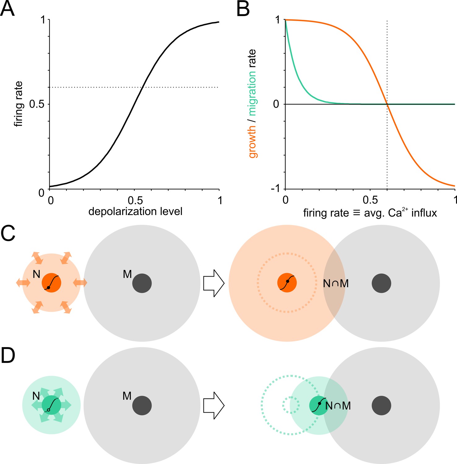
Model of activity-dependent network development.

Neuronal wiring strategies may involve expansion of neurite fields and migration towards other neurons to increase connectivity modeled as neurite field overlap. (A) Transfer function of membrane depolarization between resting and maximal potential to firing rates. *Dotted line*: target firing rate. (B) Neurite growth (orange) and migration (green) were modulated as a function of [Ca²⁺]_i that corresponded to average firing rates. Neurites grew while the firing rate (corresponding to long-term average Ca²⁺ influx) was below target and were pruned when above it. Migration rate decreased as neurons approached the target firing rate (*dotted line*). (C) The area of neurite field overlap, corresponding to connectivity in the model, can be increased by neurite outgrowth and neuronal migration towards neighboring neurons (D).

https://doi.org/10.7554/eLife.47996.002

Figure 2 with 6 supplements

Download asset Open asset

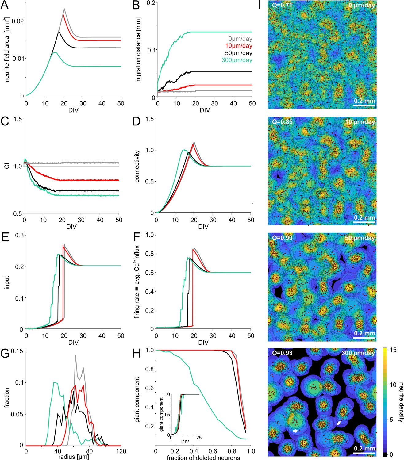
Model of activity-dependent growth and migration.

(A) Activity-dependent growth produced a characteristic overshoot and subsequent pruning of neurite fields. The overall size of developing neurites decreased with increasing migration rates and clustering. (B) Mean migration distance of neurons after seeding (smoothed by 1 hr sliding average). (C) Migration promoted clustering of neurons, which saturated with the onset of network activity and neurite pruning (curves smoothed by 1 hr sliding average). All networks were initialized with the same spatial cell body distribution with CI close to 1. Note that the fluctuations for zero migration results from the random jittering of neuron positions by half the cell body radius (6 µm). (D) Average connectivity increased more rapidly with stronger migration and clustering. (E) Input increased faster with increasing migration rate because clustering initially promoted connectivity. Input levels eventually converged. (F) Firing rates increased sharply once critical input levels were attained. Migration and clustering accelerated the onset of activity. With increasing migration, steps arise because of incremental integration and activation of clusters within the larger network. Note that clustering reduced the developmental overshoot of firing rates. (G) Moderate migration and clustering produced the highest variability of neurite field size across neurons in mature networks. (H) High migration rates increased modularity in mature networks. With increasing migration rate, the giant component more rapidly decreased in clustered networks when a certain fraction of neurons was randomly deleted, indicating that these networks break into disconnected subnets. Inset: the fraction of neurons in the giant cluster, that is the largest connected subnetwork, evolved similarly in different migration conditions. (I) Migration rates crucially determined the mesoscale architecture and modularity (increasing Q indicates stronger modularity) of developing networks. While average neurite fields were small in clustered networks, more isolated neurons generated larger fields (arrows) and formed bottlenecks for activity propagation by connecting otherwise unconnected or weakly connected subnetworks.

https://doi.org/10.7554/eLife.47996.003

Figure 2—figure supplement 1

Download asset Open asset

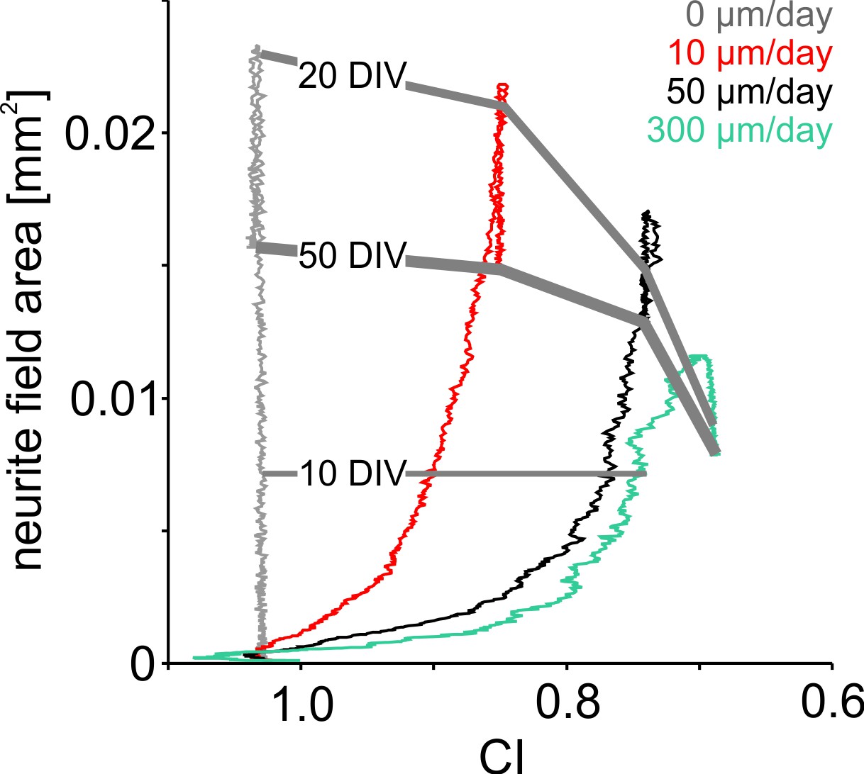
Influence of neuronal clustering on neurite field development.

Increasing migration rates in the simulation promoted neuronal clustering leading to lower final CI and smaller neurite field sizes. At the onset of high network activity, neurite fields were pruned and CI did not change further.

https://doi.org/10.7554/eLife.47996.004

Figure 2—figure supplement 2

Download asset Open asset

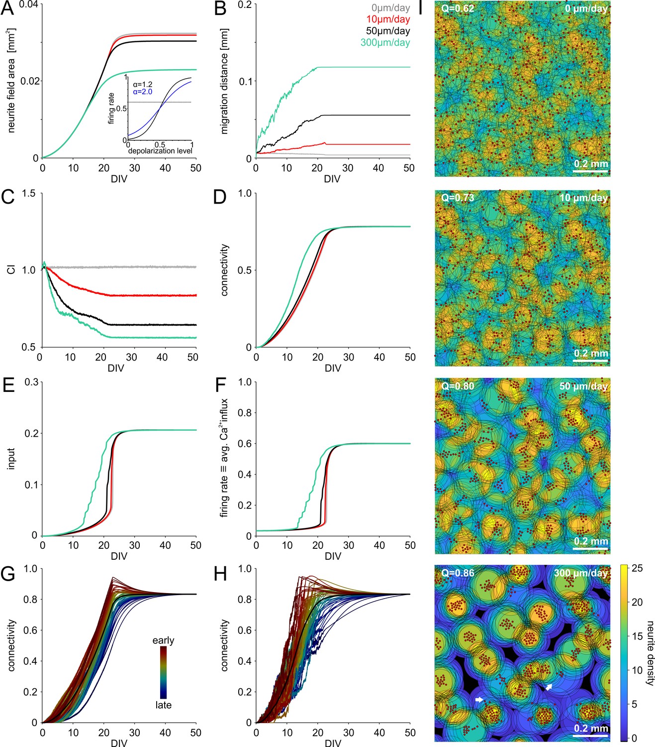
Simulation of saturating network growth.

(A) Decreasing the slope of the sigmoidal transfer function mapping membrane potential to firing rate resulted in saturating growth (inset: blue: $a$ = 0.2) instead of an overshoot (inset: black, $a$ = 0.12, see Figure 2) in average neurite field size and connectivity. Note that the synaptic weight factor $s$ was reduced ( $s$ = 0.05 instead of 0.1) to compensate for the increased baseline firing associated with higher $a$ . Average neurite fields saturated at different levels depending on the rate of migration, average migration distance (B) and degree of clustering (C). (D) Connectivity increased faster with clustering as in the case of $a$ = 0.12. Network-activity, characterized by the average synaptic input (D) and the firing rate (F) increased earlier and more gradually with clustering. (G) Although there was no overshoot of connectivity on average (black line), neurons with faster increase of connectivity showed overshoot and pruning when the network firing rate rapidly increased. In the same network, neurons with slowly increasing connectivity displayed saturating growth. Color indicates the order in which 50 randomly chosen neurons attained 75% of their final connectivity. (H) With migration and clustering, connectivity increased more rapidly with the same dependency of the overshoot on early and late developing connectivity. (I) Saturating growth and migration produced mesoscale network architectures ranging from homogeneous to clustered networks similar to those in Figure 2I. Migration promoted clustering and modularization (increasing Q indicates stronger modularity).

https://doi.org/10.7554/eLife.47996.005

Figure 2—video 1

Download asset

posterframe for video — Simulated network development with migration rate 0 µm/day.
https://doi.org/10.7554/eLife.47996.006

Figure 2—video 2

Download asset

Figure 2—video 3

Download asset

Figure 2—video 4

Download asset

Figure 3 with 2 supplements

Download asset Open asset

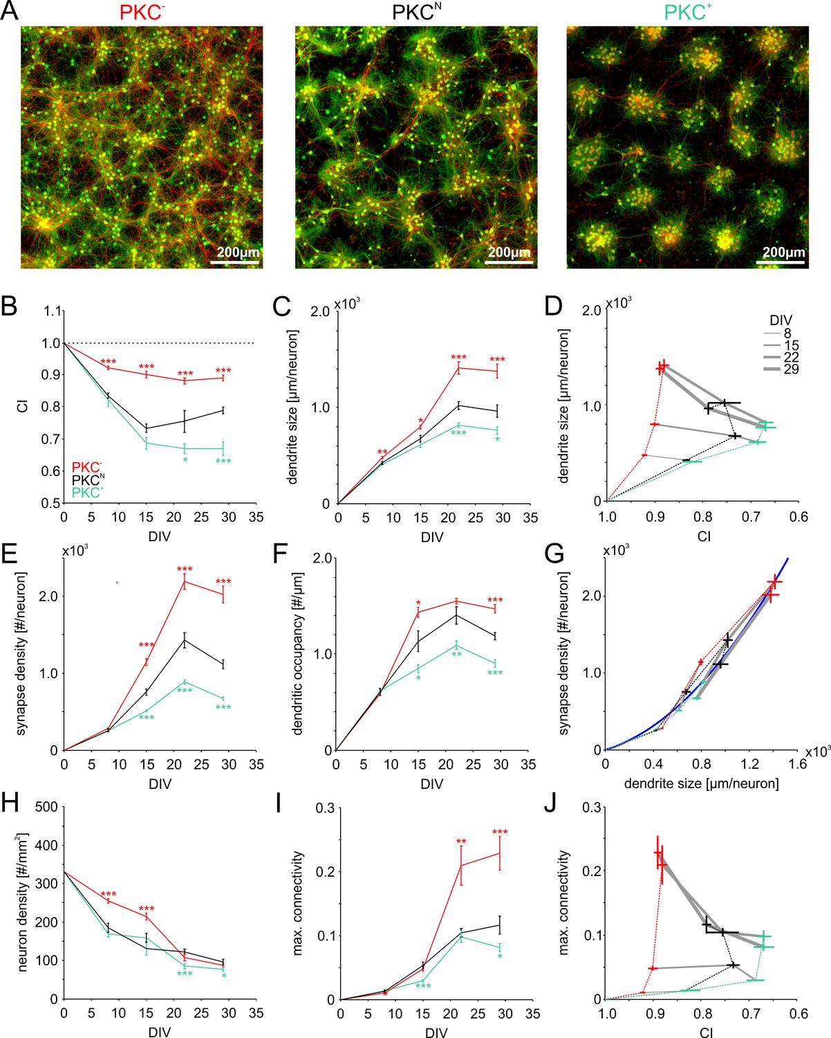
Morphometric analyses of network development.

(A) Dense networks established characteristic mesoscale architectures for the different PKC conditions. PKC⁻ networks had a more homogeneous distribution of axons (red), dendrites (green) and cell bodies (green) than PKC^N networks. In PKC⁺ networks, neurons formed well-delineated clusters. Note that the following morphometric analyses are based on sparser cultures. (B) Decreasing CI during development reflects cell migration and ongoing clustering of neuronal cell bodies until ~15 DIV. PKC⁺ promoted and PKC⁻ diminished clustering during development. (C) Dendrite size increased until 22 DIV, with boosted growth in PKC⁻ and diminished growth in PKC⁺ networks. (D) In late development, dendrite size scaled inversely with the degree of clustering. For visualization the CI axis was inversed, so the degree of clustering increases from left to right. (E) The synapse density increased concurrently with dendrite growth. After 22 DIV synapse densities decreased in PKC^N and PKC⁺ networks, indicating synaptic pruning. (F) Dendritic occupancy with synapses differed slightly between conditions and decreased after 22 DIV. (G) The number of synapse per neurons increased with the dendrite size. Gray lines connect networks of the same age. The blue line illustrates a proposed quadratic scaling rule between dendrite size and synapse densities. (H) Neuron density declined with DIV to about one third of the seeding density. (I) Estimated upper bounds for connectivity based on the synapse density and the total number of neurons (on 113 mm² cover slips). PKC⁻at least doubled average connectivity. (J) In mature networks, maximum connectivity scaled inversely with clustering. All parameters are presented as mean ± SEM. Data from 4 to 24 images (Table 1, area 3.5 mm²) taken in each of 2 networks per condition and age. Asterisks indicate p-values ≤0.05 (*), ≤0.01 (**) and ≤0.001 (***) tested against PKC^N.

https://doi.org/10.7554/eLife.47996.010

Figure 3—source data 1 Source data and Matlab script for Figure 3B,C,E,F,H,I.: https://doi.org/10.7554/eLife.47996.013
Download elife-47996-fig3-data1-v2.zip

Figure 3—figure supplement 1

Download asset Open asset

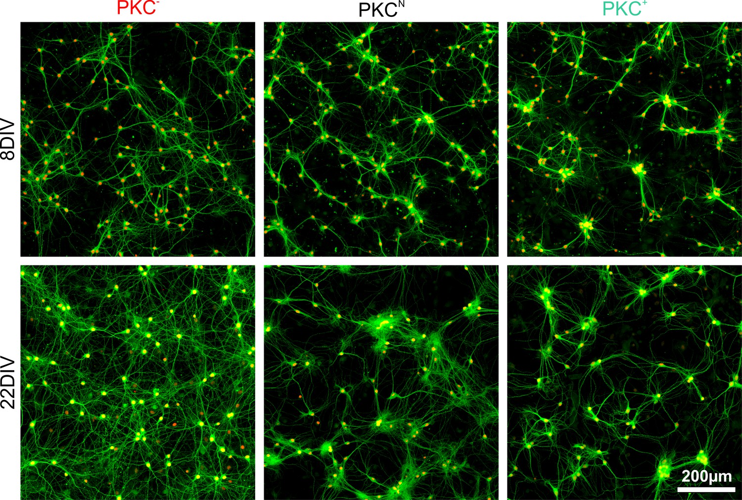
Clustering and dendrite development in sparse networks.

Exemplary images with neuronal nuclei (NeuN, red) and dendrites (MAP2, green) stained at 8 and 22 DIV. PKC inhibition diminished and PKC stimulation promoted neuronal migration and clustering of neurons during development. Dendrite growth changed with the spatial arrangement of cell bodies. Homogeneous cell body arrangements correlated with larger dendrites, whereas clusters had local dendrite tangles and dendrite bundles reaching to other clusters.

https://doi.org/10.7554/eLife.47996.011

Figure 3—figure supplement 2

Download asset Open asset

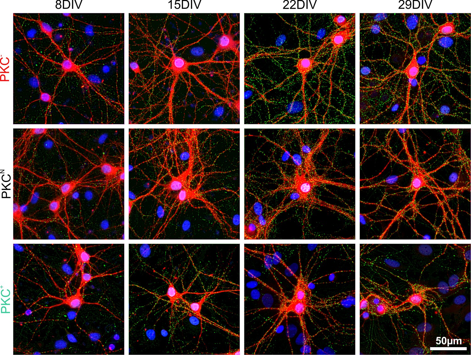
Development of synapses in sparse networks.

Immunohistochemical staining of dendrites (MAP2, red), presynaptic compartments (synapsin, green) and cellular nuclei (DAPI, blue). Synapse densities on dendrites increased in all PKC conditions up to 22 DIV and slightly decreased afterwards. Overall synapse densities were highest in the PKC− and lowest in PKC+ networks.

https://doi.org/10.7554/eLife.47996.012

Figure 4 with 1 supplement

Download asset Open asset

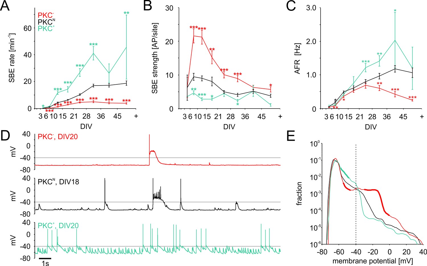
Development of spontaneous network activity.

(A) SBE rates gradually increased during development until 28 DIV, which was accelerated in clustered PKC⁺ networks and decelerated in homogeneous PKC⁻ networks. In result, SBE rates differed considerably in mature networks and increased with the degree of clustering. X-axis ticks indicate bin boundaries. (B) PKC⁻ networks generated stronger SBEs with more APs per site than clustered networks, compensating lower SBE rates to some extent. Burst strength increased initially but declined later on, putatively because of the maturation of inhibition. (C) AFR increased comparably during early development in the different PKC conditions, indicating that stronger bursting compensated lower SBE rates. Later in development, AFRs were increased in PKC⁺ and reduced in PKC⁻ networks. (D) Neurons in PKC⁻ networks showed strong depolarization during SBEs that reached well above the spiking threshold around −40 mV causing depolarization block of spiking. In clustered networks, neurons displayed higher membrane potential fluctuations below threshold that occasionaly passed the threshold leading to spikes. (E) Membrane potential distribution. Thick lines indicate regions significantly different from PKC^N (p≤0.05). The fraction of time in which neuronal membrane potentials were above the spiking threshold (dashed line) was significantly increased in PKC⁻ networks compared to PKC^N and PKC⁺ networks. Data in A-D and F show mean ± SEM derived from 1 hr recording sessions. Asterisks indicate p-values ≤0.05 (*), ≤0.01 (**) and ≤0.001 (***) tested against PKC^N. The number of recordings per age and condition is provided in Table 2.

https://doi.org/10.7554/eLife.47996.017

Figure 4—source data 1 Source data and Matlab script for Figure 4A–C,E.: https://doi.org/10.7554/eLife.47996.019
Download elife-47996-fig4-data1-v2.zip

Figure 4—figure supplement 1

Download asset Open asset

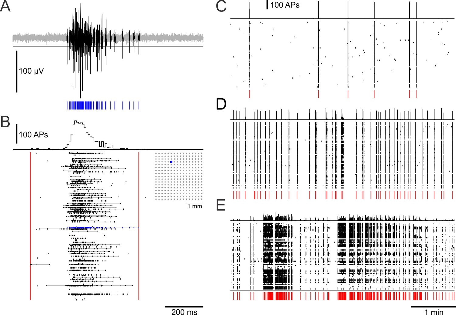
Sample MEA recordings from dense networks.

(A) SBE spike activity on a MEA electrode. Spike times (blue) were detected with a voltage threshold on high-pass filtered raw data. (B) Global spike histogram (10 ms bins) and spike activity of a PKC^N network recorded with a 16 × 16 MEA (inset) at 11 DIV. Most spikes occurred in bursts (gray lines connect spikes assigned to a burst) that were typically organized in SBEs. Red lines indicate SBE onset and offset. Blue: electrode shown in A. (**C–E**) Global spike histogram (top row) and raster plot of typical activity in networks with different mesoscale architecture at 22–23 DIV (58–59 active sites; 6 × 10 MEAs). C SBEs (red ticks) in PKC⁻ networks had high PFRs and typically occurred in regular intervals at low rates. (D) PKC^N networks displayed a wide range of dynamics. The example shows SBEs occuring at intermediate rates and in irregular intervals. (E) Bursts of bursts, that is superbursts, occurred in PKC^N and were very prominent in PKC⁺ (shown), but not in PKC⁻ networks.

https://doi.org/10.7554/eLife.47996.018

Figure 5

Download asset Open asset

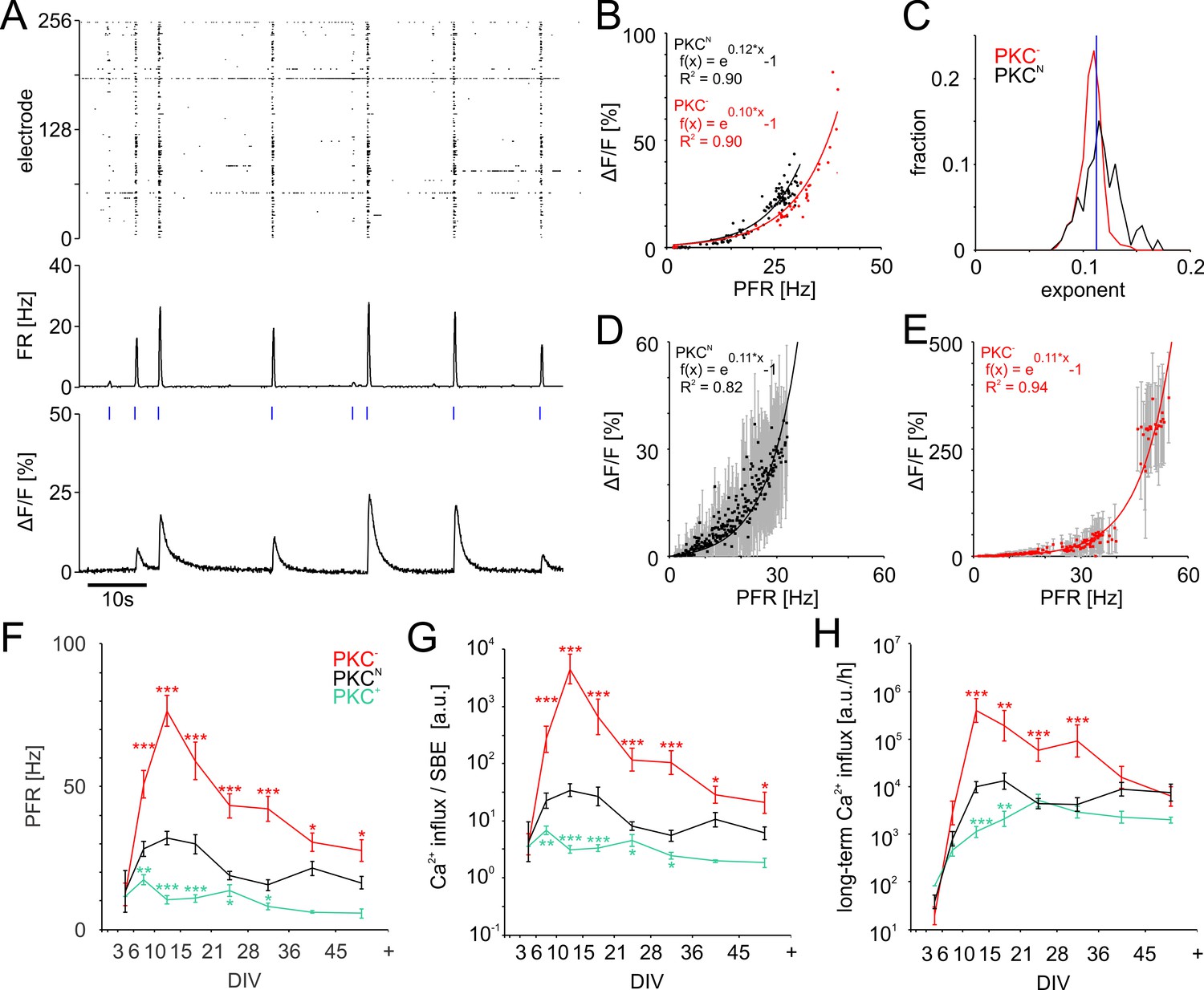
PFR-dependent Ca²⁺ gain.

(A) Spiking raster and firing rate averaged across all electrodes within 40 ms bins (synchronized to the frame times of the Ca²⁺ measurement) and Ca²⁺ signal for one neuronal soma at 19 DIV in a PKC^N network. *Blue ticks*: SBE onsets. (B) The amplitude of Ca²⁺ transients (shown for the PKC^N neuron in A and a PKC⁻ neuron at 20 DIV) scaled exponentially (solid line) with PFR. (C) Exponents had a narrow distribution and were slightly higher in PKC^N (p=3.2*10⁻¹⁸) than in PKC⁻ conditions (PKC^N: 179 neurons, 5 networks at 19 DIV, 714 SBEs total, mean and standard deviation of exponent = 0.12 ± 0.02; PKC⁻: 622 neurons, 4 networks at 20 DIV, 248 SBEs total, exponent = 0.11 ± 0.01). *Blue*: average exponent (0.11 ± 0.01) for the entire data set. (D) Ca²⁺ amplitudes scaled exponentially with PFRs across many neurons in these PKC^N and PKC⁻ networks (E). The data represent median (*data points*) and standard deviation (error bars) of Ca²⁺ amplitudes, averaged across neurons for a given PFR range (bin size 0.1 Hz). (F) PFR assessed during SBEs were higher in homogeneous networks and lower in clustered networks. PFR decreased after week 3, putatively with the maturation of inhibition. (G) Prediction of the development of average Ca²⁺ influx per SBE estimated as $e^{0.11 * P F R} - 1$ (Figure 5D). (H) Average Ca²⁺ influx per minute, estimated from all SBEs in 1 hr recording sessions, suggests that long-term average Ca²⁺ influx in different PKC conditions converged at network maturation. Data in G and H are presented as mean ± SEM. Asterisks indicate p-values ≤0.05 (*), ≤0.01 (**) and ≤0.001 (***) tested against PKC^N.

https://doi.org/10.7554/eLife.47996.021

Figure 5—source data 1 Source data and Matlab script for Figure 5B–E,F.: https://doi.org/10.7554/eLife.47996.022
Download elife-47996-fig5-data1-v2.zip

Figure 6

Download asset Open asset

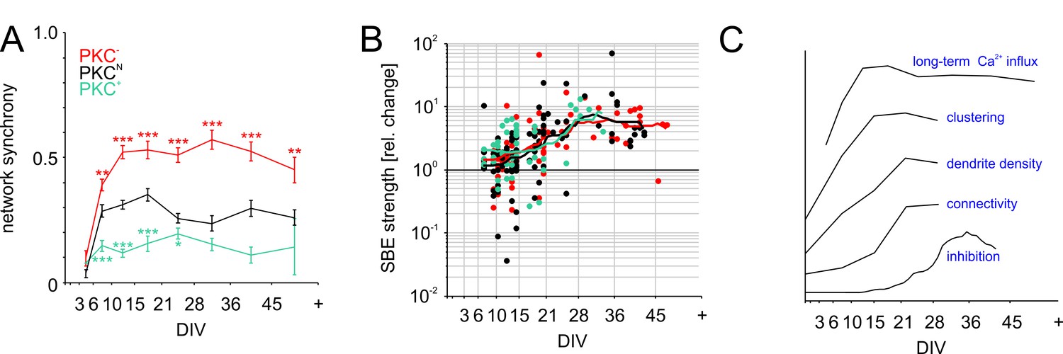
Functional aspects of network maturation.

(A) Network synchrony (average spike train correlation for all electrode pairs determined with 30 ms time bins, mean ± SEM) stabilized early in development in all PKC conditions but was significantly higher in homogeneous networks and significantly lower in clustered networks. Asterisks indicate p-values ≤0.05 (*), ≤0.01 (**) and ≤0.001 (***) tested against PKC^N. (B) Inhibition was probed by acute blockade of GABA-A receptors with PTX. In early networks, PTX had highly variable impact on SBE strength (<14 DIV) but significantly increased it after 21 DIV in all network types. The maturation of inhibition was comparable across PKC conditions. (C) Illustration of the time course of key differentiation processes shown in detail in Figures 3 and 5 in relation to the development of long-term average Ca²⁺ influx. Morphological parameters that showed a similar time course across PKC conditions were normalized to final levels to visualize the relative change during development. The maturation of inhibition is shown as average relative change in SBE strength upon PTX appliction. Y-axis scaling is linear for all graphs. An offset was added for visualization.

https://doi.org/10.7554/eLife.47996.023

Figure 6—source data 1 Source data and Matlab script for Figure 6A,B.: https://doi.org/10.7554/eLife.47996.024
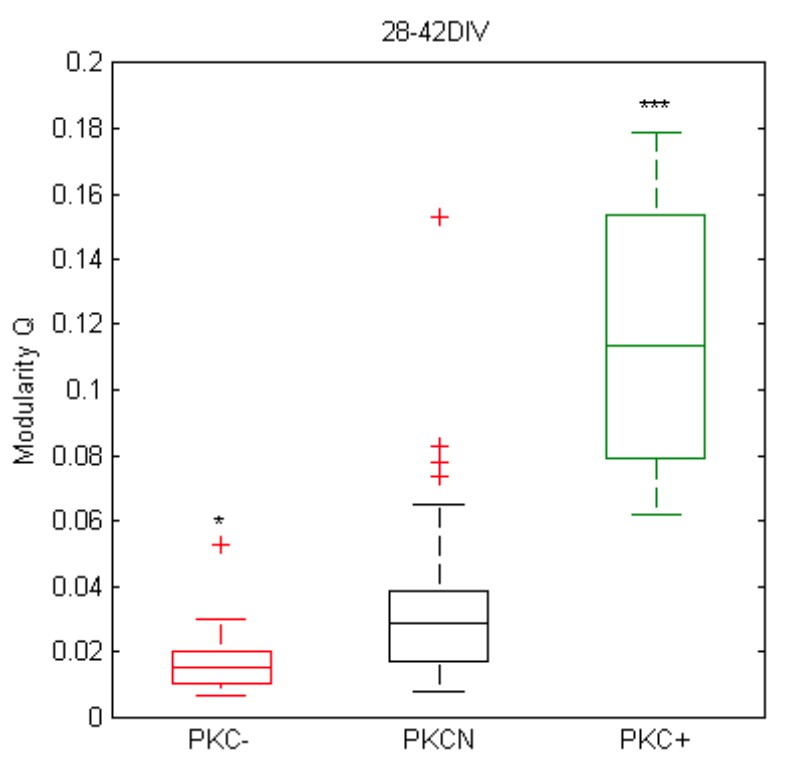
Download elife-47996-fig6-data1-v2.zip

Author response image 1

Download asset Open asset

Tables

Table 1

Morphometric analysis of network development under different PKC conditions.

Results are presented as mean ± standard error of mean (SEM). Significance was determined against PKC^N, or between specified developmental time windows, using independent Student’s t-test. N specifies the number of analyzed images taken from two networks per PKC condition and age.

https://doi.org/10.7554/eLife.47996.014

	DIV	PKC^-	PKC^N	PKC⁺	unit
clustering index
	8	0.92 ± 0.01 (1.8*10⁻¹⁰)	0.84 ± 0.01	0.82 ± 0.02 (6.1*10⁻¹)	CI
	15	0.9 ± 0.01 (1.5*10⁻⁶)	0.73 ± 0.01	0.69 ± 0.02 (1.1*10⁻¹)	CI
	22	0.88 ± 0.01 (4.4*10⁻⁴)	0.75 ± 0.03	0.67 ± 0.02 (3.3*10⁻²)	CI
	29	0.89 ± 0.01 (8.0*10⁻⁹)	0.79 ± 0.01	0.67 ± 0.02 (2.1*10⁻⁵)	CI
	8 vs. 22	−4.49 (3.5*10⁻⁴)	−9.65 (3.1*10⁻²)	−18.6 (1.2*10⁻⁵)	% change
	22 vs. 29	1.04 (4.9*10⁻¹)	4.5 (2.7*10⁻¹)	0.01 (1.0)	% change
Dendrite size
	8	476 ± 9 (1.3*10⁻³)	421 ± 12	408 ± 8 (3.4*10⁻¹)	µm
	15	797 ± 22 (1.2*10⁻²)	676 ± 37	610 ± 30 (2.1*10⁻¹)	µm
	22	1413 ± 64 (7.9*10⁻⁵)	1021 ± 41	816 ± 24 (3.6*10⁻⁴)	µm
	29	1380 ± 74 (1.9*10⁻⁴)	962 ± 65	760 ± 37 (1.3*10⁻²)	µm
	8 vs. 22	196.59 (4.0*10⁻²⁰)	142.46 (9.1*10⁻¹²)	100.08 (1.4*10⁻¹⁵)	% change
	22 vs. 29	−2.38 (7.4*10⁻¹)	−5.81 (5.0*10⁻¹)	−6.86 (2.5*10⁻¹)	% change
Synapse density
	8	281 ± 11 (2.2*10⁻¹)	255 ± 18	254 ± 14 (9.4*10⁻¹)	#
	15	1142 ± 44 (2.3*10⁻⁴)	754 ± 39	510 ± 9 (2.4*10⁻⁵)	#
	22	2188 ± 100 (2.1*10⁻⁵)	1427 ± 99	885 ± 27 (3.4*10⁻⁵)	#
	29	2019 ± 110 (4.5*10⁻⁸)	1114 ± 56	669 ± 21 (5.7*10⁻⁸)	#
	8 vs. 22	678.77 (4.7*10⁻²⁴)	458.69 (2.1*10⁻¹⁰)	248.68 (1.2*10⁻¹⁷)	% change
	22 vs. 29	−7.75 (2.7*10⁻¹)	−21.93 (6.7*10⁻³)	−24.35 (1.2*10⁻⁶)	% change
Dendritic occupancy
	8	0.59 ± 0.02 (6.4*10⁻¹)	0.6 ± 0.04	0.62 ± 0.03 (7.5*10⁻¹)	#/µm
	15	1.44 ± 0.05 (1.7*10⁻²)	1.13 ± 0.11	0.85 ± 0.04 (1.7*10⁻²)	#/µm
	22	1.55 ± 0.03 (9.6*10⁻²)	1.4 ± 0.09	1.09 ± 0.04 (5.7*10⁻³)	#/µm
	29	1.47 ± 0.04 (3.0*10⁻⁵)	1.19 ± 0.04	0.9 ± 0.04 (2.3*10⁻⁵)	#/µm
	8 vs. 22	163.83 (7.2*10⁻²⁸)	132.26 (9.0*10⁻⁸)	76.65 (3.7*10⁻¹⁰)	% change
	22 vs. 29	−5.06 (1.5*10⁻¹)	−15.41 (2.3*10⁻²)	−17.45 (3.8*10⁻³)	% change
Neuron density
	8	255 ± 6 (9.6*10⁻⁷)	185 ± 11	168 ± 7 (2.0*10⁻¹)	#/mm²
	15	214 ± 9 (5.9*10⁻⁴)	131 ± 17	158 ± 12 (2.0*10⁻¹)	#/mm²
	22	107 ± 8 (1.9*10⁻¹)	123 ± 6	85 ± 6 (5.7*10⁻⁴)	#/mm²
	29	87 ± 5 (3.0*10⁻¹)	96 ± 7	77 ± 4 (2.6*10⁻²)	#/mm²
	8 vs. 22	−58.03 (7.3*10⁻¹⁷)	−33.66 (1.1*10⁻⁴)	−49.42 (1.0*10⁻⁸)	% change
	22 vs. 29	−18.93 (4.5*10⁻²)	−21.71 (1.3*10⁻²)	−9.79 (2.6*10⁻¹)	% change
Maximum connectivity
	8	0.01 ± 0.001 (3.5*10⁻²)	0.013 ± 0.001	0.014 ± 0.001 (6.3*10⁻¹)	fraction
	15	0.048 ± 0.003 (4.6*10⁻¹)	0.053 ± 0.006	0.029 ± 0.002 (9.2*10⁻⁴)	fraction
	22	0.209 ± 0.031 (8.2*10⁻³)	0.104 ± 0.007	0.098 ± 0.009 (5.9*10⁻¹)	fraction
	29	0.229 ± 0.026 (9.2*10⁻⁴)	0.116 ± 0.014	0.081 ± 0.006 (3.8*10⁻²)	fraction
	8 vs. 22	1987.43 (5.9*10⁻¹⁰)	701.18 (2.6*10⁻¹¹)	604.32 (1.4*10⁻¹⁰)	% change
	22 vs. 29	9.31 (6.3*10⁻¹)	11.48 (5.2*10⁻¹)	−17.23 (1.3*10⁻¹)	% change
N
	8	24	11	15
	15	9	4	7
	22	15	11	11
	29	17	16	15

Table 1—source data 1 Source data and Matlab script.: https://doi.org/10.7554/eLife.47996.015
Download elife-47996-table1-data1-v2.zip
Table 1—source data 2 Source data and Matlab script.: https://doi.org/10.7554/eLife.47996.016
Download elife-47996-table1-data2-v2.zip

Table 2

Electrophysiological characterization of network activity during development.

Data were pooled within defined developmental time windows. Significance was determined against PKC^N using independent Student’s t-test. N specifies the number of recorded networks per PKC condition and age.

https://doi.org/10.7554/eLife.47996.020

	DIV	PKC⁻	PKC^N	PKC⁺
AFR
	3–5	0.03 ± 0.01 (1.0*10⁻¹)	0.05 ± 0.01	0.09 (1.4*10⁻¹)
	6–9	0.08 ± 0.01 (2.6*10⁻³)	0.18 ± 0.03	0.1 ± 0.02 (4.0*10⁻²)
	10–14	0.36 ± 0.04 (1.8*10⁻²)	0.49 ± 0.03	0.42 ± 0.04 (2.0*10⁻¹)
	15–20	0.53 ± 0.06 (3.6*10⁻¹)	0.61 ± 0.06	0.76 ± 0.19 (3.6*10⁻¹)
	21–27	0.69 ± 0.08 (2.5*10-¹)	0.8 ± 0.06	1.21 ± 0.12 (7.3*10⁻⁴)
	28–35	0.6 ± 0.07 (2.9*10⁻³)	0.96 ± 0.09	1.41 ± 0.15 (6.9*10⁻³)
	36–44	0.42 ± 0.08 (2.4*10⁻⁷)	1.18 ± 0.1	2.04 ± 0.83 (4.3*10⁻²)
	45+	0.24 ± 0.02 (9.9*10⁻⁸)	1.06 ± 0.14	1.2 ± 0.63 (8.3*10⁻¹)
SBE rate (SBE/min)
	3–5	0.17 ± 0.04 (2.9*10⁻¹)	0.11 ± 0.03	0.54 (1.5*10⁻²)
	6–9	0.18 ± 0.03 (5.4*10⁻⁶)	1.02 ± 0.15	1.46 ± 0.19 (7.4*10⁻²)
	10–14	1.21 ± 0.13 (2.0*10⁻⁸)	4.26 ± 0.44	11.69 ± 1.27 (3.4*10⁻¹⁰)
	15–20	2.83 ± 0.35 (1.4*10⁻⁸)	6.36 ± 0.43	14.31 ± 2.03 (4.7*10⁻⁷)
	21–27	4.58 ± 0.44 (2.4*10⁻¹⁰)	10.3 ± 0.62	26.82 ± 3 (5.5*10⁻¹²)
	28–35	4.98 ± 0.81 (2.2*10⁻¹³)	16.97 ± 1.07	41.1 ± 5.07 (7.9*10-⁹)
	36–44	4.08 ± 0.75 (9.0*10⁻¹²)	17.25 ± 1.28	26.21 ± 7.05 (8.7*10⁻²)
	45+	3.74 ± 0.56 (2.2*10⁻¹³)	18.85 ± 1.62	45.76 ± 23.86 (2.0*10⁻³)
SBE strength (APs per burst)
	3–5	6.2 ± 3 (1.0*10⁰)	6.2 ± 3.8	3.5 (7.6*10⁻¹)
	6–9	21.6 ± 2.1 (9.4*10⁻⁷)	9.5 ± 1	4.6 ± 0.6 (1.2*10⁻³)
	10–14	21.2 ± 2.1 (5.7*10⁻⁹)	9 ± 0.8	2.7 ± 0.5 (1.5*10⁻⁷)
	15–20	15.2 ± 1.9 (2.1*10⁻³)	8 ± 1.3	2.7 ± 0.3 (1.2*10⁻²)
	21–27	10.1 ± 1 (6.1*10⁻⁸)	4.9 ± 0.4	4.4 ± 0.9 (5.4*10⁻¹)
	28–35	8.9 ± 0.9 (2.9*10⁻⁶)	4 ± 0.5	2.3 ± 0.3 (1.7*10⁻²)
	36–44	6.2 ± 0.6 (2.2*10⁻¹)	5.1 ± 0.6	5.1 ± 1.6 (9.8*10⁻¹)
	45+	5.6 ± 0.8 (4.2*10⁻²)	3.8 ± 0.5	1.1 ± 0.4 (2.2*10⁻¹)
PFR (Hz)
	3–5	12.3 ± 3.8 (9.0*10⁻¹)	13.2 ± 7.3	11.5 (9.2*10⁻¹)
	6–9	50.8 ± 4.8 (6.4*10⁻⁵)	28.3 ± 2.7	17.4 ± 1.7 (4.9*10⁻³)
	10–14	76.6 ± 5.4 (6.7*10⁻¹⁴)	32.1 ± 2.3	10.3 ± 1.4 (2.1*10⁻⁹)
	15–20	59.1 ± 6.5 (5.3*10⁻⁵)	29.8 ± 3.4	10.9 ± 1.3 (6.4*10⁻⁴)
	21–27	43.3 ± 4.1 (7.4*10⁻¹⁰)	18.9 ± 1.5	13.7 ± 2 (4.4*10⁻²)
	28–35	42.3 ± 4.4 (2.4*10⁻⁸)	15.5 ± 2	8.1 ± 1.2 (1.8*10⁻²)
	36–44	30.5 ± 3.1 (2.7*10⁻²)	21.4 ± 2.6	6.1 ± 0.4 (1.3*10⁻¹)
	45+	27.5 ± 3.8 (1.5*10⁻²)	16.4 ± 2.3	5.6 ± 1.7 (2.8*10⁻¹)
Network synchrony
	3–5	0.1 ± 0.03 (2.6*10⁻¹)	0.04 ± 0.02	0.08 (3.4*10⁻¹)
	6–9	0.39 ± 0.02 (3.3*10⁻³)	0.29 ± 0.02	0.15 ± 0.02 (3.1*10⁻⁴)
	10–14	0.52 ± 0.03 (2.5*10⁻¹⁰)	0.31 ± 0.02	0.12 ± 0.02 (1.4*10⁻¹⁰)
	15–20	0.53 ± 0.04 (4.6*10⁻⁵)	0.35 ± 0.02	0.16 ± 0.03 (1.7*10⁻⁵)
	21–27	0.51 ± 0.03 (5.8*10⁻¹³)	0.26 ± 0.02	0.2 ± 0.02 (4.8*10⁻²)
	28–35	0.57 ± 0.04 (2.0*10⁻¹⁰)	0.24 ± 0.03	0.15 ± 0.03 (7.6*10⁻²)
	36–44	0.53 ± 0.04 (1.3*10⁻⁵)	0.3 ± 0.03	0.11 ± 0.03 (1.3*10⁻¹)
	45+	0.45 ± 0.05 (2.5*10⁻³)	0.26 ± 0.03	0.14 ± 0.11 (3.8*10⁻¹)
N
	3–5	7	3	1
	6–9	33	40	24
	10–14	70	92	47
	15–20	53	65	27
	21–27	77	121	56
	28–35	47	62	29
	36–44	38	57	4
	45+	38	36	2

Key resources table

Reagent type (species) or resource	Designation	Source or reference	Identifiers	Additional information
Strain, strain background (Rattus norvegicus domestica)	wildtype wistar rat pups	CEMT, University, Freiburg
Genetic reagent	AAV9.CAG.GCaMP6s.WPRE.SV40	Penn Vector Core, University of Pennsylvania	V3296TI-R	titer 1e11
Antibody	anti-MAP2 (chicken polyclonal)	Abcam, Cambridge, UK	ab92434 RRID:AB_2138147	1:500
Antibody	anti-NeuN (rabbit polyclonal)	Abcam, Cambridge, UK	ab128886 RRID:AB_2744676	1:500
Antibody	anti-Neurofilament (mouse monoclonal)	Abcam, Cambridge, UK	ab24571 RRID:AB_448148	1:10
Antibody	anti-Synapsin (mouse monoclonal)	Synaptic Systems GmbH, Germany	106001 RRID:AB_887805	1:200
Antibody	anti-chicken-Cy2 (goat polyclonal)	Abcam, Cambridge, UK	ab6960 RRID:AB_955003	1:200
Antibody	anti-rabbit-Cy3 (goat polyclonal)	Abcam, Cambridge, UK	ab6939 RRID:AB_955021	1:200
Antibody	anti-mouse-Cy5 (goat polyclonal)	Abcam, Cambridge, UK	ab6563 RRID:AB_955068	1:200
Chemical compound, drug	4,6-diamidino-2-phenyindole, diclactate (DAPI)	Sigma-Aldrich, Germany	D9562	1:5000
Chemical compound, drug	Gödecke6976	Tocris Bioscience, Bristol, UK	2253	1 µM
Chemical compound, drug	Phorbol-12-Myristate-13-Acetate (PMA)	Sigma-Aldrich, Munich, Germany	P1585	1 µM
Chemical compound, drug	Picrotoxin	Tocris Bioscience, Bristol, UK	1128	10 µM
Chemical compound, drug	DMSO	Sigma-Aldrich, Munich, Germany	D8418	0.1%
Chemical compound, drug	DNase (type IV)	Sigma-Aldrich, Munich, Germany	D5025	50 g/ml
Chemical compound, drug	minimal essential medium	Invitrogen, Karlsruhe, Germany	21090055
Chemical compound, drug	horse serum (heat-inactivated)	Invitrogen, Karlsruhe, Germany	26050088	20%
Chemical compound, drug	phosphate buffered saline (PBS)	Invitrogen, Karlsruhe, Germany	21600010
Chemical compound, drug	glucose	Sigma-Aldrich, Munich, Germany	G7528	20 mM
Chemical compound, drug	L-glutamine	Invitrogen, Karlsruhe, Germany	25030024	0.5 mM
Chemical compound, drug	gentamycin	Invitrogen, Karlsruhe, Germany	15750060	20 µg/ml
Chemical compound, drug	potassiumD-gluconate	Sigma-Aldrich, Munich, Germany	G4500	125 mM
Chemical compound, drug	EGTA	Carl Roth, Karlsruhe, Germany	3054	5 mM
Chemical compound, drug	KCl	Sigma-Aldrich, Munich, Germany	P4504	20 mM
Chemical compound, drug	Na₂-ATP	Carl Roth, Karlsruhe, Germany	K054	2 mM
Chemical compound, drug	Hepes	Carl Roth, Karlsruhe, Germany	9105	10 mM
Chemical compound, drug	CaCl₂	Sigma-Aldrich, Munich, Germany	C3881	0.5 mM
Chemical compound, drug	KOH	Sigma-Aldrich, Munich, Germany	P4504
Chemical compound, drug	MgCl₂	Sigma-Aldrich, Munich, Germany	MO250	2 mM
Software	MC Rack software	Multi Channel Systems, Germany	versions 3.3–4.5 RRID:SCR_014955
Software	Spike2 software	Cambridge Electronics Design Ltd., Cambridge, UK.	RRID:SCR_000903
Software	Zen	Carl Zeiss, Jena, Germany	RRID:SCR_013672
Software	MEA-Tools	Egert et al., 2002 (PMID 12084562)	version 2.8
Software	FIND toolbox	Meier et al., 2008 (PMID 18692360)
Software	ImageJ	Schneider et al., 2012 (PMID 22930834)	RRID:SCR_003070
Software	Matlab	Mathworks, Natick, MA, USA	versions 2014a – 2017a