High-throughput microcircuit analysis of individual human brains through next-generation multineuron patch-clamp
- Charité – Universitätsmedizin Berlin, Germany
Figures
Figure 1

Multipatch setups.
(A) Overview of essential components of a 10-manipulator setup with Sensapex micromanipulators. (B) Side view depicting the spatial arrangement of a manipulator including headstage and pipette relative to the recording chamber which is elevated above the condensor. The dashed outline shows the manipulator with pipette tip immersed in the cleaning solution. (C) Top view of 10 Sensapex manipulators with headstages and their angles to each other on the custom-made stage. (D) Top view of 8 Scientifica PatchStar manipulators with headstages and their angles to each other on a custom-made ring-shaped stage. (E) Photograph of the 10-manipulator setup. (F) Photograph of the eight-manipulator setup.
Figure 2 with 1 supplement
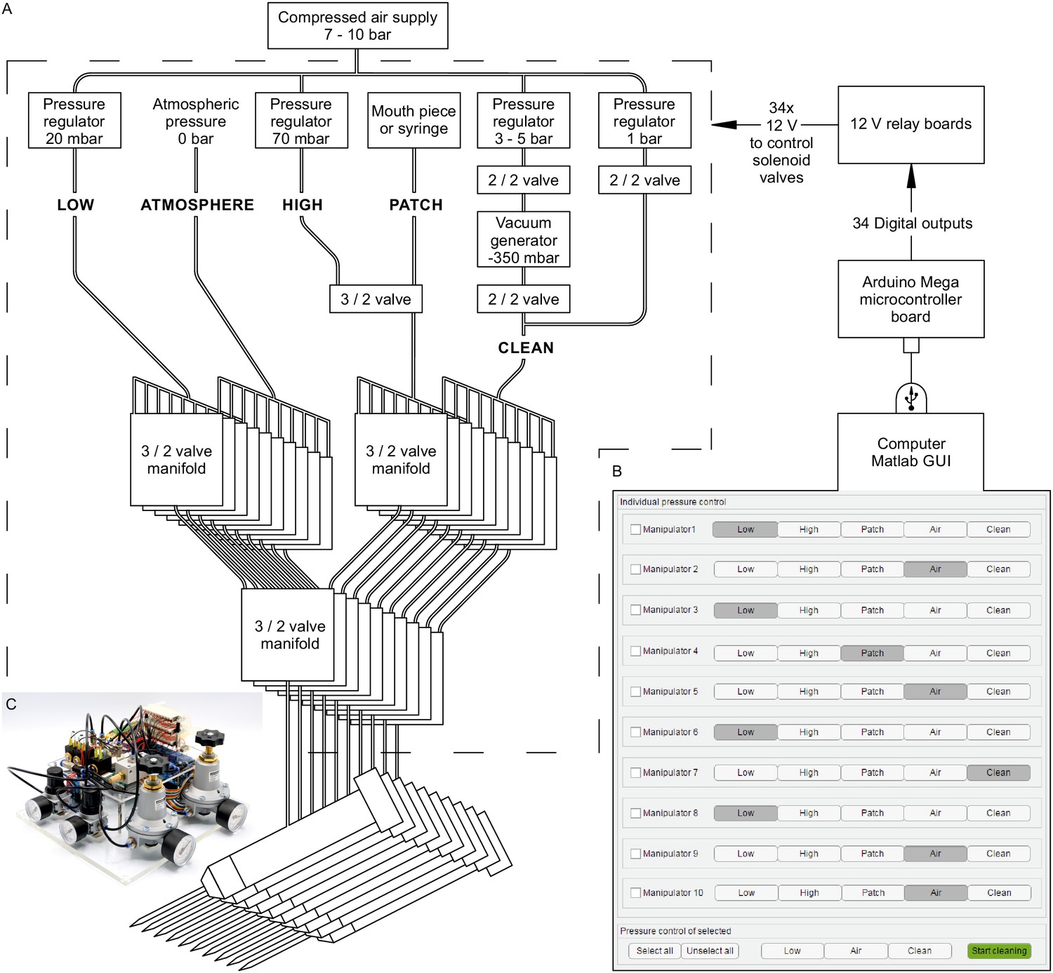
Automated pressure system.
(A) Tubing scheme between the different pneumatic components. Top row depicts pressure regulators and their set pressure for each path. 2/2 valves are solenoid valves with two ports and two positions (open or closed). 3/2 valves are miniature solenoid valves with three ports and can switch between two positions connecting either inlet to one outlet. An illustrated step-by-step assembly guide of the pressure system can be found in Appendix 1. (B) Screenshot of Matlab GUI controlling the pressure system. It communicates with an Arduino microcontroller board which in turn has digital outputs connecting onto a relay board. For further details of wiring scheme see Figure 2—figure supplement 1. For more information on GUI see appendix 2. (C) Photograph of an assembled pressure system.
Figure 2—figure supplement 1
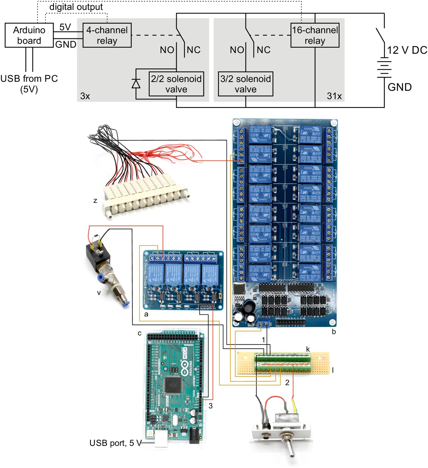
Wiring scheme of pressure system.
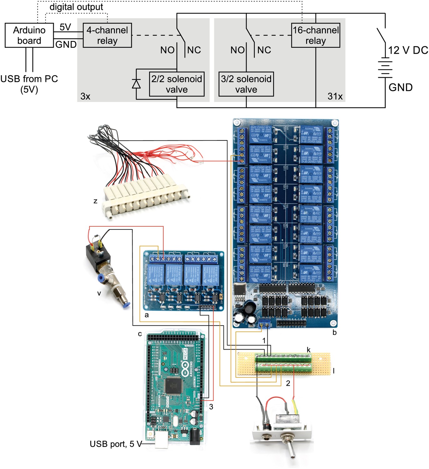
Top: Electrical circuit wiring diagram for valves, relays and Arduino board. This wiring diagram shows that all solenoid valves (z, v) and the two 16-channel relay board (b) are powered through the 12 V DC power supply (80 W, 12 V / 6,67 A). The four-channel relay is powered through the Arduino board which receives a 5 V power supply from the USB cable. The gray boxes indicate that this circuit is replicated for each valve in parallel. The relays receive digital signals from the Arduino boards (dotted lines) and switch the contacts from NC (normally closed) to NO (normally open) which brings the solenoid valve into a different state. A flyback diode is necessary for the 2/2 solenoid valves to protect from voltage spikes. Bottom: Photographic wiring scheme of circuit. (1) Ground conductor is connected to all black lines through the soldered screw block on the stripboard (k, l). (2) The 12 V phase conductor (red) is connected to all yellow lines through the other soldered screw terminal block. These yellow wires carry 12 V to power the 16-channel relay board (b), the individual 3/2 solenoid valves (z) and the 2/2 solenoid valves (v). (3) The 4-channel relay board (a) is powered through the 5 V output pin of the Arduino board (c) which is supplied through the USB-cable from the PC.
Figure 3 with 5 supplements
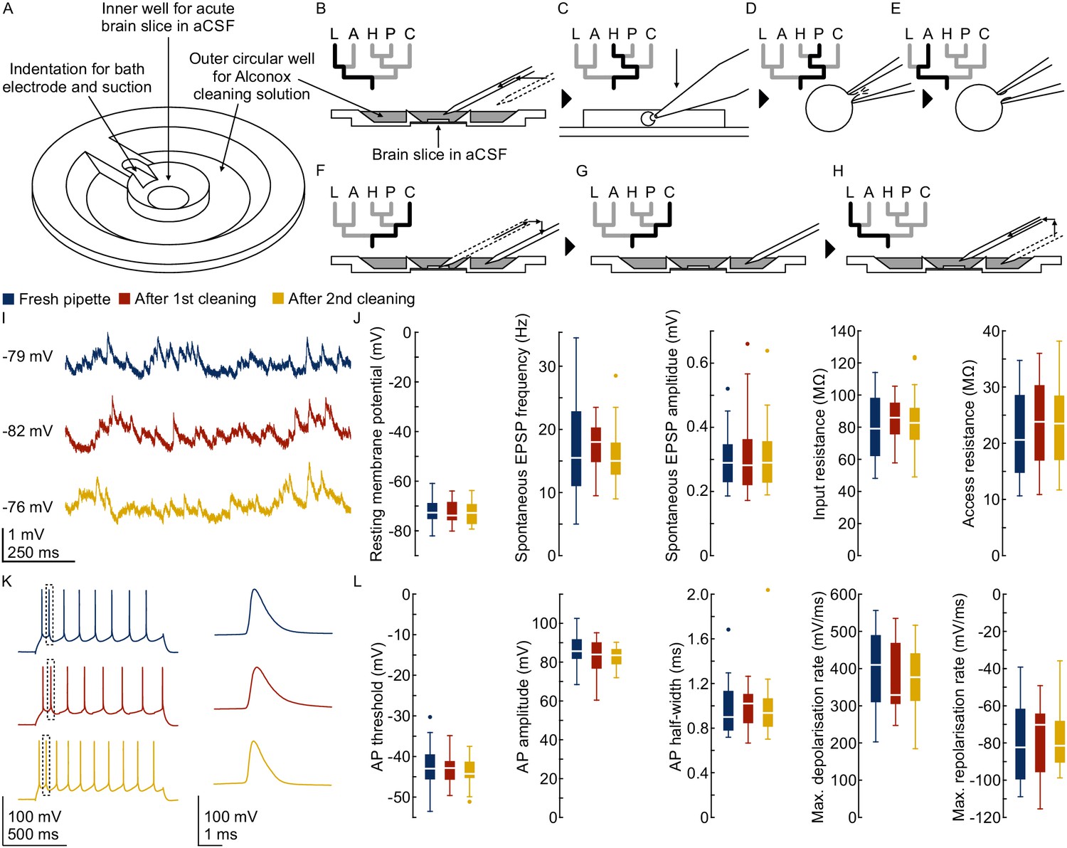
Pipette cleaning protocol.
(A) Design of custom-made recording chamber with one centre well for the brain slice and recording solution and another circular outer well for the cleaning solution, see construction design in Appendix 1—figure 1 and 2. (B–H) Experimental steps for pipette cleaning. Tree diagrams on the top left depict the configuration of the pressure system with the following pressure levels: LOW, ATMOSPHERE, HIGH, PATCH, CLEAN. (B) Pipettes are moved into the recording solution with LOW pressure. (C) Cells are approached with HIGH pressure. (D) Formation of gigaseal and membrane rupture with pressures applied through the PATCH channel with either mouth piece or syringe. (E) Cells are kept at ATMOSPHERE pressure after successful patch. (F) Pipettes are moved into the cleaning solution and switched to CLEAN pressure. (G) Cleaning pressure sequence is applied in the outer well. (H) Pipettes are moved back into the recording solution above the slice and switched to LOW pressure. (I) Current clamp traces at resting membrane potential exhibiting spontaneous EPSPs recorded using the same pipette before (blue) and after cleaning (red and yellow). (J) Box plots of cellular, synaptic and recording properties of cells recorded with fresh (blue, n = 25, except n = 23 for synaptic parameters) and cleaned pipettes (red, n = 21 and yellow, n = 21). (K) Action potential firing patterns elicited through step current injection and enlarged action potential traces recorded on the same pipette before (blue) and after cleaning (red and yellow). (L) Box plots of action potential properties of cells recorded with fresh (blue, n = 25) and cleaned pipettes (red and yellow, n = 21). Further statistical information and analysis are shown in Figure 3—source data 1.
-
Figure 3—source data 1
Statistical summary intrinsic parameters.
- https://cdn.elifesciences.org/articles/48178/elife-48178-fig3-data1-v2.xlsx
-
Figure 3—source data 2
Statistical summary synaptic parameters.
- https://cdn.elifesciences.org/articles/48178/elife-48178-fig3-data2-v2.xlsx
Figure 3—figure supplement 1

Fresh pipette vs. cleaned pipette.
Boxplots depict the intrinsic electrophysiological properties of different human neurons patched either with fresh pipettes (blue, n = 24) or cleaned pipettes (red, n = 9). Further statistical data in Figure 3—source data 1.
Figure 3—figure supplement 2
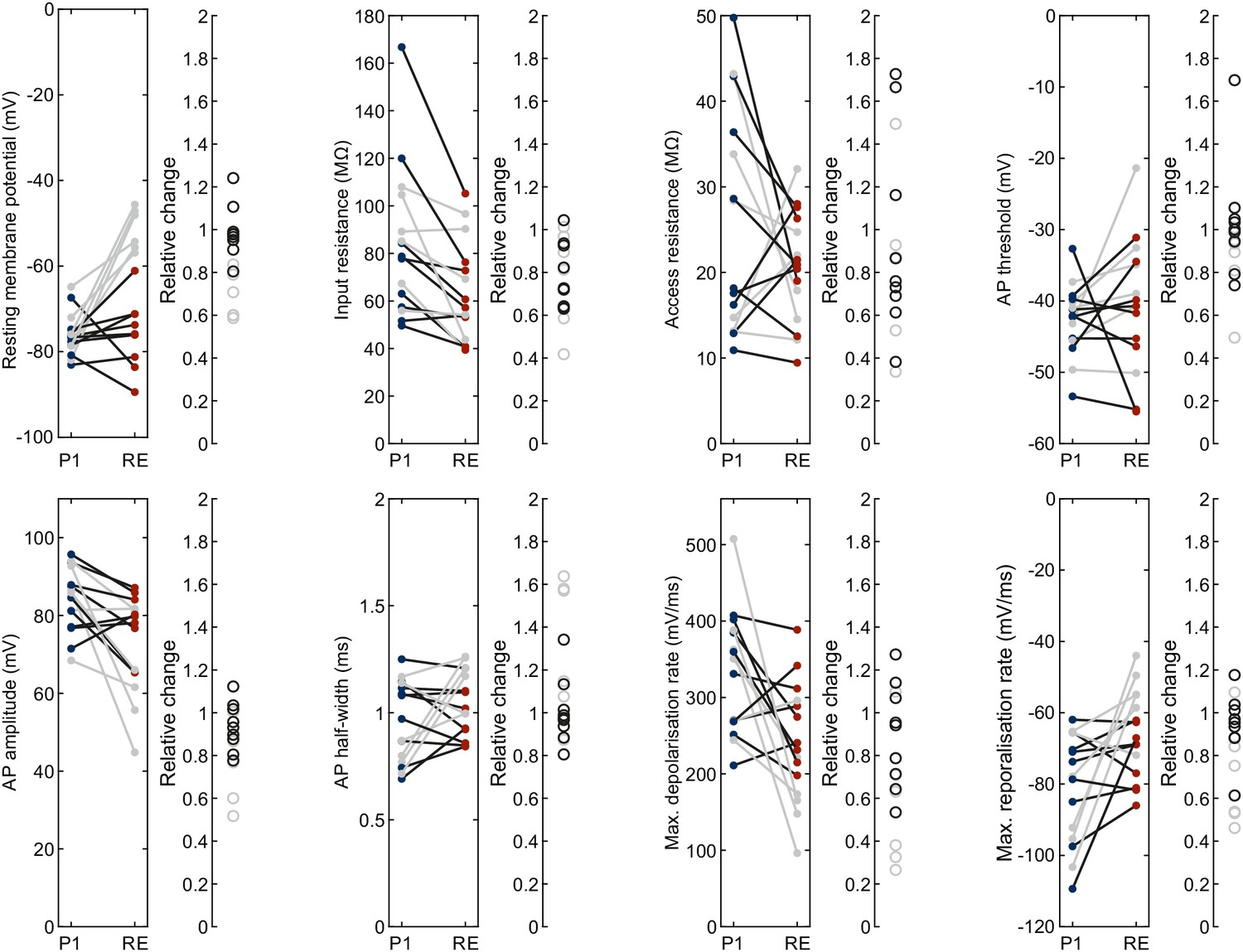
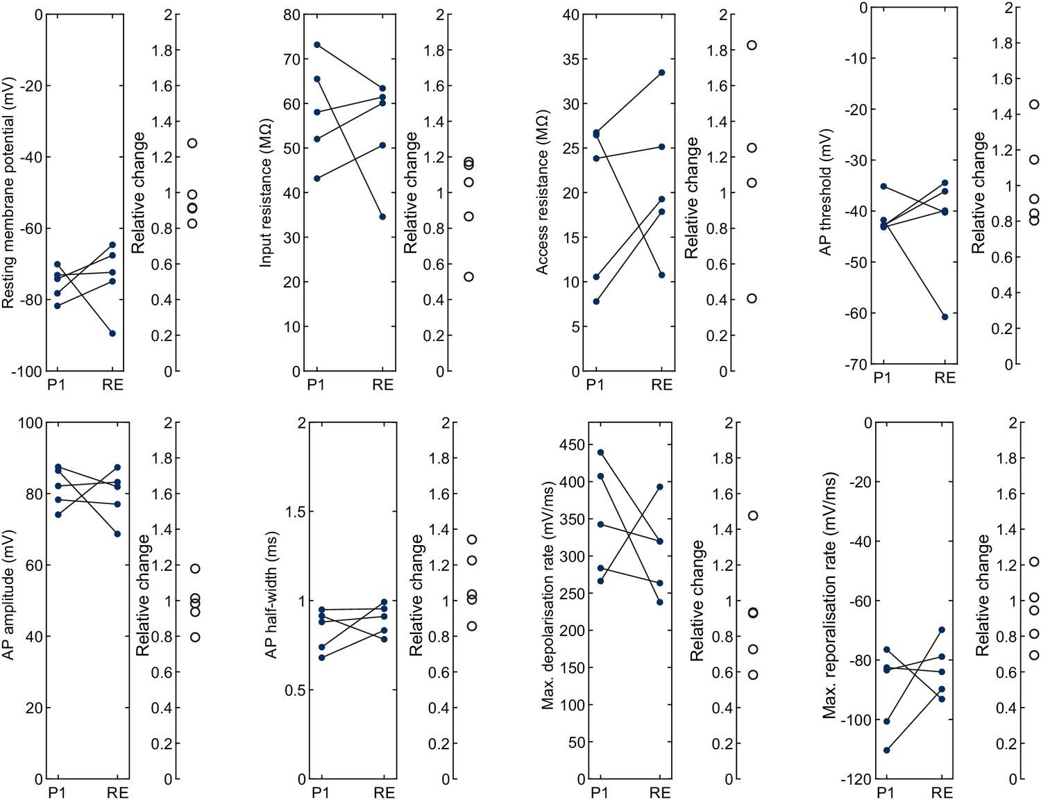
Fresh pipette vs. repatch of same cell with cleaned pipette.
Left panel with line plots shows the intrinsic electrophysiological properties of the same human neuron (each line) patched with a fresh pipette (‘P1’, blue) and repatched with the same pipette after cleaning (‘RE’, red). Right panel shows the relative change for each neuron. Out of 15 neurons, 9 were included (black lines and circles) and 6 were excluded due to depolarised resting membrane potential after repatch (gray lines and circles). Further statistical data in Figure 3—source data 1.
Figure 3—figure supplement 3
Fresh pipette vs. repatch with fresh pipette.
Left panel with line plots shows the intrinsic electrophysiological properties of the same human neuron (n = 5, each line) patched with a fresh pipette (‘P1’, blue) and repatched with another fresh pipette (‘RE’, blue). Right panel shows the relative change for each neuron. Further statistical data in Figure 3—source data 1.
Figure 3—figure supplement 4
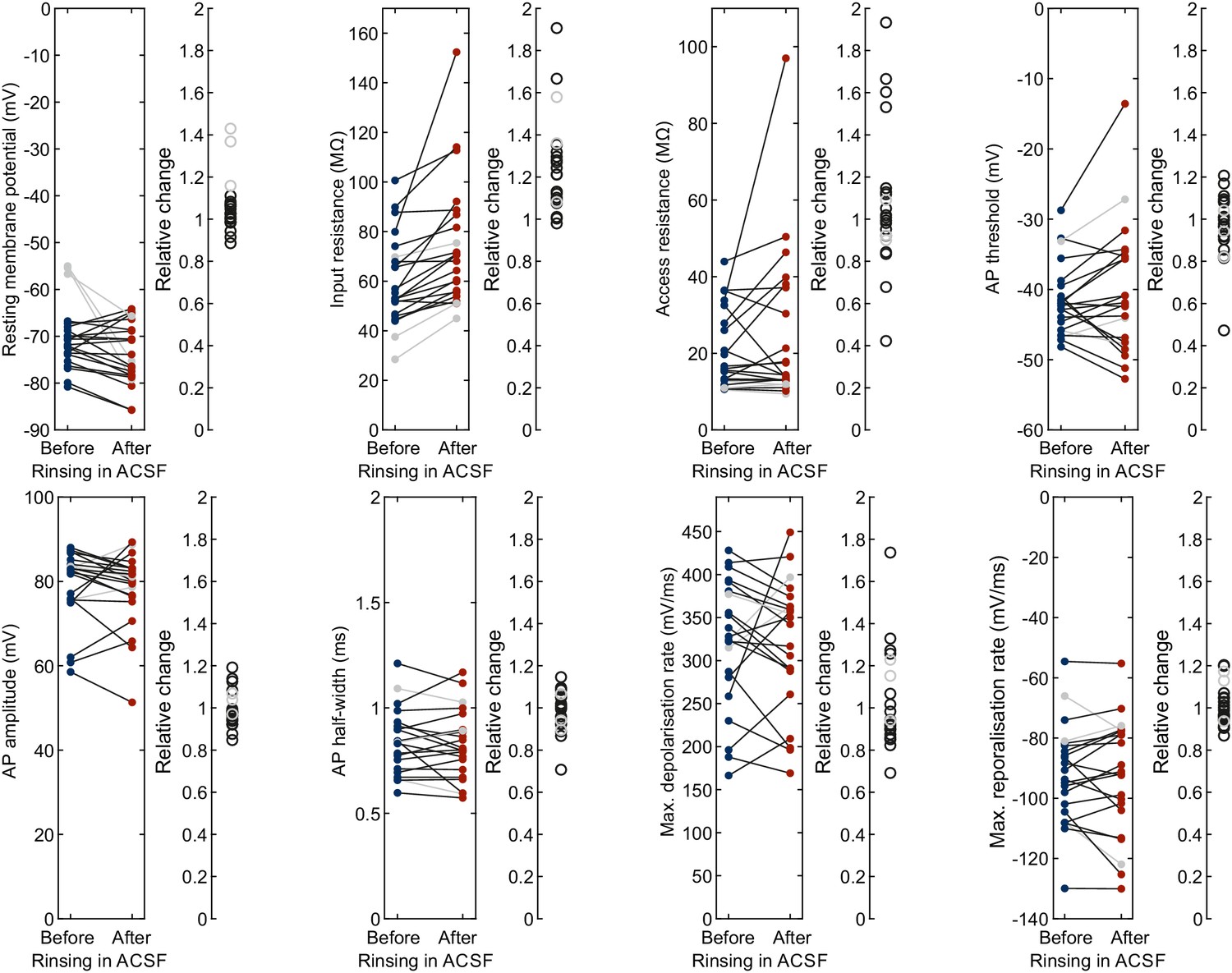
ACSF before vs. after rinsing during cleaning.
Left panel with line plots shows the intrinsic electrophysiological properties of the same human neuron (each line) patched with a fresh pipette in fresh ACSF (‘Before’, blue) and consecutively held in ACSF which has been subject to rinsing during the cleaning of two other pipettes (‘After’, red). Right panel shows the relative change for each neuron. Out of 22 neurons, 19 were included (black lines and circles) and three were excluded due to depolarised resting membrane potential in the initial recording (gray lines and circles). Further statistical data in Figure 3—source data 1.
Figure 3—figure supplement 5

Synaptic amplitudes recorded in ACSF before vs. after rinsing during cleaning.
Boxplots show distribution of individual excitatory postsynaptic potential amplitudes acquired from connected human neuronal pairs (n = 20 individual sweeps). Seven synaptic pairs were recorded in fresh ACSF (blue) and again recorded in ACSF which has been subject to rinsing during the cleaning of other pipettes (red). Synaptic pair two showed a significant increase, while synaptic pair three showed a significant decrease in amplitude (Mann-Whitney U Test). Overall, neither a significant trend toward increasing or decreasing amplitudes were found. Further statistical data in Figure 3—source data 2.
Figure 4
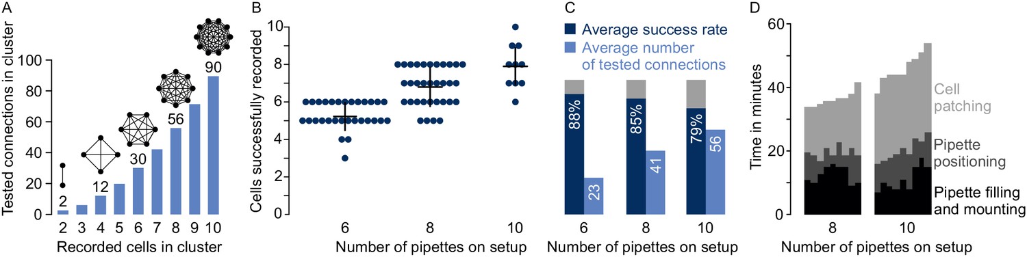
Performances on multipatch setups.
(A) Bar graphs depicting maximum number of testable connections for increasing number of simultaneously recorded cells. (B) Dot plot of number of simultaneously recorded cells from rodent brain slice experiments using different multipatch setups. Black crosses indicate mean and standard deviation. (C) Performance parameters derived from B. Average success rate represents the average size of recorded clusters in relation to the maximally possible cell number given the available pipettes on each setup. Average numbers of tested connections are derived from the number of tested connections from each experiment. Note the decrease in success rate and slowing increase of tested connections when the number of pipettes is increased. (D) Stacked bar graph of time needed for individual preparatory steps of single experiments for the eight-manipulator setup (n = 9) and the 10-manipulator setup (n = 9). Source data provided in Figure 4—source data 1 and Figure 5—source data 1.
-
Figure 4—source data 1
Source Data - experimental times.
- https://cdn.elifesciences.org/articles/48178/elife-48178-fig4-data1-v2.xlsx
Figure 5 with 1 supplement

Different strategies for cleaning pipettes.
(A) Scheme of successful whole-cell recordings on six pipettes (blue circles with action potentials) and failed patch attempts on two pipettes (white circles without action potentials). (B) Clean-to-complete: The two failed pipettes were cleaned and successful recordings were established from two neighbouring cells. Red circles represent a cluster that has been subject to pipette cleaning after failed patch attempts and the red lines indicate the tested synaptic connections. (C) Dot plot comparing the number of successfully recorded neurons in clusters without cleaning (blue) and with cleaning (red). Black crosses indicate mean and standard deviation. See Figure 5—source data 1. (D) Clean-to-extend: After recording of a cluster, individual pipettes can be cleaned and used to patch additional cells (yellow circles). Yellow lines indicate the synaptic connections that could be tested due to this approach. (E) Stacked bar graph depicting the number of tested connections of the initially recorded cluster with clean-to-complete (red) and the number of additionally tested connections after clean-to-extend (yellow) from five animals. Data were extracted from experiments in the rat presubiculum on the 8-manipulator setup. Two to three slices were analyzed from each animal in a time window of 5 to 6 hr. Intersomatic distance distribution of these experiments are shown in the figure supplement to this figure. Source data provided in Figure 5—source datas 1 and 2.
-
Figure 5—source data 1
Clean2complete success rate.
- https://cdn.elifesciences.org/articles/48178/elife-48178-fig5-data1-v2.xlsx
-
Figure 5—source data 2
Clean2extend connections.
- https://cdn.elifesciences.org/articles/48178/elife-48178-fig5-data2-v2.xlsx
Figure 5—figure supplement 1
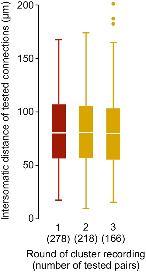
Intersomatic distance distribution Box plots depicting the intersomatic distances of tested connections from rat presubiculum experiments in different clean2extend recording rounds.
Red indicates first round of experiments only utilizing clean2complete strategy (n = 278 pairs). Probed connections after once (n = 218 pairs) or twice (n = 166 pairs) clean2extend are shown in yellow.
Figure 6
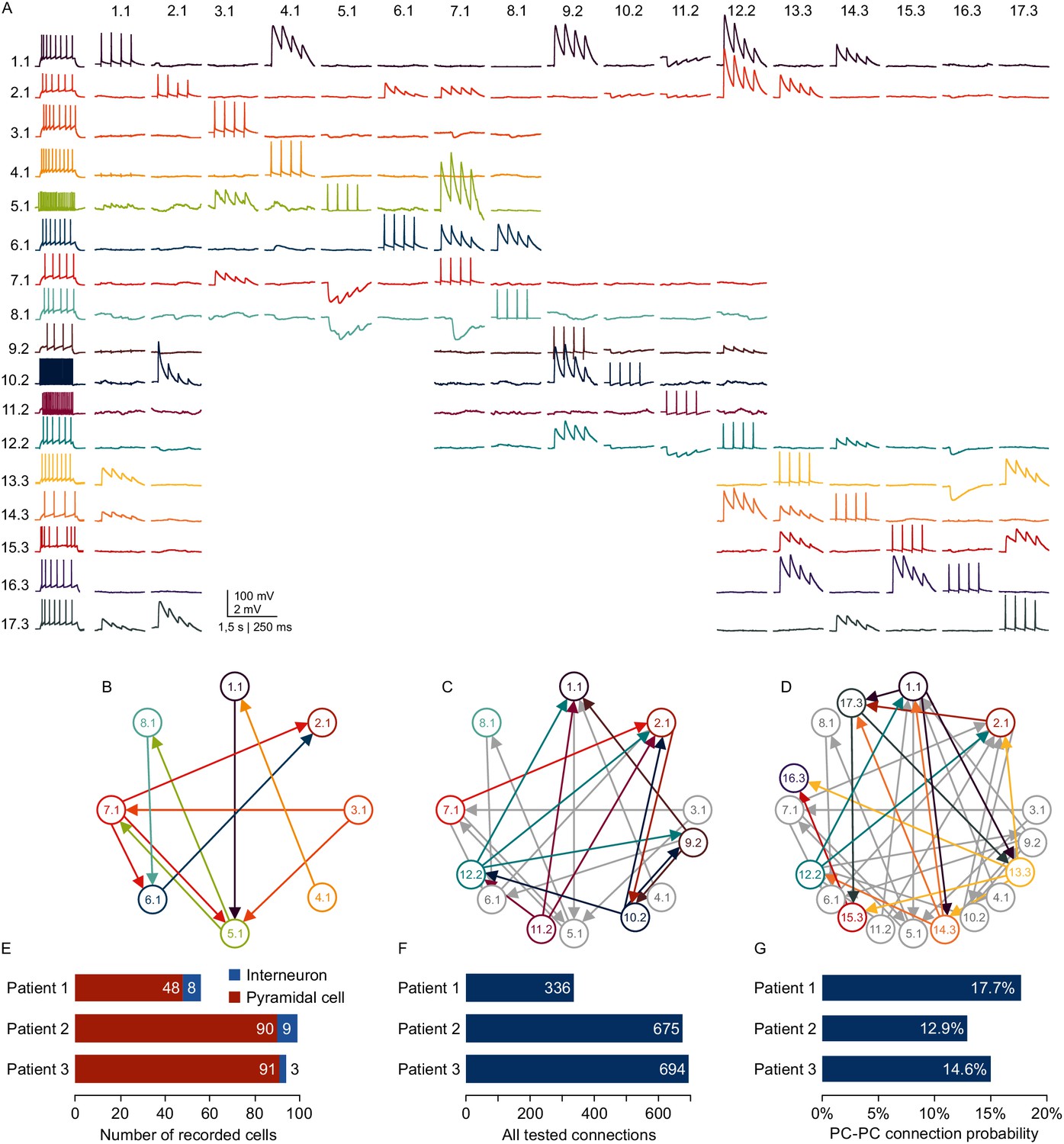
Microcircuit analysis in human slices.
(A) Matrix of averaged voltage traces from 17 neurons in one acute human slice recorded on the -manipulator setup with two rounds of clean-to-extend. Left column shows the firing pattern of the recorded neurons. In the first session eight neurons were patched simultaneously (cells numbered 1.1–8.1). Traces recorded from one cell are shown in a row with the same color. Four action potentials were elicited in each neuron consecutively (diagonal of the matrix). The postsynaptic responses of the other neurons are aligned in the same column. After recording of the first full cluster of 8eight neurons, four pipettes were cleaned and additional neurons in the vicinity were patched and recorded with the same stimulation protocol (9.2–12.2). After the second recording session, another five pipettes were subject to cleaning and five new neurons were patched, while the pipettes on neuron 1.1, 2.1 and 12.2 were not removed. This allowed screening of additional connections among the neurons from the third recording session (13.3–17.3) and also connections between neurons from previous recording sessions (1.1, 2.1 and 12.2). Scale bar: Horizontal 1.5 s for firing pattern, 250 ms for connection screening. Vertical 100 mV for action potentials, 2 mV for postsynaptic traces. (B) Connectivity scheme of all neurons from the first recording session with arrows indicating a detected synaptic connection. (C) Scheme of connections after first cleaning round. Colored arrows and circles indicate neurons and connections recorded in the second session. Neurons and connections of the first recording session are shown in gray. (D) Scheme of all recorded neurons and detected connections after two cleaning rounds. Neurons and connections recorded in this third session are colored. Neurons and connections from previous recording sessions are shown in gray. In this slice, a total of 38 synaptic connections were detected out of 150 tested connections. (E) Bar graphs depicting number of recorded interneurons and pyramidal cells from three patients recorded within the first 24 hr after slicing. (F) Number of tested connections in each patient recorded within the first 24 hr. (G) Connection probability between pyramidal cells calculated by the number of found to tested connections recorded within the first 24 hr. See Figure 6—source data 1.
-
Figure 6—source data 1
Human multipatch.
Rich media files.
- https://cdn.elifesciences.org/articles/48178/elife-48178-fig6-data1-v2.xlsx
Appendix 1—figure 1
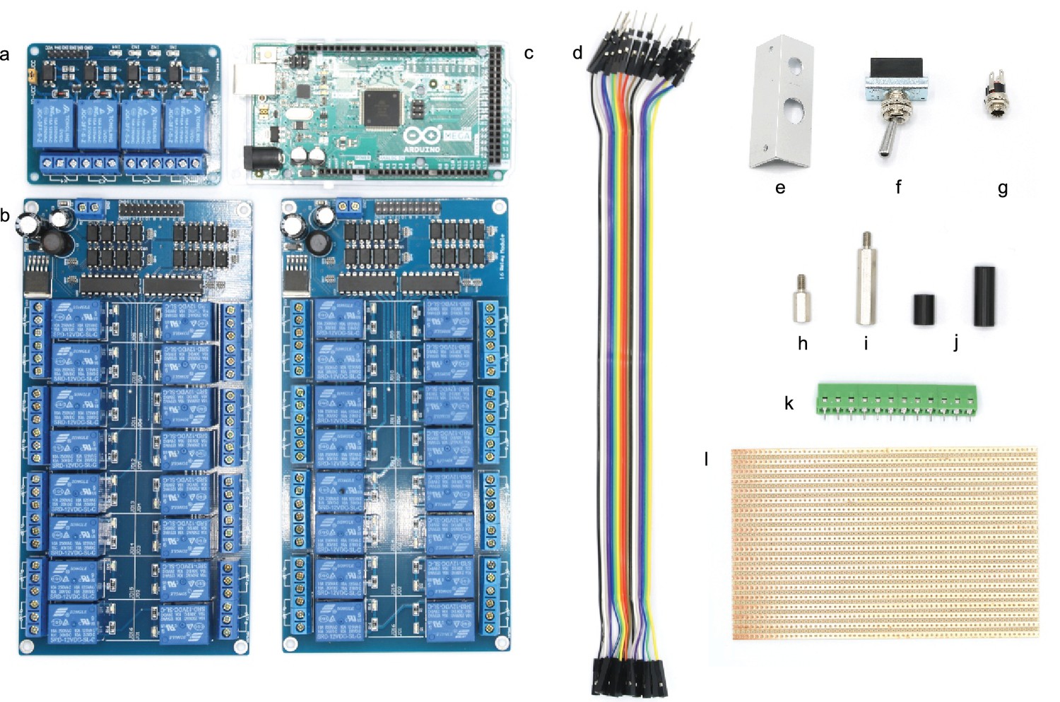
Picture of electronic parts with labelling.
Appendix 1—figure 2
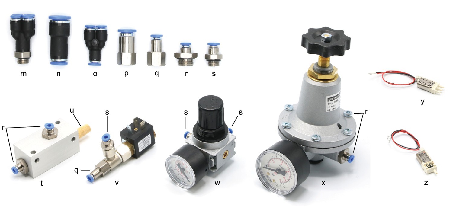
Pictures of pneumatic parts with labelling.
Appendix 1—figure 3
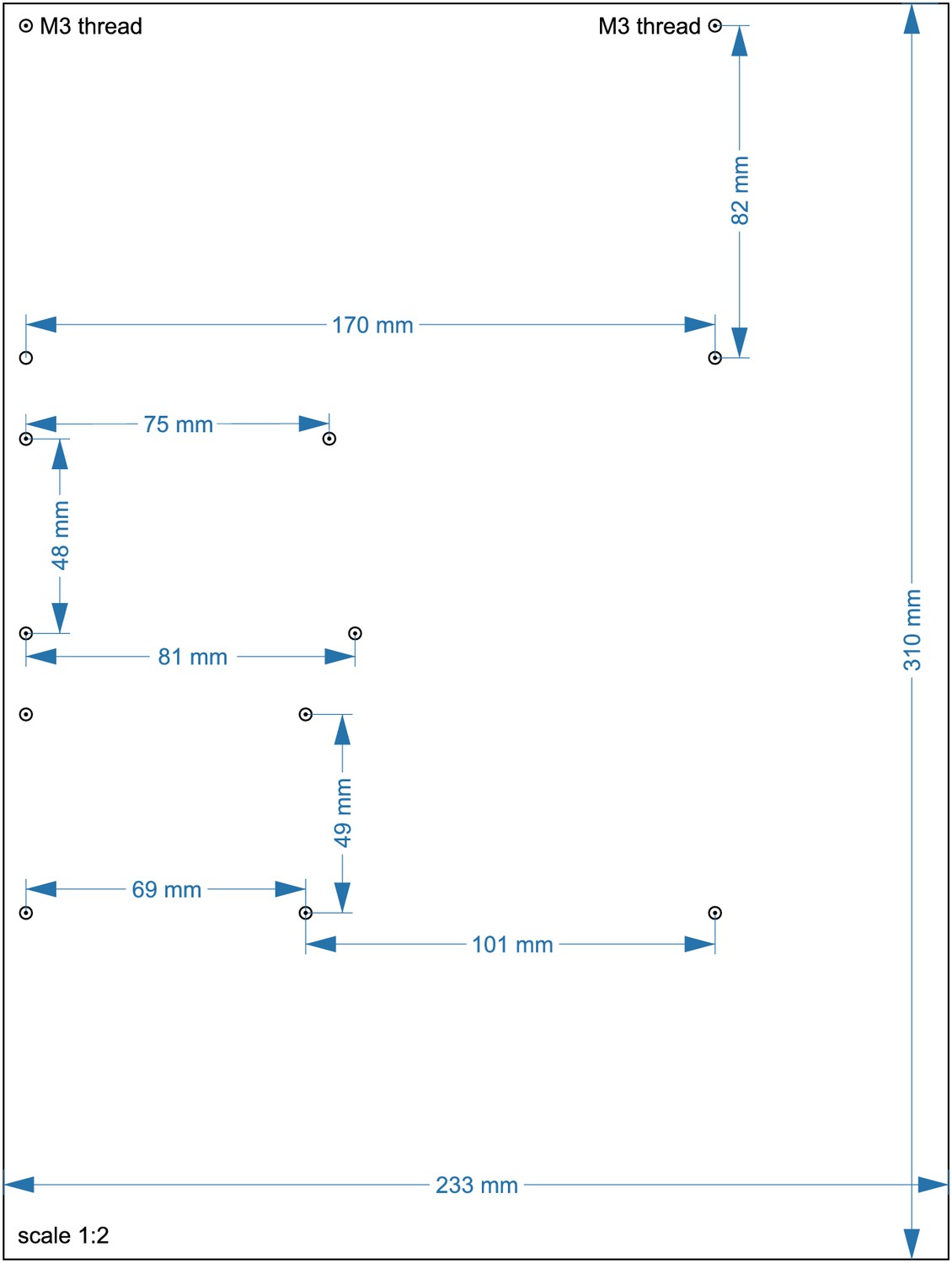
Layout of lower acrylic sheet with 10 mm thickness (13).
Circles indicate positions where a M3 thread needs to be cut. The scale is 1:2, a 1:1 enlarged layout could serve as a printed template.
Appendix 1—figure 4
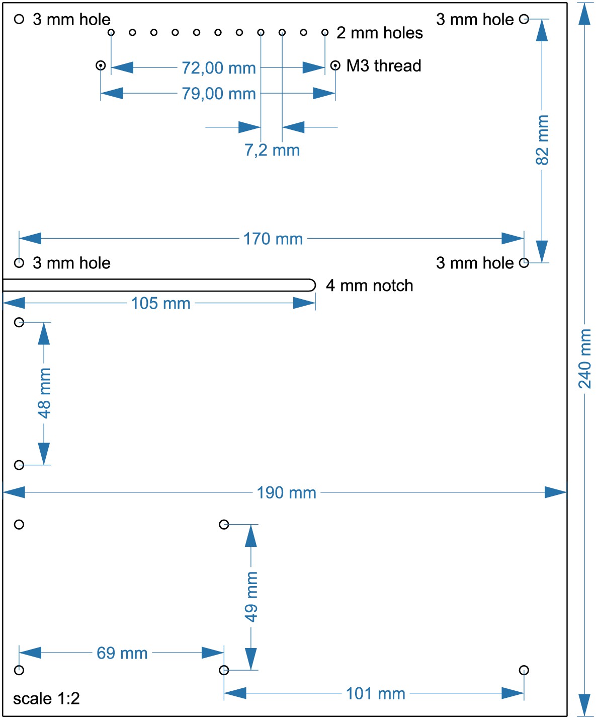
Layout of upper acrylic sheet with 5 mm thickness (14).
Cut 2x M3 threads at circles with spiral. Drill 11 × 2 mm holes, each 7,2 mm apart. All other circles indicate 3 mm holes. A 4 mm notch will allow for passage of cables. The scale is 1:2, a 1:1 enlarged layout could serve as a printed template.
Appendix 1—figure 5
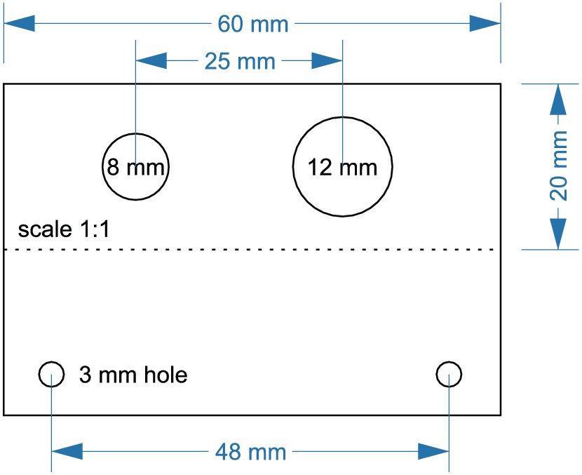
Layout for aluminum angle (5).
Cut the angle at a length of 60 mm. Drill an 8 mm hole for DC barrel connector (7). Drill a 12 mm hole for toggle switch (6). 3 mm holes are needed to attach the angle to the upper plate.
Appendix 1—figure 6
Top: Electrical circuit wiring diagram for valves, relays and Arduino board.
This wiring diagram shows that all solenoid valves (z, v) and the two 16-channel relay board (b) are powered through the 12 V DC power supply (80 W, 12 V / 6,67 A). The 4-channel relay is powered through the Arduino board which receives a 5 V power supply from the USB cable. The gray boxes indicate that this circuit is replicated for each valve in parallel. The relays receive digital signals from the Arduino boards (dotted lines) and switch the contacts from NC (normally closed) to NO (normally open) which brings the solenoid valve into a different state. A flyback diode is necessary for the 2/2 solenoid valves to protect from voltage spikes. Bottom: Photographic wiring scheme of circuit. (1) Ground conductor is connected to all black lines through the soldered screw block on the stripboard (k, l). (2) The 12 V phase conductor (red) is connected to all yellow lines through the other soldered screw terminal block. These yellow wires carry 12 V to power the 16-channel relay board (b), the individual 3/2 solenoid valves (z) and the 2/2 solenoid valves (v). (3) The 4-channel relay board (a) is powered through the 5 V output pin of the Arduino board (c) which is supplied through the USB-cable from the PC.
Appendix 1—figure 7
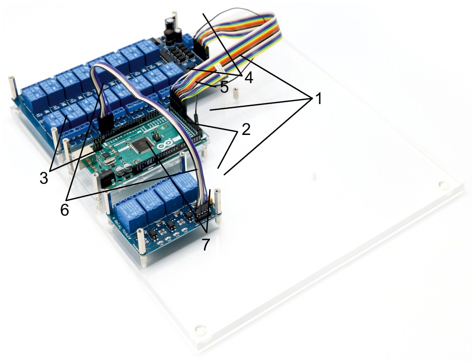
Illustration of step 1-7.
0. Prepare the acrylic sheets.
1. Screw in 10 mm metal spacers (h) in M3 threads of the base plate.
2. Place 16-channel relay (b), 4-channel relay (a) and Arduino Mega (c) on the corresponding positions and fix them with the 25 mm metal spacers (i).
3. The Arduino only needs 2 × 25 mm spacers to fix it.
4. Connect the input pins of the 16-channel relay with digital outputs of the Arduino (e.g. 22–37) using the jumper wire (d) and document the corresponding pin numbers.
5. Connect the ground pins of the 16-channel relay and the Arduino.
6. Connect the input pins of the 4-channel relay with digital outputs of the Arduino (e.g. 10–13) and document the corresponding pin numbers. Also connect the ground pins.
7. Connect the 5V power pin of the Arduino with the VCC pin of the 4-channel relay to power it (cable not shown in picture).
Appendix 1—figure 8
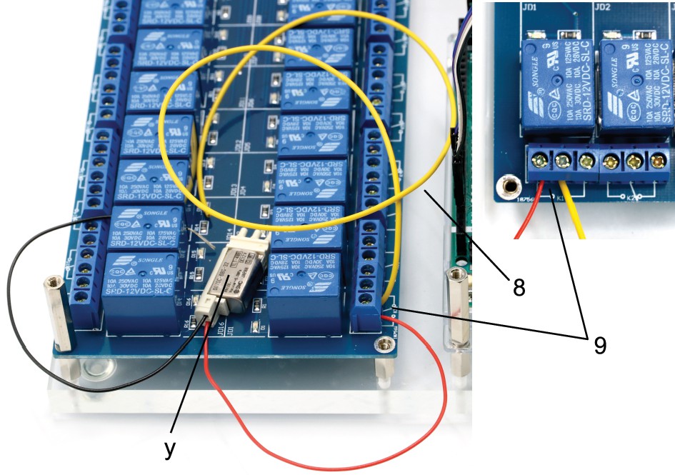
Illustration of step 8-9.
8. Cut 31 yellow isolated copper wires at a length of 15 cm each and strip the ends of the cables.
9. Connect the non-manifold 3/2 solenoid valve (y, S070C-6BG-32) to a relay on the 16-channel relay by connecting the red cable to the normally open contact and connecting the yellow cable to the common contact.
Appendix 1—figure 9
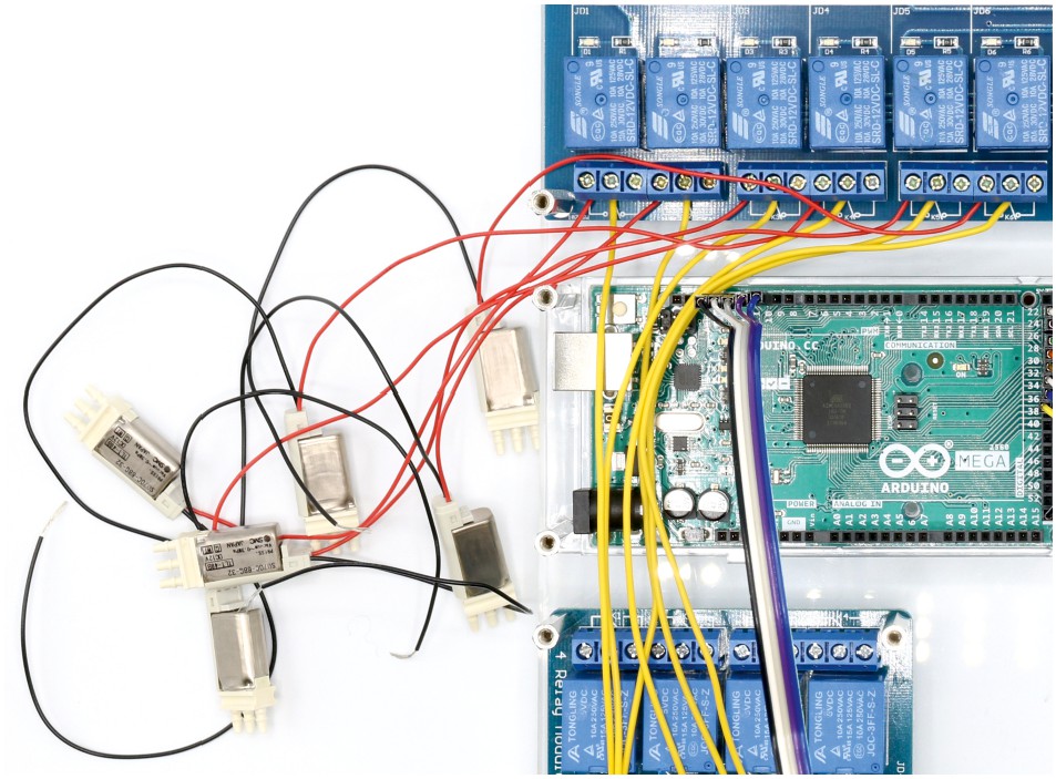
Illustration of step 10.
10. Repeat step 9 with all 11 non-manifold 3/2 solenoid valves (y, S070C-6BG-32). Document which relay is connected to each solenoid valve.
This will be important for the programmed control of each valve in the Matlab code.
Appendix 1—figure 10
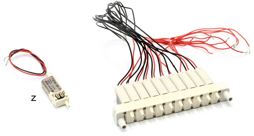
Illustration of step 11.
11. Assemble two arrays of 10 manifold 3/2 solenoid valves (z, S070M-6BG-32) as described in the product information.
Appendix 1—figure 11
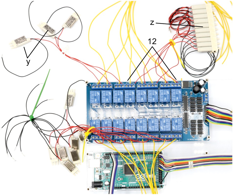
Illustration of step 12.
12. Connect 5 manifold 3/2 solenoid valves (z, S070M-6BG-32) to the remaining relays on the 16-channel relay. Connect the red cable to the normally open contact and the yellow cable to the common contact. Document which relay is connected to each solenoid valve.
Appendix 1—figure 12

Illustration of step 13-14.
13. Attach the second 16-channel relay (b) on top of the other 16-channel relay and fix it with 25 mm spacers (i).
14. Join remaining 5 manifold 3/2 solenoid valves (z, S070M-6BG-32) of the first assembled array with relays of the top 16-channel relay by connecting the red cable to the normally open contact. Connect a yellow cable to the common contact of every relay. Document which relay is connected to each solenoid valve. Pay special attention to order of connections. Intersections of red cables should be avoided. The valve manifold will be oriented as shown in the picture.
Appendix 1—figure 13
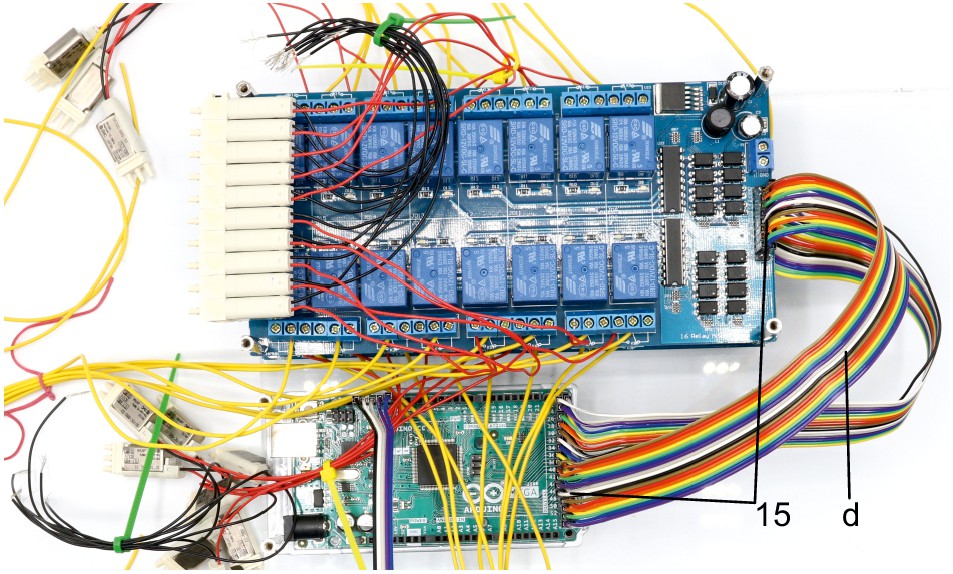
Illustration of step 15.
15. Connect the input pins of the top 16-channel relay with digital outputs of the Arduino (e.g. 38–53) using the jumper wire (d) and document the corresponding pin numbers. Connect the ground pins of the 16-channel relay and the Arduino.
Appendix 1—figure 14
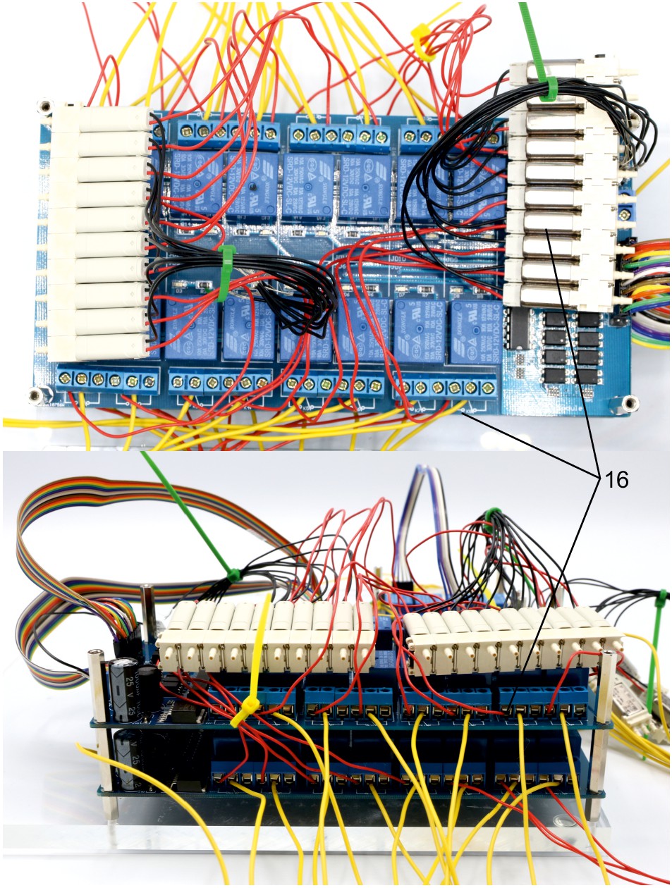
Illustration of step 16.
16. Assemble second array of ten manifold 3/2 solenoid valves (z, S070M-6BG-32) and connect these to relays of the top 16-channel relay by connecting the red cable to the normally open contact. Document which relay is connected to each solenoid valve.
Appendix 1—figure 15

Illustration of step 17-20.
17. Solder red and black wires (approx. 10 cm) to contacts of 3 × 2/2 solenoid valves (v).
18. Include a diode (1N4007) between the contacts to avoid current from capacitor discharge damaging the remaining circuit.
19. Connect 2/2 solenoid valves to the 4-channel relay. Connect the red cable to the normally open contact and a yellow cable (approx. 10 cm) to the common contact. Document which relay is connected to each solenoid valve.
20. Screw on push-in fittings (s, q) onto the 2/2 solenoid valves.
Appendix 1—figure 16
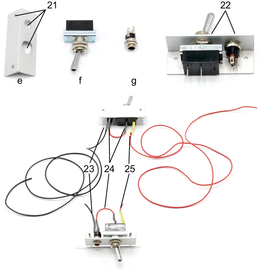
Illustration of step 21-25.
21. Drill holes (3, 8, 12 mm) in aluminium angle (e) as shown on the layout.
22. Attach the toggle switch (f) to the 12 mm hole and the DC barrel power connector (g) to the 8 mm hole.
23. Solder a black wire (approx. 10 cm) to the neutral conductor of the power connector. This wire will connect to all ground wires (black wires) of the valves and relays.
24. Solder a red wire to the DC conductor of the power connector and to a contact of the ON/OFF switch.
25. Solder another red wire (approx. 10 cm) to the other contact of the toggle switch. This wire will condcut 12V for all valves and relays (yellow wires).
Appendix 1—figure 17
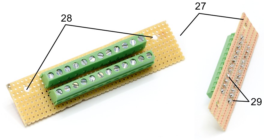
Illustration of step 27-29.
27. Cut the stripboard to a 25 × 95 mm rectangle with longitudinal orientation of the conducting striples.
28. Drill two 3 mm holes, 82 mm apart and 7 mm away from the edge. This stripboard will be fixed onto the top acrylic plate above the 16-channel relays.
29. Solder both screw terminal blocks (k) onto the stripboard so that all contacts of one block are connected.
Appendix 1—figure 18
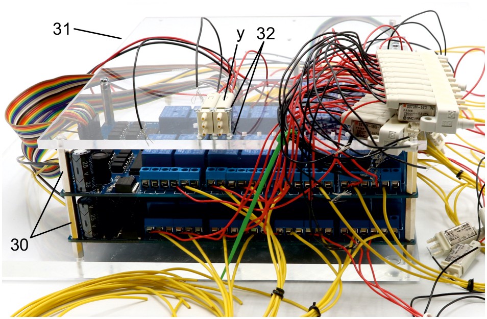
Illustration of step 30-32.
30. Screw in second 25 mm metal spacer (i) on top of all metal spacers to create level pillars of metal spacers for the upper acrylic plate.
31. Mount upper acrylic plate (5 mm) on top of the 25 mm metal spacers (i).
32.Use 20 mm M2 bolts to attach the non-manifold 3/2 solenoid valves (y) at the location of the 2 mm holes on the upper acrylic plate. Use M2 nuts below the acrylic plate to fix the valves.
Appendix 1—figure 19
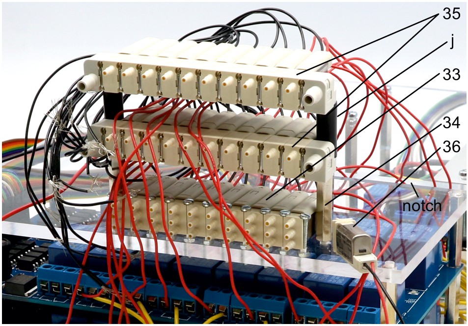
Illustration of step 33-36.
33. Repeat step 32 for 10 of the 11 non-manifold 3/2 solenoid valves (z). Document position of each valve, their respective relay and connected Arduino digital output pin.
34. Screw in two 25 mm metal spacers (i) next to the first level of non-manifold solenoid valves.
35. Attach the other two solenoid valve manifolds (z) on top of the metal spacers separated by 20 mm plastic spacers (j) and fixed using 35 mm M3 bolts. Pay attention to avoid twisting of the cables. Route the cables either through the notch or around the upper plate.
36. The 11. non-manifold solenoid valve is later attached on the top plate.
Appendix 1—figure 20
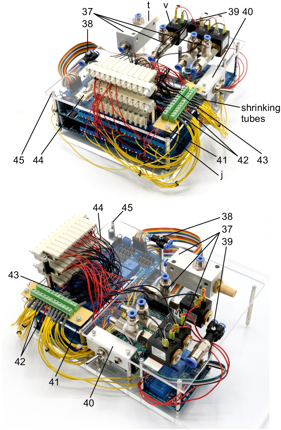
Illustration of step 37-45.
37. Attach vacuum ejector (t), equipped with G1/4 push-in fittings (r) and silencer (u), and three 2/2 solenoid valves (v), equipped with G1/8 push-in fittings (s, q), onto the top plate using double-sided adhesive tape.
38. Use 25 mm M3 bolt to attach the push-in Y-fitting (o).
39. Use 35 mm M3 bolt to attach the multiple distributor with four outlets (m, p).
40. Attach the angle with toggle switch and DC power connector (step 21–25) underneath the top acrylic plate, above the Arduino and use M3 bolts to fix it.
41. Attach the cut stripboard with soldered screw terminal blocks (step 27–29) to the top plate using two 25 mm M3 bolts and two 10 mm plastic spacers (j).
42. Connect all yellow wires from the relays and the 16-channel relay boards to one screw terminal block which also connects the red 12V phase conductor from the toggle switch (step 25). This distributes the 12V power from the DC power connector to the relays and thereby to the solenoid valves through the red wires.
43. Connect all black neutral wires from the solenoid valves and the 16-channel relay boards to the other screw terminal block which is also connected with the black neutral conductor wire from the DC power connector (step 23).
44. Use double-sided adhesive tape to attach the 11. non-manifold solenoid valve (step 36) onto the top plate, adjacent to other 3/2 solenoid valves.
45. Use 10 mm M3 bolts on remaining holes.
Appendix 1—figure 21
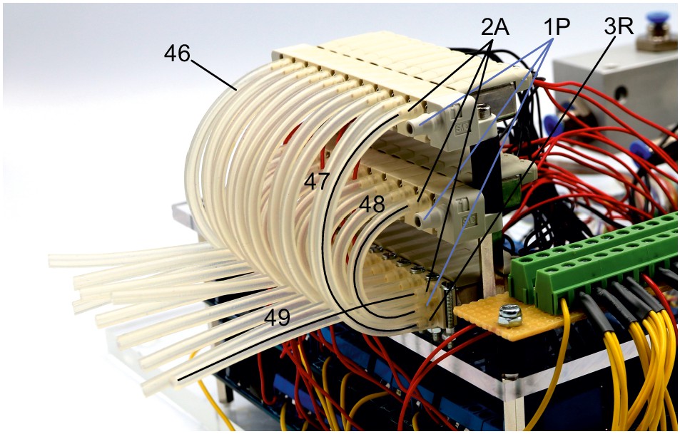
Illustration of step 46-49.
The following steps connects the 3/2 valves to enable application of different pressures to individual pipette holders.
For schematic depiction, please see respective figure.
46. Cut 10 silicon tubes (diameter 2/4 mm) with a length of 9.5 cm, 10 silicon tubes with a length of 6 cm and 10 silicon tubes with a length of 8 cm.
47. Connect one end of the 9.5 cm tubes to the 2A nozzle of the top level valves and the other end to the lower 3R nozzle of the respective first level valves.
48. Connect one end of the 6 cm silicon tubes to the 2A nozzle of the second level valves and the other end to the middle 1P nozzle of the respective first level valves.
49. Connect one end of the 8 cm tubes to the top 2A outlets of the first level valves. The other end can be connected to tubes that directly connect to the respective pipette holders.
Appendix 1—figure 22
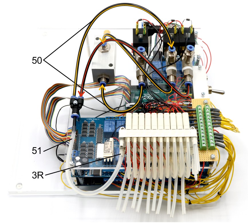
Illustration of step 50-51.
The following steps connects the 2/2 valves and vacuum ejector to the 3/2 valve manifolds to generate the necessary pressures for the cleaning procedure.
The tubes highlighted in red transfer the 1 bar positive pressure. The tubes highlighted in yellow transfer the negative pressure for suction. Arrowheads indicate direction of air flow.
50. Connect the PE-tubes (outer diameter 4 mm, inner diameter 2 mm) as shown between the 2/2 valves and the vacuum ejector. Connect these to the Y-fitting.
51. Connect the Y-fitting to the 3R nozzle of the second level 3/2 valve manifold through a silicone tube (diameter 4/6 mm).
Appendix 1—figure 23
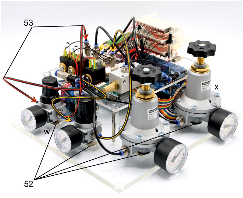
Illustration of step 52-43.
The following steps connect the 1–10 bar pressure regulators (w) to the pressurized air supply and the 2/2 solenoid valves.
52. Position the pressure regulators (w, x) on the base plate and fix them using double sided adhesive tape. We found this to be of sufficient stability. Pay special attention to the intended direction of air flow depicted on the regulators.
53. Connect the PE-tubes to the multiple distributor with four outlets and to the 1–10 bar pressure regulators (w). Then connect those to the 2/2 solenoid valves as depicted. Meaning of color code and arrowheads correspond to the previous steps.
Appendix 1—figure 24
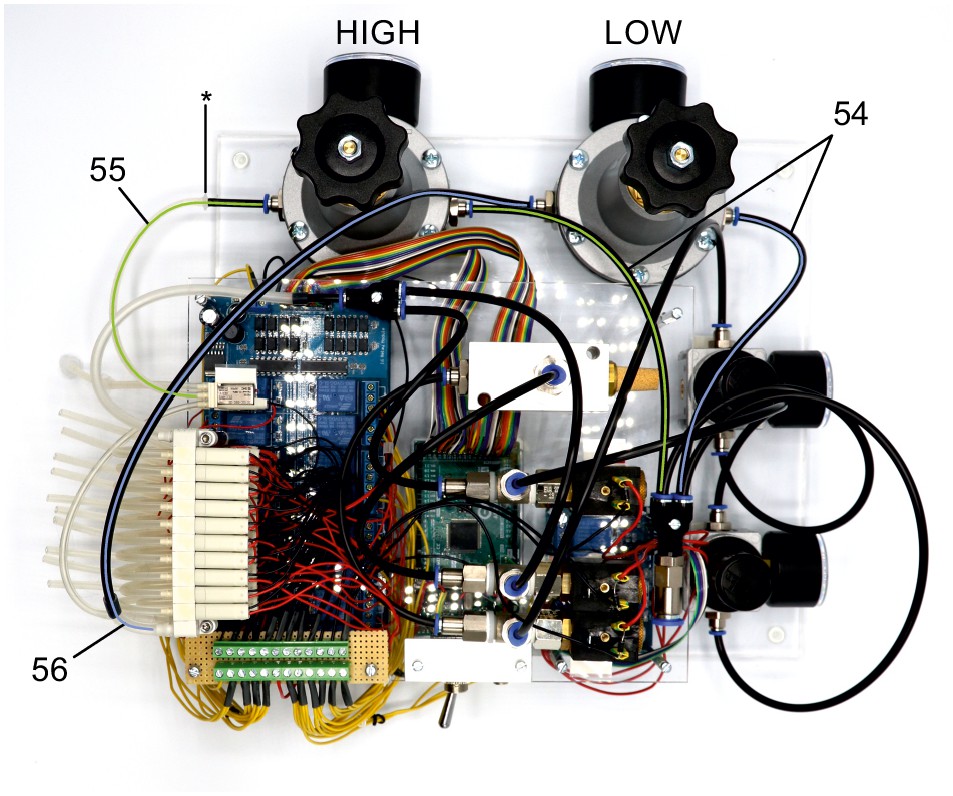
Illustration of step 54-56.
The following steps connect the precision pressure regulators (x, 10–1000 mbar) to the valve manifold to generate HIGH pressure (70 mbar, green lines) and LOW pressure (20 mbar, blue lines).
54. Connect 2 PE-tubes to the multiple distributor with four outlets and each to one of the precision regulators. Pay spetial attention to intended direction of airflow on the regulators. Arrowheads indicate direction of air flow.
55. Connect the HIGH pressure regulator (set to 70 mbar) to the middle nozzle of the single 3/2 solenoid valve which is attached to the acrylic plate (green line). Connect the PE-tubing with a 2/4 mm silicone tube using a mini tubing connector(*).
56. Connect the LOW pressure regulator (set to 20mbar) to the 1P nozzle of the top level 3/2 valve manifold. Use a 4/6 mm silicone tube to connect the PE-tubing with the nozzle.
Appendix 1—figure 25

Illustration of step 57-58.
57. Connect the 1P nozzle of the second level solenoid valve manifold to the 3R nozzle of the single 3/2 solenoid valve. Use a 4/6 mm silicone tube to connect the 1P nozzle of the manifold. Connect it with a 2/4 mm silicone tube using a mini tubing reducer.
58. Connect a 2/4 mm silicone tube to the 2A nozzle of the single 3/2 solenoid valve which can be connected to a mouth piece or a syringe for applying pressure during membrane sealing and breakthrough.
Appendix 1—figure 26
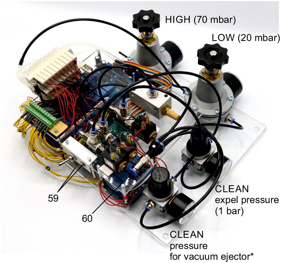
Illustration of step 59-60.
59. Plug in the power supply (12 V / 6.67 A, 80 W) and the USB-cable to the Arduino board.
60. Connect to presurrised air supply using a PE-tubing with 8 mm outer diameter. The air supply should be set at sufficient high pressures (e.g. 5 bar).
Adjust the regulators manually to the desired pressures.
*The pressure regulator upstream of the vacuum ejector needs to be adjusted while measuring the negative pressure generated by the vacuum ejector. It should be set at a pressure at which −350 mbar can be applied to the valve manifold (approx. 3–5 bar). To control the device, you can use the Matlab code and GUI we provided. One could also control the Arduino board using any custom script. Before the first use, please transfer the mapping of the individual valves onto their relay number and respective Arduino digital output pin into the script (see guide to Matlab GUI). Now the pressure control device is fully operational.
Appendix 1—figure 27
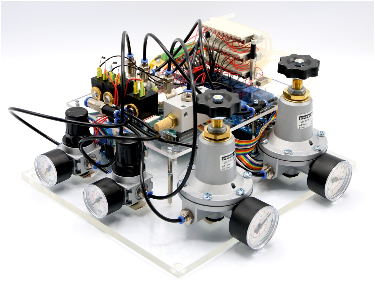
Photograph of finished pressure system.
Appendix 2—figure 1
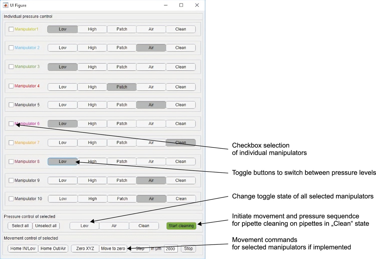
Screenshot of MATLAB graphical user interface to control pressure levels and cleaning sequence.
Appendix 2—figure 2
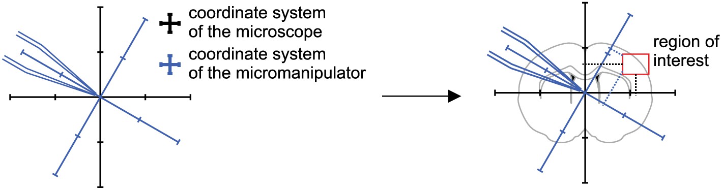
Coordinate transformation.
Calculate coordinates of micromanipulator corresponding to coordinates of the microscope.
Appendix 2—figure 3

Move pipette to calculated coordinate.
Appendix 2—figure 4
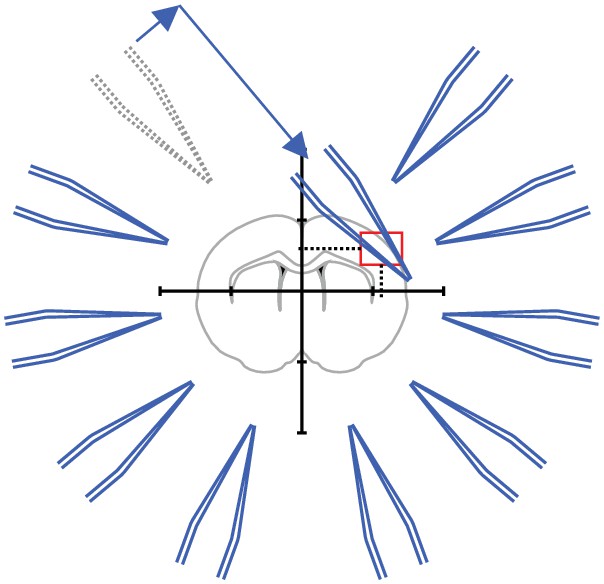
Step 1: A brain slice is placed under the microscope.
The ‚region of interest ‘is located in the coordinate system of the microscope.
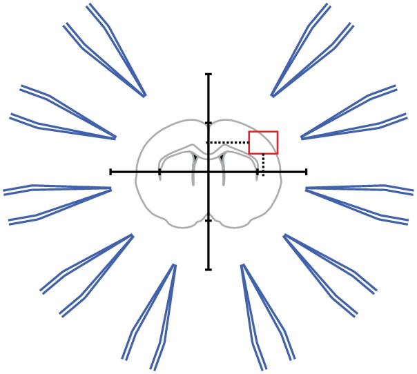
Appendix 2—figure 5

Step 2: The coordinates of the ‚region of interest ‘are fed into the pipette finding algorithm.
The coordinates for each manipulator are computed.
Appendix 2—figure 6
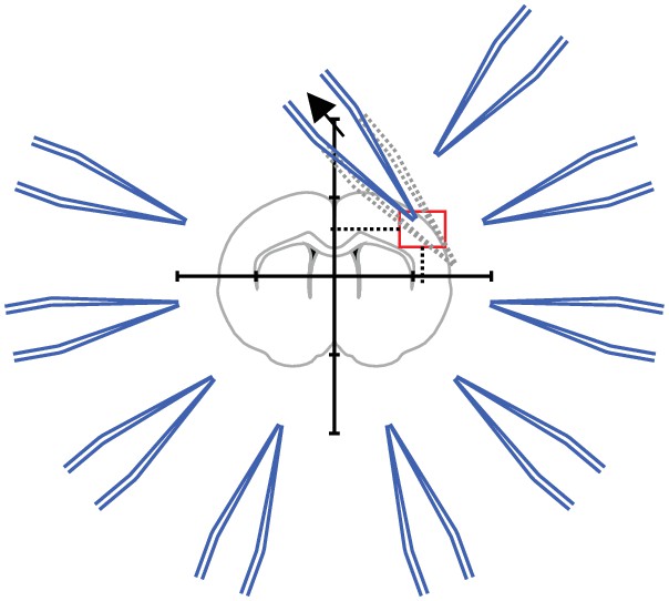
Step 3: Pipette one is moved to the calculated coordinate.
Manual adjustments are necessary to due variations in pipette shape.
Appendix 2—figure 7
Step 4: Pipettes should be moved to a designated corner that will prevent collisions with the other pipettes.
This position is then saved.
Appendix 2—figure 8
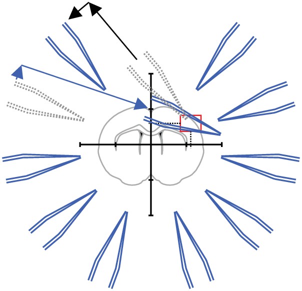
Step 5: The pipette is moved to its starting position while the next pipette is moved to the position calculated by the pipette finding algorithm.
Repeat step 4 and step five for all manipulators.
Appendix 2—figure 9
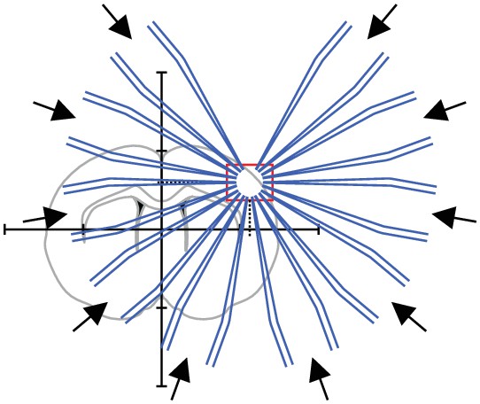
Step 6: All pipettes are moved to their target positions simultaneously.
All pipttes are now positioned in the region of interest.
Appendix 3—figure 1
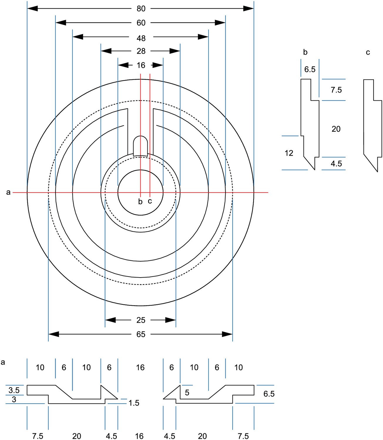
Drawing of recording chamber for Scientifica manipulators.
All measurements in mm. Dotted lines = edges on underside.
Appendix 3—figure 2
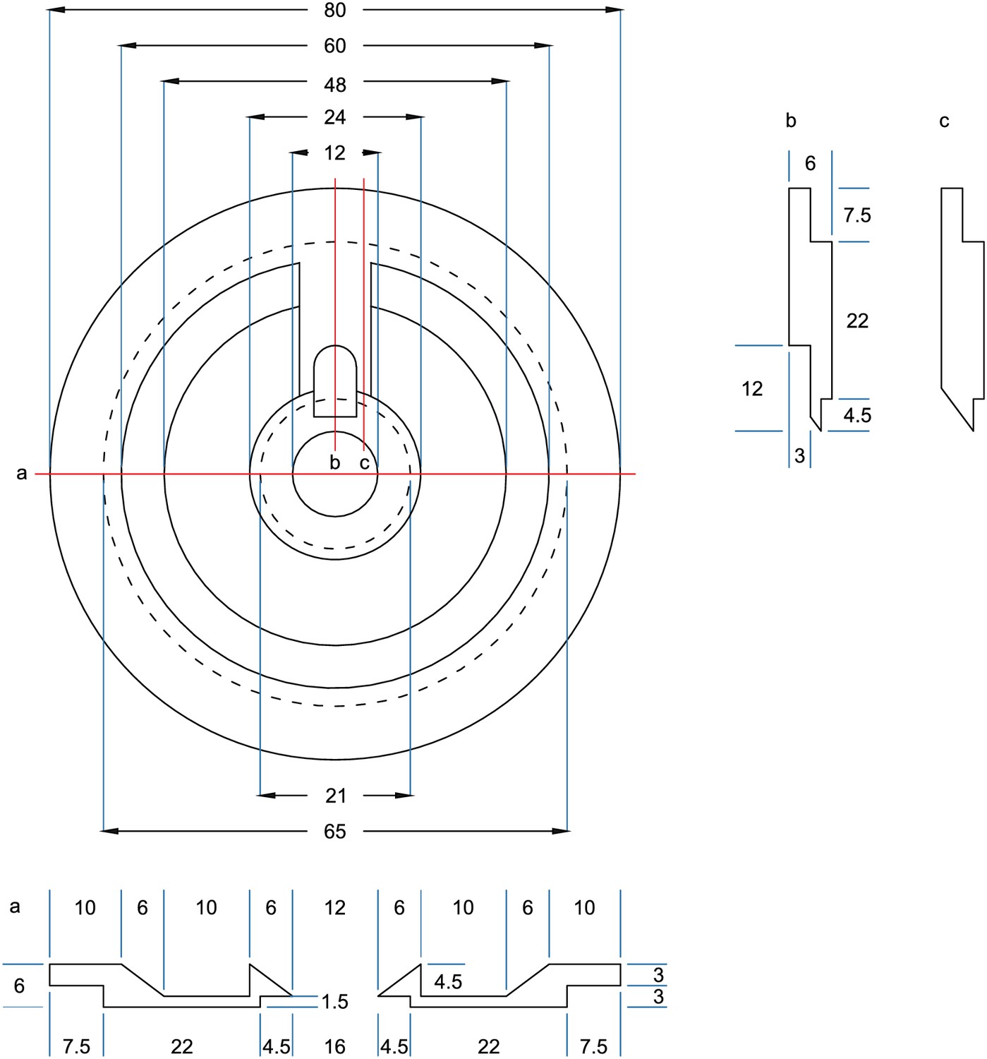
Drawing of recording chamber for Sensapex manipulators.
All measurements in mm. Dotted lines = edges on underside. Adjustments are needed for Sensapex micromanipulators. Due to a range of motion in the axial axis of 20 mm, the real horizontal range of motion is less than 20 mm. Therefore, the central recording well has a smaller diameter.
Appendix 3—figure 3
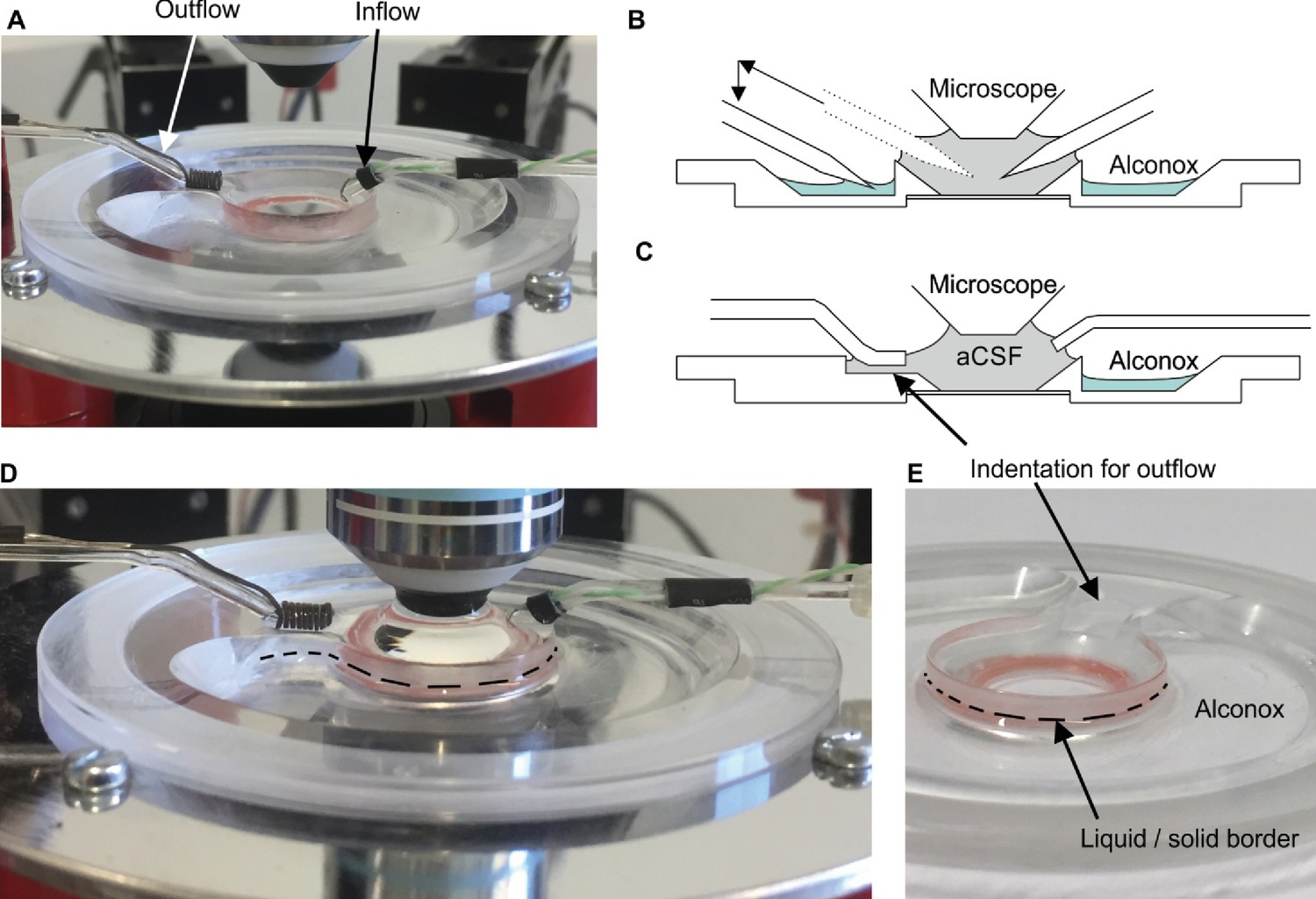
Illustration of recording chamber and solutions.
(A) Photograph of recording chamber with inflow and outflow placed into the central well. (B) Schematic view of pipettes in the central well. The left pipette is moved from the center well into the outer circular well containing Alconox. (C) Schematic view of in- and outflow. Note that outflow is placed in the indentation which guarantees a constant liquid level in the recording chamber. (D) The inflow is placed in the aCSF. Black dashed lines indicate the liquid/solid border. (E) Close up view of the liquid/solid border.
Appendix 3—figure 4
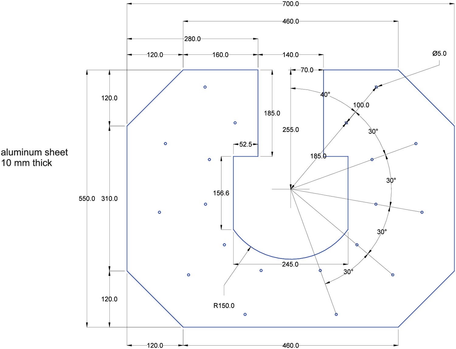
10 mm thick sheet of aluminum.
The sheet is shown in blue. Measurements are shown in black. All measurements are in milimeters. All drilling-holes are 5 mm in diameter (for M6 ISO metric screw threads).
Appendix 3—figure 5
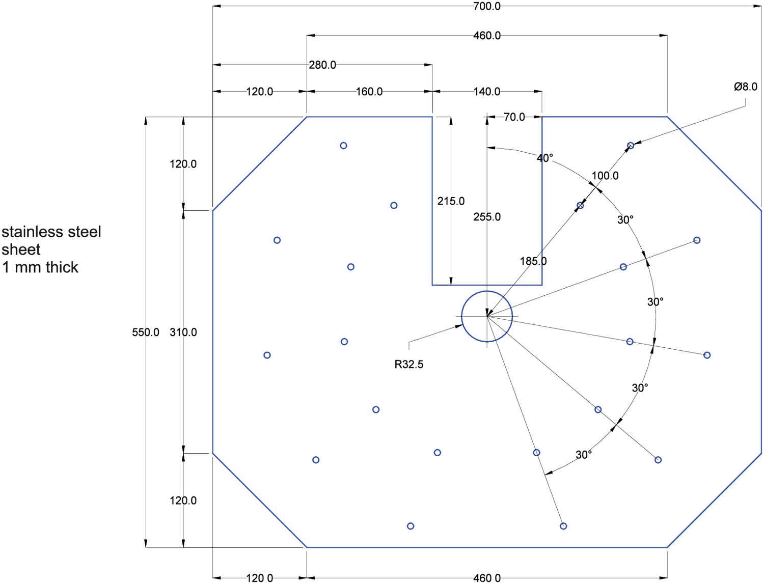
1 mm thick sheet of stainless steel.
The sheet is shown in blue. Measurements are shown in black. All measurements are in milimeters. All holes in the stainless steel sheet are 8 mm in diameter. The two sheets have to be glued together before being mounted into the setup with the stainless steel sheet facing upwards.
Appendix 3—figure 6

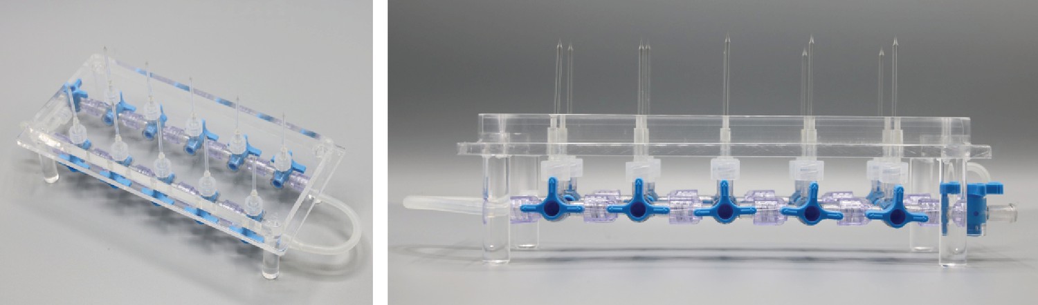
Photographic overview of multi-pipette filling device.
Appendix 3—figure 7
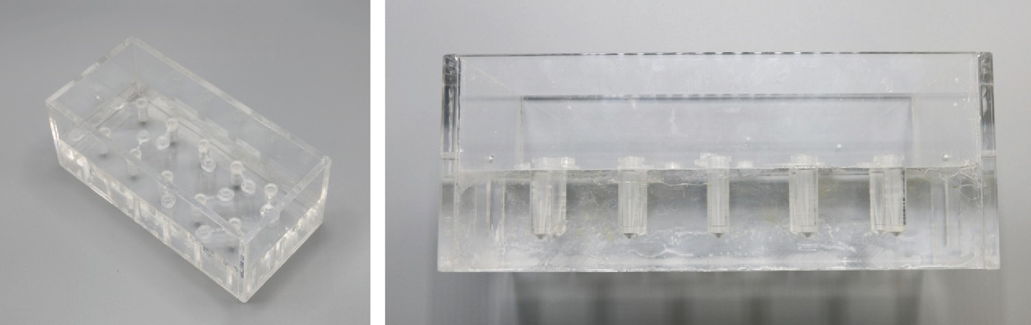
Bottom part.
Appendix 3—figure 8
Top part.
Appendix 3—figure 9
Bottom part of pipette filling station.
1,5 ml microcentrifuge tubes with intracellular solution are inserted into the 8 mm holes. Slight adjustment might be necessary to guarantee upright position of the tubes and easy insertion. Distance between the holes (32 mm) are determined by the distance of the central channel between two connected Braun 3-way stopcocks. Slight variation might be necessary when different models are chosen. Height of the walls are determined by the length of the pipettes to ensure that pipettes will reliably dip into the tubes. The current measurements are optimized for approximately 40 mm long pipettes.
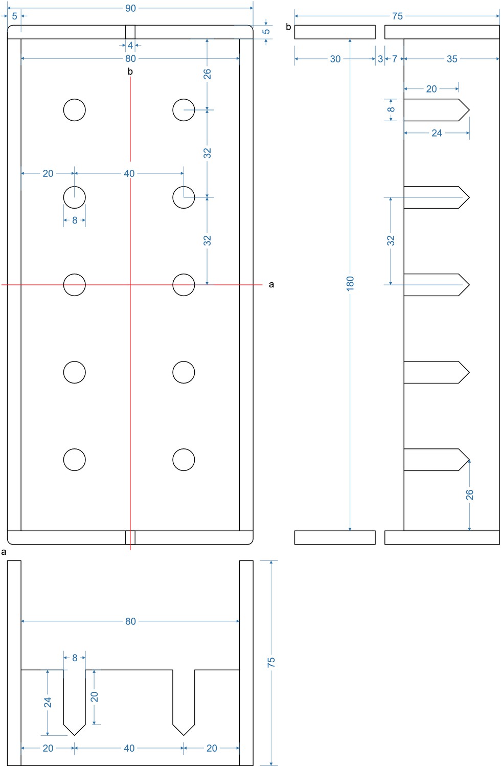
Appendix 3—figure 10

Top part of pipette filling station (‘lid’).
Pipettes will be inserted into the 2,5 mm holes. Silicon tubes with 1,5 mm inner diameter and 3,5 mm outer diameter will be inserted into the 4 mm holes until the narrowing. Section (a) depicts the horizontal section through the middle depicting the 2 mm and 4 mm holes. Section (b) depicts a longitudinal section through the pillars of the lid. These enable a stable upside-down positioning of the lid in which the pipettes will be pointing upwards. The pillars are glued into a 10 mm hole.
Appendix 3—figure 11
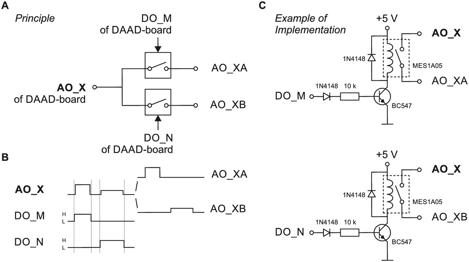
Schematic wiring diagram for analog output routing device.
(A) Principle of a very simple and limited analog-out-switch distributing the analog out signal of the DAAD´s analog output channel AO_X to two channels serving two amplifiers or amplifier channels. The switches are gated by digital output channels of the DAAD-board (DO_M and DO_N). (B) Via AO_X two different, non-simultaneous, non-overlapping command signals (different time of occurence, amplitude, duration) are sent to the switch, DO_M and DO_N are set high (H) as indicated (note that the digital pulses should start slightly earlier and terminate slightly later than the intended analog signals) and thus gate the respective command to the respective output of the switch (AO_XA or AO_XB). This switch is limited in the sense that the connected AO_XA and AO_XB will carry an identical (voltage- or current-) command signal (technically in both cases a voltage signal) from the DAAD to the individual amplifier inputs if command signals are to be applied simultaneously. (C) Example of implementing the principle shown in A. To distribute the analog out command signal of the DAAD-board to two amplifier command input channels, two reed relais (e.g. MES1A05) are used. The power supply can be taken from an USB-port of a computer.
Videos
Video 1
Automated cleaning of all pipettes on a 10-multipatch setup.
The main image depicts a front view of the 10-manipulator setup with all manipulators subject to automated movements during a pipette cleaning sequence. The insert on the bottom left corner shows a close-up view of the pipettes and the recording chamber. For better overview, the two front manipulators were moved aside. The insert on the bottom right corner shows the DIC microscope view with a 4x objective. At the end of the sequence, all pipettes are out of focus, due to different final z-positions. The time stamp in the middle shows the elapsed time in seconds. Roughly 20 s of alternating pressure sequence was cut (second 13 to 32). The last 8 s sequence shows the pressure system while switching between pressure levels. The clicking noise is generated by the relais switches.
Video 2
Pipette positioning algorithm.
This video shows the pipette movements during the positioning phase under the DIC microscope. The first sequence is in a 5x time lapse with the 4x objective. Pipettes are moved in and out automatically, note the small manual adjustments in between. The second sequence is played in real time and shows all pipettes moving to their adjusted target position underneath the 40x objective.
Tables
Table 1
Hardware components of 10-manipulator setup.
| Hardware | Manufacturer | Model |
|---|---|---|
| five dual patch-clamp amplifiers | Molecular Devices | MultiClamp 700B CV-7B headstage |
| Data acquisition system | Cambridge Electronic Design | Power1401-3A + Signal Expansion (2701–5) |
| Stimulation routing device | Custom-made | Design in supplement |
| 10 Micromanipulators | Sensapex | u-Mp Micromanipulator |
| Microscope | Nikon | Eclipse FN1 |
| Motorized stage for microscope | Scientifica | UMS-2550P for x-/y-axis Stepper motor for z-axis drive |
| Camera | Hamamatsu | Orca-Flash 4.0 |
| LED infrared light source | Thorlabs | M780L3 |
| four height adjustable poles | Thorlabs | P250/M, PB1, C1515/M |
| Active vibration isolation table | Accurion | Halcyonics_i4large |
| Peristaltic pump | Gilson | Minipuls 3 |
| Thermostat | Multichannel systems | TC01 |
| Stage for manipulators | Custom-made | Design in supplement |
| Recording chamber | Custom-made | Design in supplement |
Appendix 1—table 1
Table of electronic parts referring to Appendix 1—figure 1 including part number and cost.
| # | Electronic parts | Amount/pieces | Supplier/producer* | Part number* | Unit cost €* | Total cost €* |
|---|---|---|---|---|---|---|
| a | 4-channel relay board 5 V | 1 | sertronics | RELM-4 | 3.19 | 3.19 |
| b | 16-channel relay board 12 V | 2 | sertronics | RELM-16 | 16.72 | 33.45 |
| c | Arduino Mega 2560 microcontroller | 1 | reichelt | ARDUINO MEGA | 26.81 | 26.81 |
| d | 20 position male to female jumper wire, 20 cm length | 2 | reichelt | DEBO KABELSET | 3.24 | 6.47 |
| power supply 80W, 12 V / 6,67 A | 1 | reichelt | MW GST90A12 | 25.59 | 25.59 | |
| e | aluminium angle 20 × 20×2 mm | 20 cm | alusteck | W20202 | 1.58 | 1.58 |
| f | ON/OFF switch, 250 V / 6 A | 1 | reichelt | MAR 1821.1101 | 1.67 | 1.67 |
| g | DC barrel power connector, 2.5 mm center pole diameter | 1 | reichelt | HEBL 25 | 0.34 | 0.34 |
| h | metal spacer hexagonal, male/female M3, 10 mm | 14 | reichelt | DA 10 MM | 0.11 | 1.53 |
| i | metal spacer hexagonal, male/female M3, 25 mm | 24 | reichelt | DA 25 MM | 0.17 | 4.03 |
| j | plastic spacer, M3, 10 mm | 4 | reichelt | DK 10 MM | 0.03 | 0.12 |
| j | plastic spacer, M3, 20 mm | 2 | reichelt | DK 20 MM | 0.03 | 0.06 |
| k | screw terminal block, PCB mount, 12 pole | 6 | reichelt | RND 205–00242 | 0.83 | 4.99 |
| l | stripboard, pitch corresponding to screw terminal | 2 | reichelt | H5SR160 | 1.35 | 2.69 |
| acrylic plate, 31 × 27 cm, 10 mm thickness | 1 | Express- zuschnitt | AGS-100-TRA | 11.20 | 11.20 | |
| acrylic plate, 24 × 19 cm, 5 mm thickness | 1 | Express-zuschnitt | AGS-50-TRA | 5.97 | 5.97 | |
| hexagonal nut, M3 | 100 | reichelt | SK M3 | 0.83 | 0.83 | |
| hexagonal nut, M2 | 100 | reichelt | SK M2 | 1.81 | 1.81 | |
| bolt, M2, 20 mm | 100 | reichelt | SZK M2 × 20 | 7.90 | 7.90 | |
| bolt, M3, 10 mm | 100 | reichelt | SZK M3 × 10 | 1.60 | 1.60 | |
| bolt, M3, 25 mm | 100 | reichelt | SZK M3 × 25 | 2.27 | 2.27 | |
| bolt, M3, 35 mm | 100 | reichelt | SZK M3 × 35 | 3.78 | 3.78 | |
| plain washer, 3.2 mm | 100 | reichelt | SKU 3,2 | 0.92 | 0.92 | |
| isolated copper wire, 0.14 mm², yellow | 20 m | reichelt | LITZE GE | 1.28 | 1.28 | |
| isolated copper wire, 0.14 mm², red | 20 m | reichelt | LITZE RT | 1.28 | 1.28 | |
| isolated copper wire, 0.14 mm², black | 20 m | reichelt | LITZE SW | 1.31 | 1.31 | |
| USB-A to USB-B 2.0 cable | 5 m | reichelt | DELOCK 83896 | 3.31 | 3.31 |
-
*The reported part numbers and prices are from German suppliers in 2017. Equipment necessary for soldering, drilling holes and making threads are not listed.
Appendix 1—table 2
Table of pneumatic parts referring to Appendix 1—figure 2 including part number and cost.
| # | Pneumatic parts | Amount | Supplier/ Producer* | Part number* | Unit cost €* | Total cost €* |
|---|---|---|---|---|---|---|
| m | push-in fitting, multiple distributor four outlets, G1/8 external thread, 4 mm tubing | 1 | Esska | IQSQ184G0000 | 3.29 | 3.29 |
| n | push-in reducing connector, 10 mm/8 mm tubing | 1 | Esska | IQSG10800000 | 2.25 | 2.25 |
| o | push-in Y-fitting, 4 mm tubing | 1 | Esska | IQSY40000000 | 1.50 | 1.50 |
| p | push-in fitting, G1/8 internal thread, 8 mm tubing | 1 | Esska | IQSF18800000 | 1.62 | 1.62 |
| q | push-in fitting, G1/8 internal thread, 4 mm tubing | 3 | Esska | IQSF18400000 | 1.64 | 4.92 |
| r | push-in fitting, G1/4 external thread, 4 mm tubing | 6 | Esska | IQSG144G0000 | 1.08 | 6.48 |
| s | push-in fitting, G1/8 external thread, 4 mm tubing | 7 | Esska | IQSG184G0000 | 0.96 | 6.72 |
| t | vacuum ejector | 1 | Esska | 175811211 | 70.26 | 70.26 |
| u | silencer for vacuum ejector | 1 | Esska | SD14MS000000 | 1.06 | 1.06 |
| v | 2/2 solenoid valve | 3 | Esska | 8552MZ12V000 | 32.14 | 96.42 |
| w | pressure regulator, 1–10 bar | 2 | Esska | R018-6000000 | 29.85 | 59.70 |
| x | precision pressure regulator, 10–1000 mbar | 2 | Esska | DRF31GS00000 | 68.38 | 136.76 |
| y | 3/2 solenoid valve, body ported | 12 | SMC | S070C-6BG-32 | 38.04 | 456.48 |
| z | 3/2 solenoid valve, body ported manifold | 20 | SMC | S070M-6BG-32 | 34.06 | 681.20 |
| U end plate assembly | 2 | SMC | SS070M01-2A | 14.85 | 29.70 | |
| d end plate assembly | 2 | SMC | SS070M01-3A | 14.85 | 29.70 | |
| PE-tubing 50 m, outer diameter 4 mm, inner diameter 2 mm | 1 | Esska | 7031PL4 × 2SCH | 11.72 | 11.72 | |
| silicone tubing 25 m, outer diameter 4 mm, inner diameter 2 mm | 1 | Roth | 9559.1 | 20.35 | 20.35 | |
| * | thread sealing tape | 1 | Esska | 929500064514 | 1.67 | 1.67 |
-
*Use thread sealing tape to seal the connections between push-in fittings (p,q,r,s) the vacuum ejector (t), the 2/2 solenoid valves (v), the pressure regulators (w, x) and the multiple distributor (m).
Additional files
Download links
A two-part list of links to download the article, or parts of the article, in various formats.
Downloads (link to download the article as PDF)
Open citations (links to open the citations from this article in various online reference manager services)
Cite this article (links to download the citations from this article in formats compatible with various reference manager tools)
High-throughput microcircuit analysis of individual human brains through next-generation multineuron patch-clamp
eLife 8:e48178.
https://doi.org/10.7554/eLife.48178


