Area 2 of primary somatosensory cortex encodes kinematics of the whole arm
- Northwestern University, United States
- University of Pittsburgh, United States
- Columbia University, United States
- Shirley Ryan AbilityLab, United States
Figures
Figure 1
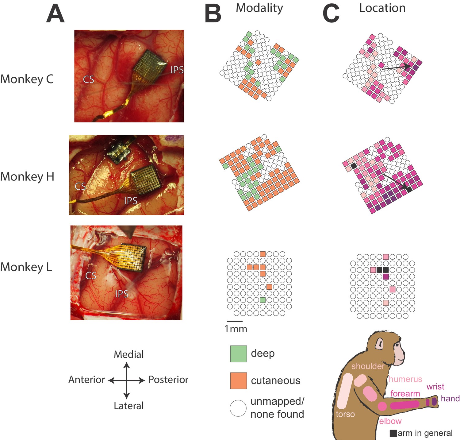
Array locations and receptive field maps from one mapping session for each monkey.
(A) Locations of Utah arrays implanted in area 2 of Monkeys C, H, and L. IPS, intraparietal sulcus; CS central sulcus. (B) Map of the receptive field modality (deep or cutaneous) for each electrode. (C) Map of receptive field location (see legend on bottom right). Open circles indicate both untested electrodes and tested electrodes with no receptive field found. Black arrows on maps in C show significant gradient across array of proximal to distal receptive fields (see Materials and methods).
Figure 2
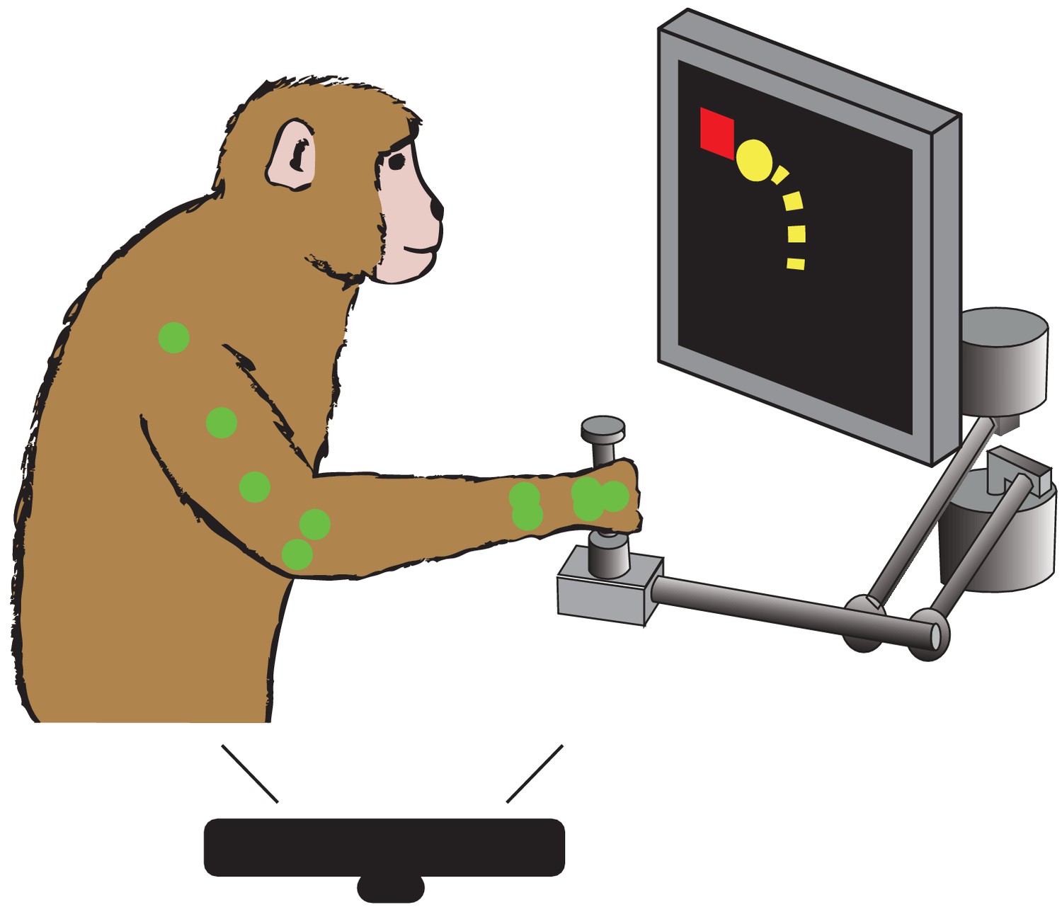
Behavioral task.
Monkey controls a cursor on screen (yellow) with a two link manipulandum to reach to visually presented targets (red). We track the locations of different colored markers (see Materials and methods) on the monkey’s arm (here shown green) during the task, using a Microsoft Kinect.
Figure 3
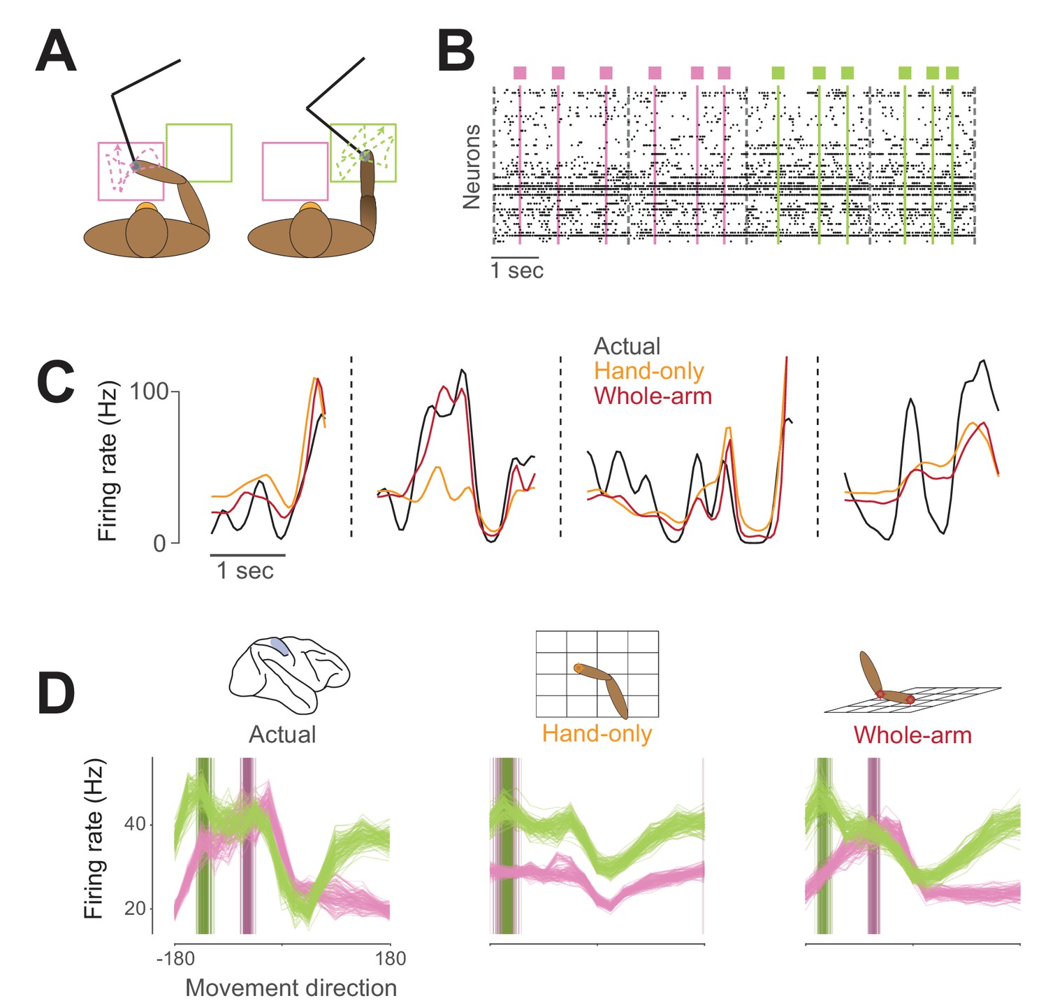
Example neural activity for two-workspace task.
(A) Two-workspace behavior. On each trial, monkey reaches with manipulandum (black) to randomly placed targets in one of two workspaces: one close to the body and contralateral to the reaching hand (pink) and the other distant and ipsilateral (green). Trials in the two workspaces were interleaved randomly. (B) Example neural raster plot from one session for two randomly drawn trials in each workspace. Dots in each row represent activity for one of the simultaneously recorded neurons. Black dashed lines indicate starts and ends of trials, and colored lines and boxes indicate times of target presentation, with color indicating the workspace for the trial. (C) Firing rate plot for an example neuron during four randomly drawn trials from the distal (green) workspace. Black trace represents neural firing rate, smoothed with a 50 ms Gaussian kernel. Colored traces represent unsmoothed firing rates predicted by hand-only (orange), and whole-arm (red) models. (D) Actual and predicted tuning curves and preferred directions (PDs) computed in the two workspaces for an example neuron. Each trace represents the tuning curve or PD calculated for one cross-validation fold (see Materials and methods). Leftmost plot shows actual tuning curves and PDs, while other plots show curves and PDs for activity predicted by each of the models. Each panel shows mean movement-related firing rate plotted against direction of hand movement for both workspaces. Darker vertical bars indicate preferred directions.
Figure 4
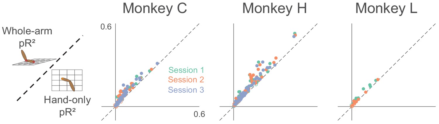
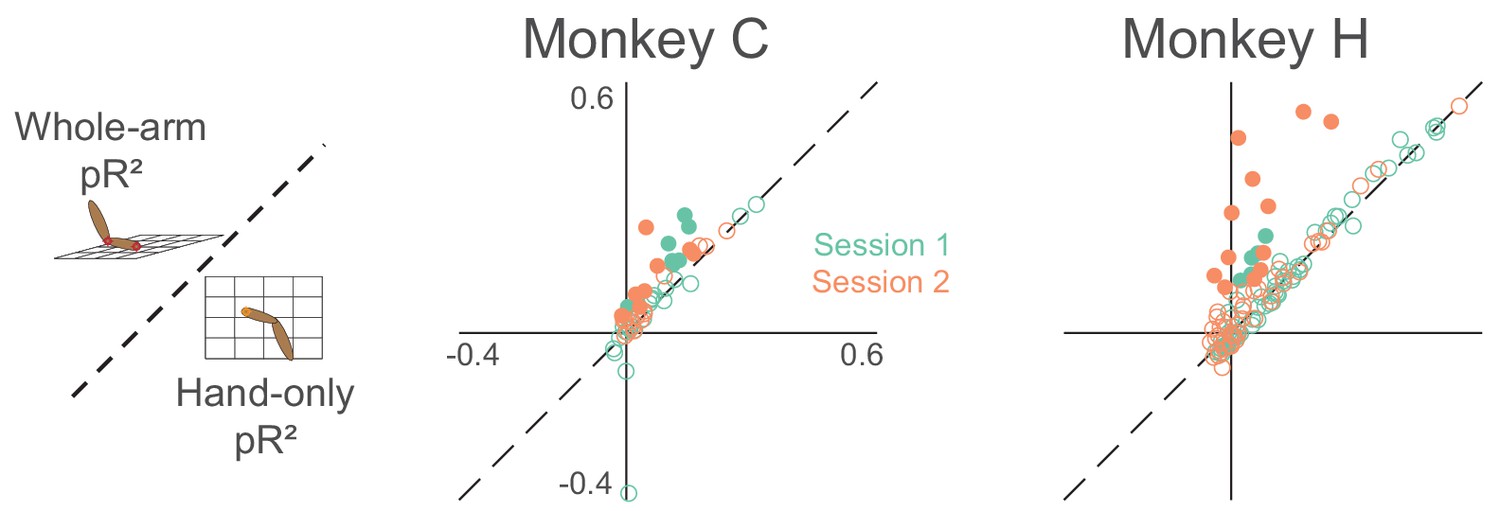
Goodness-of-fit comparison analysis.
Scatter plots compare the pseudo-R2 (pR2) of the whole-arm model to that of the hand-only model for each monkey. Each point in the scatter plot represents the pR2 values of one neuron, with whole-arm pR2 on the vertical axis and hand-only pR2 on the horizontal. Different colors represent neurons recorded during different sessions. Filled circles represent neurons for which one model’s pR2 was significantly higher than that of the other model. In this comparison, all filled circles lie above the dashed unity line, indicating that the whole-arm model performed better than the hand-only model for every neuron in which there was a significant difference.
Figure 5
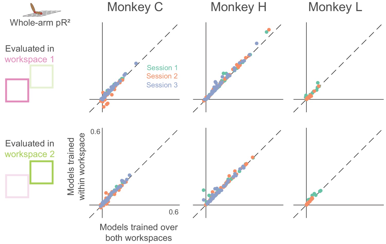
Dependence of whole-arm model accuracy on workspace location of training data.
Each panel compares a model trained and tested in the same workspace (either near or far) to a model trained on data from both workspaces. Each dot corresponds to a single neuron, where color indicates the recording session. Dashed line is the unity line.
Figure 6

Tuning curve shape correlation analysis.
Scatter plot compares tuning curve shape correlation between whole-arm and hand-only models. Filled circles indicate neurons significantly above or below the dashed unity line. As for pR2, most filled circles lie above the dashed line of unity, indicating that the whole-arm model was better at predicting tuning curve shape than the hand-only model.
Figure 7
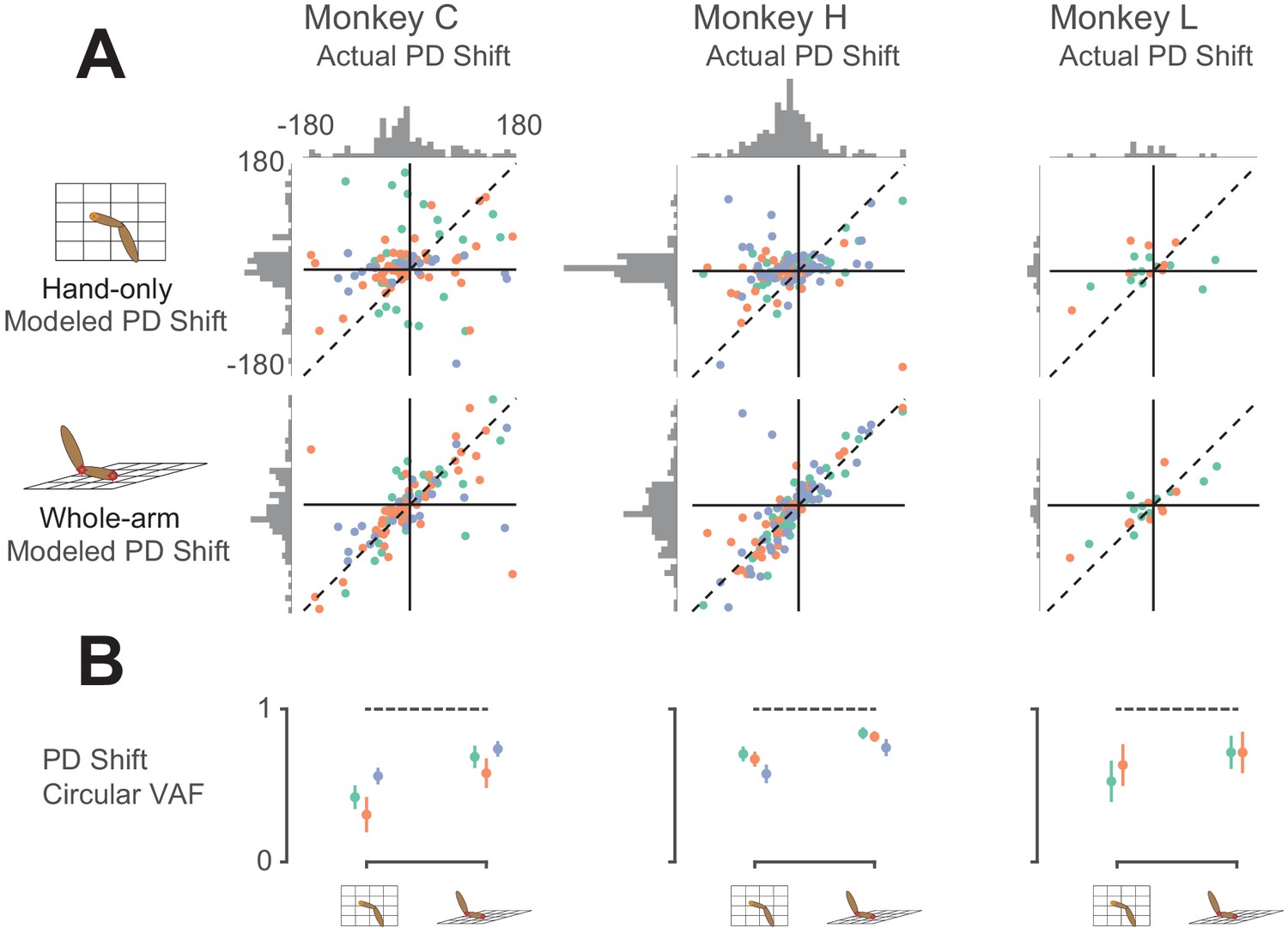
Model predictions of PD shift.
(A) Scatter plots of model-predicted PD shifts plotted against actual PD shifts. Each dot represents the actual and modeled PD shifts of a single neuron, where different colors correspond to neurons recorded during different sessions. Dashed diagonal line shows perfect prediction. Horizontal histograms indicate distributions of actual PD shifts for each monkey. Vertical histograms indicate distributions of modeled shifts. Note that both horizontal and vertical axes are circular, meaning that opposing edges of the plots (top/bottom, left/right) are the same. Horizontal histograms show that the distribution of actual PD shifts included both clockwise and counter-clockwise shifts. Clustering of scatter plot points on the diagonal line for the whole-arm model indicates that it was more predictive of PD shift. (B) Plot showing circular VAF (cVAF) of scatter plots in A, an indicator of how well clustered points are around the diagonal line (see Materials and methods for details). Each point corresponds to the average cVAF for a model in a given session (indicated by color), and the horizontal dashed lines indicate the cVAF for perfect prediction. Error bars show 95% confidence intervals (derived from cross-validation – see Materials and methods). Pairwise comparisons between model cVAFs showed that the whole-arm model out-performed the hand-only model in all but one session, in which the two models were not significantly different.
Figure 8
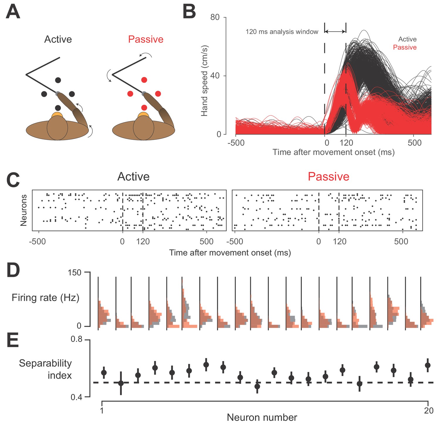
Active vs.passive behavior.
(A) Schematic of task. On active trials (black), monkey reaches from center target to a target presented in one of four directions, indicated by the black circles. On passive trials, manipulandum bumps monkey’s hand in one of the four target directions (red circles). (B) Speed of hand during active (black) and passive (red) trials, plotted against time, for one session. Starting around 120 ms after movement onset, a bimodal distribution in passive movement speed emerges. This bimodality reflects differences in the impedance of the arm for different directions of movement. Perturbations towards and away from the body tended to result in a shorter overall movement than those to the left or right. However, average movement speed was similar between active and passive trials in this 120 ms window, which we used for data analysis. (C) Neural raster plots for example active and passive trials for rightward movements. In each plot, rows indicate spikes recorded from different neurons, plotted against time. Vertical dashed lines delimit the analysis window. (D) Histograms of firing rates during active (black) and passive (red) movements for 20 example neurons from one session with Monkey H. (E) Separability index for each neuron during the session, found by testing how well linear discriminant analysis (LDA) could predict movement type from the neuron’s average firing rate on a given trial. Black dashed line indicates chance level separability. Error bars indicate 95% confidence interval of separability index.
Figure 9
Goodness-of-fit comparison analysis for active/passive experiment (same format as Figure 4).
Each dot represents a single neuron, with color indicating the recording session. Filled circles indicate neurons that are significantly far away from the dashed unity line.
Figure 10
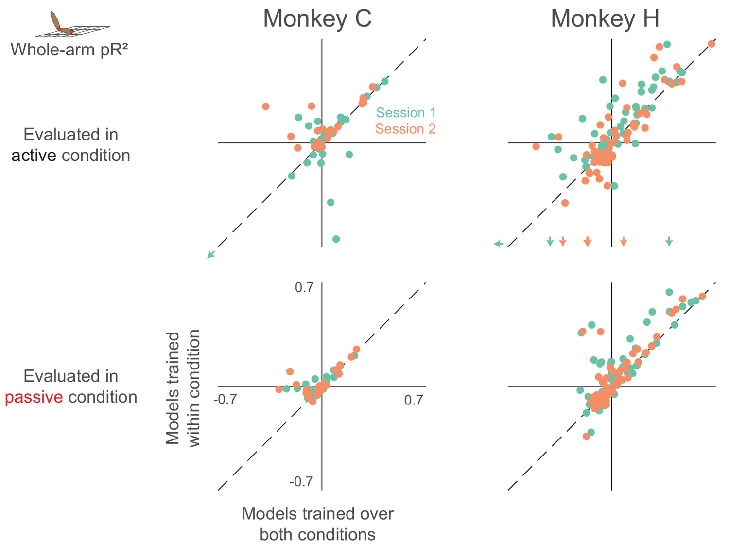
Dependence of whole-arm model accuracy on active and passive training data (same format as Figure 5).
Plots in the upper row contain colored arrows at the edges indicating neurons with pR2 value beyond the axis range, which we omitted for clarity.
Figure 11
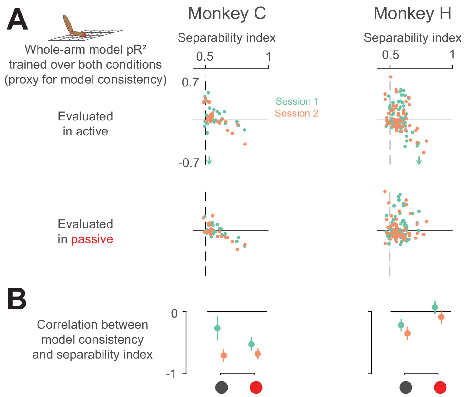
Neural separability index predicts whole-arm model inconsistency.
(A) Scatter plots comparing the consistency of the whole-arm model against the separability index. Conventions are the same as in Figure 10. (B) Correlation between model consistency and separability index. Each dot represents the correlation between model consistency and separability index for a given session, with error bars representing the 95% confidence intervals.
Appendix 1—figure 1
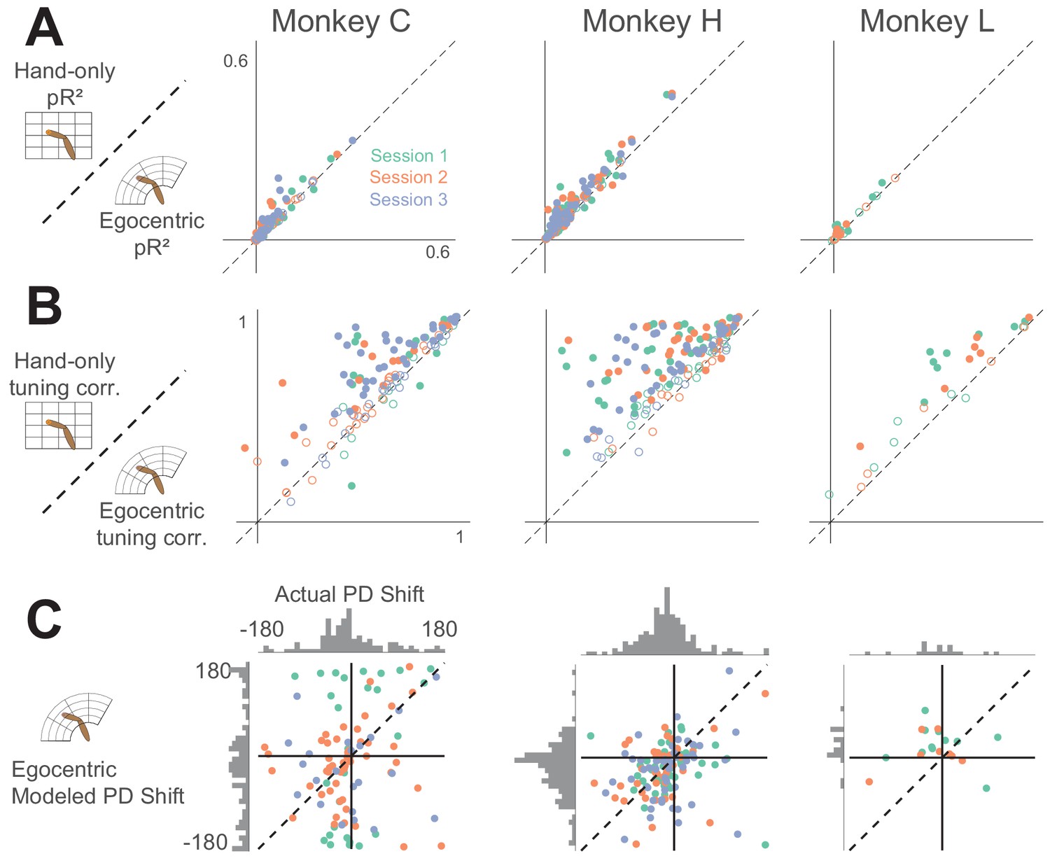
Comparison between hand-only model and egocentric model.
Appendix 1—figure 2
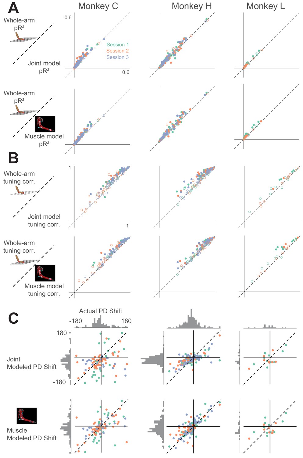
Comparison between whole-arm model and biomechanical models (joint kinematics and musculotendon length).
Same arrangement as in Appendix 1—figure 1.
Appendix 1—figure 3
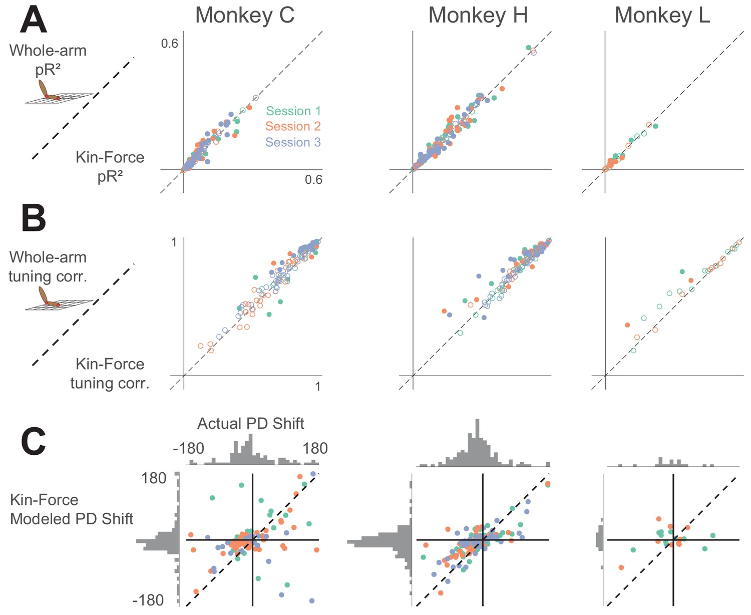
Comparison between whole-arm model and hand kinematic-force model (shortened as ‘Kin-Force’).
Same format as Appendix 1—figures 1 and 2.
Tables
Key resources table
| Reagent type (species) or resource | Designation | Source or reference | Identifiers | Additional information |
|---|---|---|---|---|
| Software, algorithm | MATLAB | MathWorks | RRID: SCR_001622 | All code developed for this paper available on GitHub (See relevant sections of Materials and methods) |
Additional files
Download links
A two-part list of links to download the article, or parts of the article, in various formats.
Downloads (link to download the article as PDF)
Open citations (links to open the citations from this article in various online reference manager services)
Cite this article (links to download the citations from this article in formats compatible with various reference manager tools)
Area 2 of primary somatosensory cortex encodes kinematics of the whole arm
eLife 9:e48198.
https://doi.org/10.7554/eLife.48198


