The perception and misperception of optical defocus, shading, and shape
- The University of Sydney, Australia
Figures
Figure 1
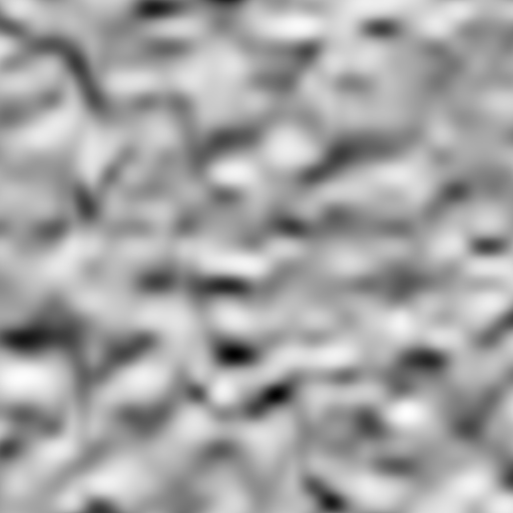
A deformed matte terrain illuminated by a light source elevated 45° above the line of sight.
Despite being rendered in full focus, the image appears blurry, and the local features of its 3D shape seem difficult to perceive.
Figure 2 with 2 supplements
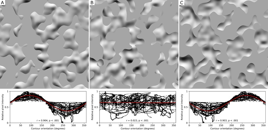
Orientation-intensity covariation induced by level cut contours.
(A) The same shaded surface as shown in Figure 1, but now partially occluded by a gray level cut mask. The mask’s contours were created by intersecting the deformed terrain with a flat plane, and completely eliminate the percepts of blur experienced in Figure 1. The plot beneath reveals how image intensity at the contour varies as an approximate cosine function of orientation. Every pixel of shading along the contour is represented in this plot as a black dot. The correlation coefficient of the cosine fit and its p-value are shown within the graph. (B) The level cut mask that occludes the gradients in (A) has been rotated by 180 degrees over the image, which eliminates the relationship between the contours and surface geometry. The plot below the image reveals the destructive effect of this rotation on the systematic covariation between contour orientation and image intensity. Here, the shading gradients are misperceived as either a flat texture or a blurred surface beneath a floating stencil. (C) The contours shown in (A) now form a mask that occludes every part of the shaded surface in front of the level cut. The orientation-intensity covariation along the contour is equally strong, but the 180° shift in its phase causes the gradients to appear bistable: either bumps lit from below, or concavities lit from above. These gradients appear less focused overall than the unambiguously convex surface in (A).
Figure 2—figure supplement 1
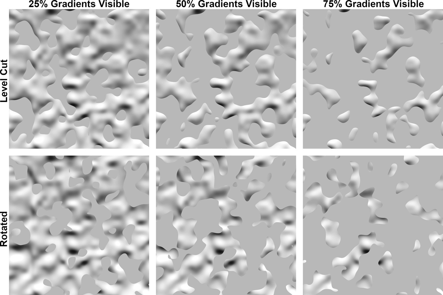
The ‘convex’ level cut (top) and rotated (bottom) mask conditions used in Experiment 1.
The masks in the top row exclude all surface regions at a greater depth than the level cut contours, and the remaining visible gradients appear vividly convex. These masks have been rotated by 180° in the bottom row, which destroys the geometric relationship between the contours and the 3D surface. The percentage of visible gradients increases with the depth of the level cut from left to right. The top-center image is also shown in Figure 2A.
Figure 2—figure supplement 2
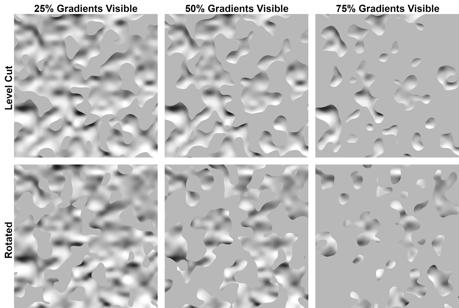
The ‘bistable’ level cut (top) and rotated (bottom) mask conditions used in Experiment 1.
The level cut contours of the masks in the top row are identical to those in the top row of Figure 2—figure supplement 1, but the masks now exclude all surface regions at a nearer depth than the level cut contours. The visible gradients are bistable: they can appear as concave dents illuminated from above or convex bumps illuminated from below (or neither). The bottom row depicts rotated versions of these masks that are no longer related to surface geometry. Note that the depth of the level cut now decreases from left to right to produce images with a greater percentage of visible gradients. The top-center image is also shown in Figure 2C.
Figure 3
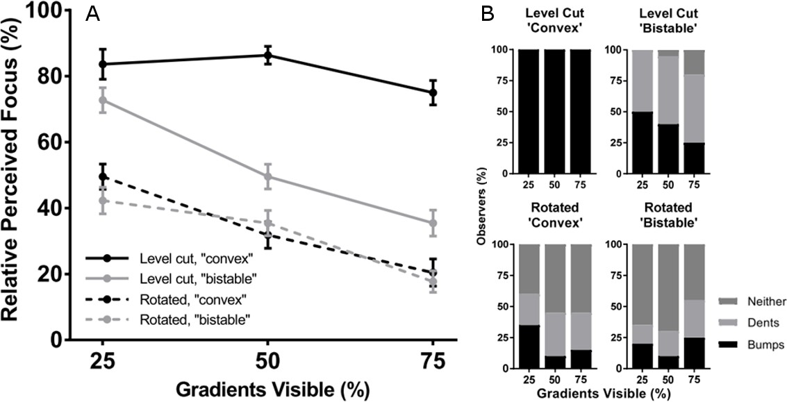
Perceived focus and shape in Experiment 1.
(A) Perceived focus in Experiment 1. The horizontal axis represents the percentage of gradients visible and the four lines represent the four combinations of mask rotation (level cut vs. rotated) and mask occlusion style (‘convex’ vs. ‘bistable’). The vertical axis represents the percentage of trials in which each stimulus was chosen as appearing most focused. Error bars represent ± 1 S.E.M. (B) Perceived curvature type in Experiment 1. In each stacked column plot, the horizontal axis represents the percentage of visible gradients and the vertical axis represents the percentages of observers who perceived that stimulus as convex bumps (black), concave dents (light gray), or neither (dark gray). Each plot depicts a different combination of mask rotation (level cut vs. rotated) and mask occlusion style (‘convex’ vs. ‘bistable’). The observers were the same group as in (A).
Figure 4
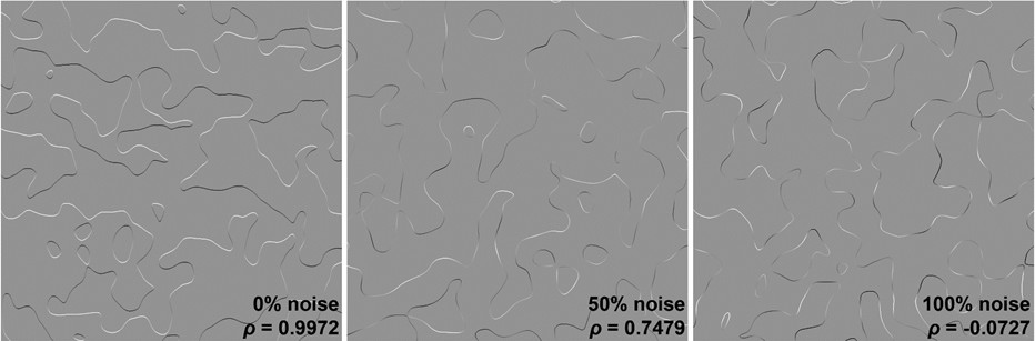
Example stimuli used in Experiment 2.
The stimuli were created by mixing varying amounts of random noise with shaded ribbons designed to exhibit a perfect linear correlation between orientation (relative to 90°) and intensity. The examples shown here increase in noise from left to right. The computed global correlations between relative ribbon orientation and intensity are shown in the bottom-right of each stimulus.
Figure 5

Perceived 3D shape in Experiment 2.
The horizontal axes represent the percentage of gradient noise in the shaded ribbons (left) and bins of computed Pearson correlation coefficients between ribbon orientation and shading intensity (right). The rightmost bin in the right panel contains all correlation coefficients below 0.4, and all other bins have a width of 0.1. The vertical axis in each plot represents the percentage of trials in which each condition (left) or correlation value (right) was chosen as appearing most vividly 3D out of the total number of trials in which that condition or correlation value appeared. Error bars represent ± 1 S.E.M.
Figure 6
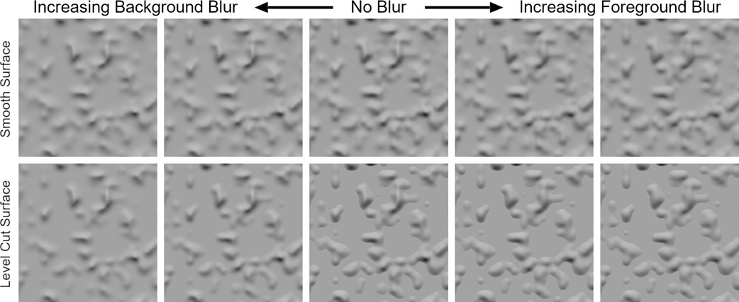
Stimuli used in Experiment 3.
The top row depicts the ‘smoothed’ surface with no intersecting plane and the bottom row depicts the ‘level cut’ surface with the intersecting plane. From left to right, the columns depict the strong background blur, weak background blur, no blur, weak foreground blur, and strong foreground blur conditions.
Figure 7
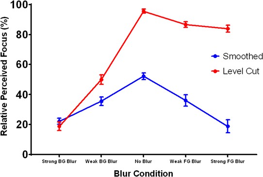
Perceived focus in Experiment 3.
The horizontal axis represents the five blur conditions and the vertical axis represents the percentage of trials in which each stimulus was chosen as appearing most focused. The blue and red lines depict the results for the smoothed and level cut surfaces, respectively. Error bars represent ± 1 S.E.M.
Figure 8
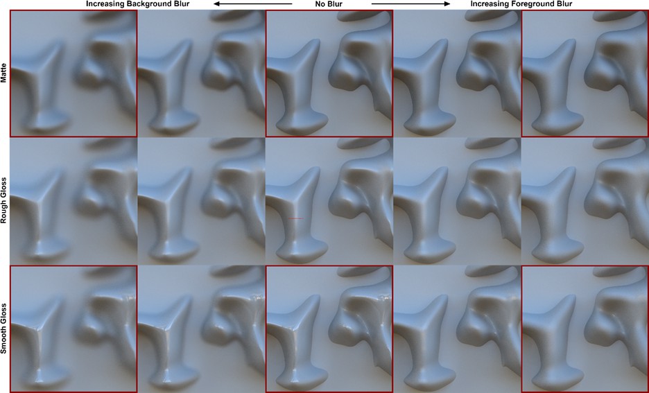
Stimuli used in Experiment 4.
From top to bottom, the rows depict the surfaces with matte reflectance, rough gloss, and smooth gloss. From left to right, the columns depict the conditions with strong background (BG) blur, weak background blur, no blur, weak foreground (FG) blur, and strong foreground blur. Perceived focus and gloss were measured for all fifteen stimuli. Perceived 3D shape was measured horizontally across the prominent vertical ridge in the six stimuli outlined in red. The probe points where shape measurements were taken are shown as red dots in the central stimulus.
Figure 9

Perceived focus in Experiment 4.
The horizontal axis represents the five blur conditions and each colored line represents a different reflectance condition. The vertical axis represents the percentage of trials in which each stimulus was selected as appearing most focused. Error bars represent ± 1 S.E.M.
Figure 10
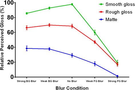
Perceived gloss in Experiment 4.
The horizontal axis represents the five blur conditions and each colored line represents a different reflectance condition. The vertical axis represents the percentage of trials in which each stimulus was selected as appearing most glossy. Error bars represent ± 1 S.E.M.
Figure 11

Average shape profiles reconstructed from measurements of surface orientation in Experiment 4.
The top panel depicts profiles for the matte conditions and the bottom panel depicts profiles for the smooth gloss conditions. The horizontal axis in each plot represents probe location and the vertical axis representsthe height of the contour in normalized units of distance relative to the maximum reconstructed height for each observer. The blue, red, and green lines depict the shape profiles for the strong background (BG) blur, no blur, and strong foreground (FG) blur conditions respectively. Error bars represent ± 1 S.E.M. in normalized units.
Figure 12
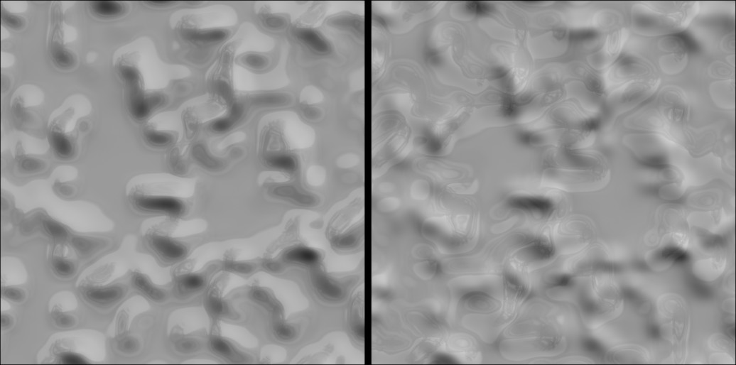
The surface used in Experiment 3 has here been rendered with added specular reflections in a natural light field (left).
In the right panel, the specular reflections have been rotated by 180 degrees relative to the shading gradients, which breaks their apparent attachment to the surface and reduces the perception of both surface gloss and gradient focus.
Additional files
-
Transparent reporting form
- https://doi.org/10.7554/eLife.48214.017
Download links
A two-part list of links to download the article, or parts of the article, in various formats.
Downloads (link to download the article as PDF)
Open citations (links to open the citations from this article in various online reference manager services)
Cite this article (links to download the citations from this article in formats compatible with various reference manager tools)
The perception and misperception of optical defocus, shading, and shape
eLife 8:e48214.
https://doi.org/10.7554/eLife.48214


