Figures and data in Plasticity of cell migration resulting from mechanochemical coupling

Figures
Videos
Tables
Additional files

4 figures, 4 videos, 1 table and 1 additional file

Figures

Figure 1

Download asset Open asset

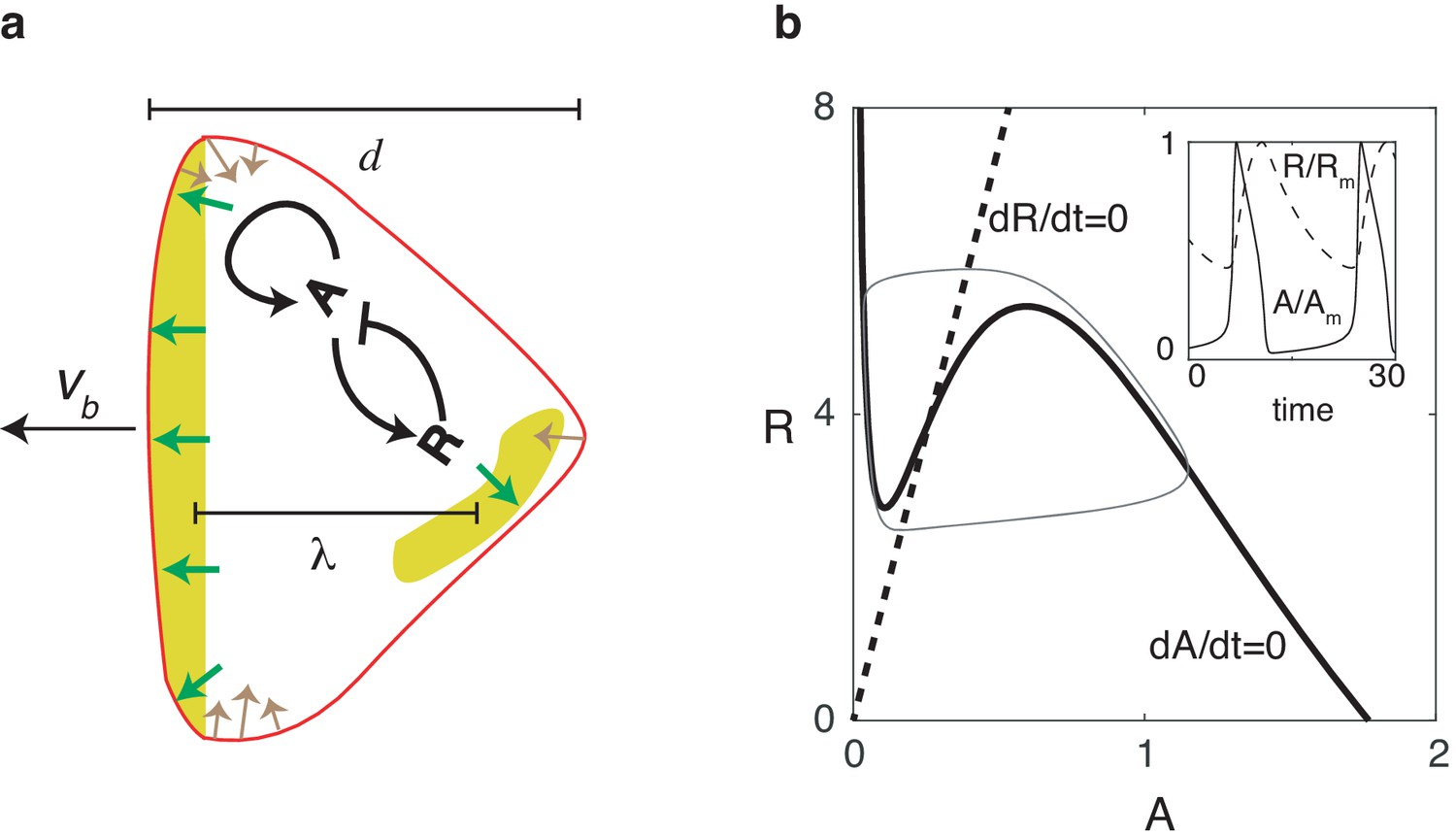
Reaction diffusion model coupled to a mechanical model.

(a) Schematic illustration of the two-dimensional model: a self-activating activator field $A$ , indicated in color, drives the movement of the cell membrane through protrusive forces that are normal to the membrane (green arrows). The membrane tension (denoted by brown arrows) is proportional to the local curvature while the cell also experiences a drag force that is proportional to the speed. One successive wave is generated behind the original one after a distance of $λ$ . The cell’s front-back distance is $d$ , and the cell boundary is pushed outward with speed $v_{b}$ . (b) Nullclines of the activator (solid line) and inhibitor (dashed line), along with the resulting trajectory in phase space (gray thin line). The inset shows the oscillations of $A$ and $R$ , normalized by their maximum values $A_{m}$ and $R_{m}$ .

https://doi.org/10.7554/eLife.48478.002

Figure 2 with 6 supplements

Download asset Open asset

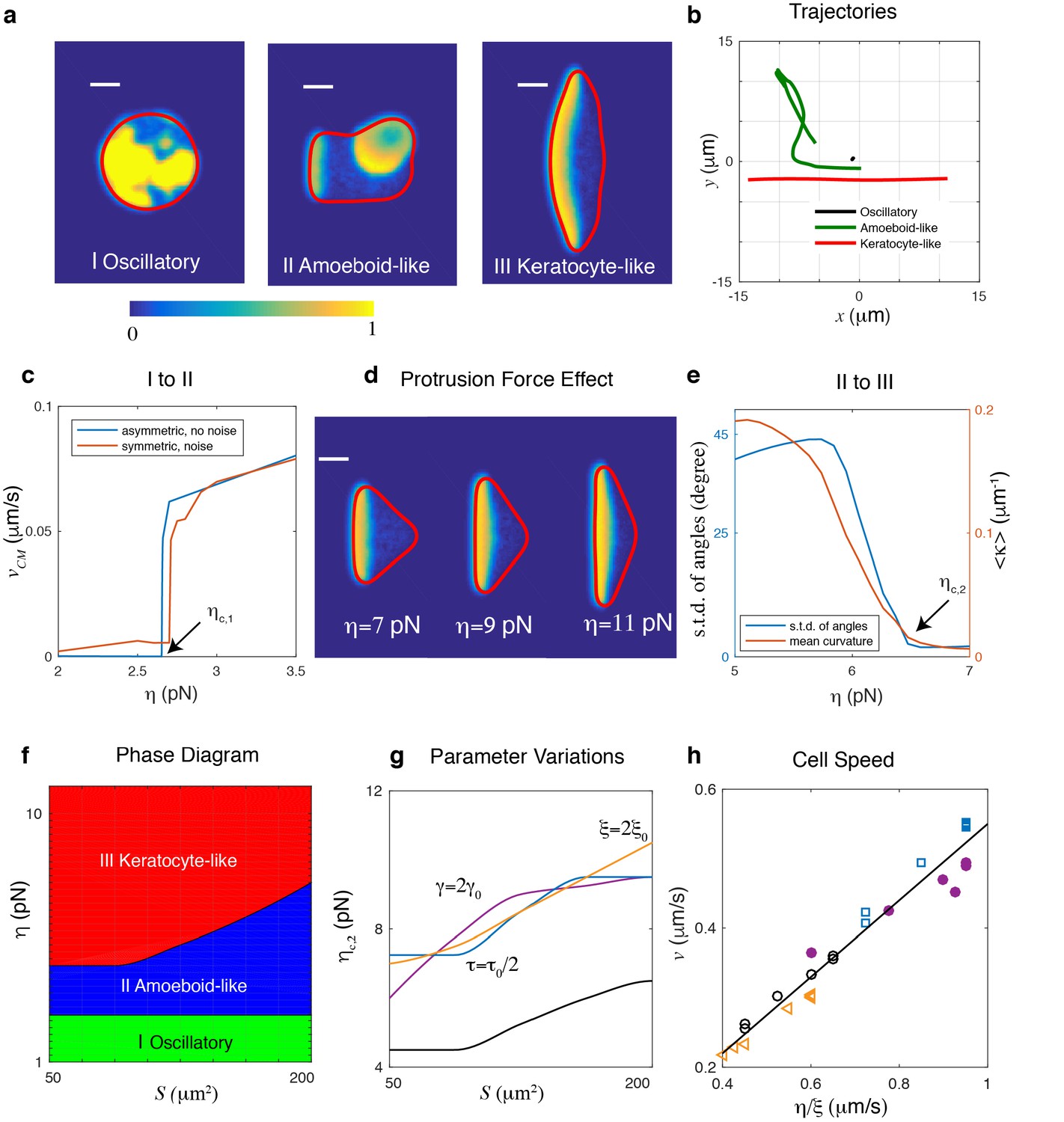
Different cell migration modes can be captured in the model by varying the protrusive strength $η$ .

(a) Snapshots of a simulated cell showing (I) an oscillatory cell ( $η = 2 p N$ ), (II) an amoeboid-like cell ( $η = 4 p N$ ), and (III) a keratocyte-like cell ( $η = 11 p N$ ). All other parameters were assigned the default values and r = 8µm. Here, the activator concentration is shown using the color scale and the cell membrane is plotted as a red line (scale bar µm). (b) The trajectories of the three cells in (a). (c) The transition from oscillatory cell to amoeboid-like cell, with speed of the center of mass of a cell as a function of protrusion strength $η$ for r = 8µm. The red curve represents results from initial conditions where noise is added to a homogeneous $A$ and $R$ field while the blue curve corresponds to simulations in which the initial activator is asymmetric. Cells become non-motile at a critical value of protrusion strength, $η_{c, 1}$ . (d) Increasing the protrusive force $η$ will result in flatter fronts in keratocyte-like cells and a decreased front-back distance. The simulations are carried out for fixed cell area $S$ . (e) The transition from amoeboid-like cell to keratocyte-like cell quantified by either the average curvature along a trajectory or the standard deviation of the angles of trajectory points as a function of protrusion strength $η$ (r = 8µm). Cell moves unidirectionally when the protrusion strength $η > η_{c, 2}$ . (f) Phase diagram determined by systematically varying $η$ and the initial radius of the cell, $r$ . Due to strong area conservation, cell area is determined through $S = π r^{2}$ . (g) The transition line of amoeboid-like cell to keratocyte-like cell for different parameter values. (h) The speed of the keratocyte-like cell as a function of $η / ξ$ . The black line is the predicted cell speed with $v_{b} = α η / ξ$ , where $α \approx 0.55$ . Symbols represent simulations using different parameter variations: empty circles, default parameters; triangles, $ξ = 2 ξ_{0}$ ; filled circles, $γ = 2 γ_{0}$ ; squares, $τ = τ_{0} / 2$ .

https://doi.org/10.7554/eLife.48478.004

Figure 2—figure supplement 1

Download asset Open asset

Speed of keratocyte-like cells as a function of the surface tension and timescale of the inhibitor.

Speed of keratocyte-like cells as a function of the surface tension (a) and the timescale of the inhibitor (b). Parameters are as in Table 1 with r = 8µm.

https://doi.org/10.7554/eLife.48478.005

Figure 2—figure supplement 2

Download asset Open asset

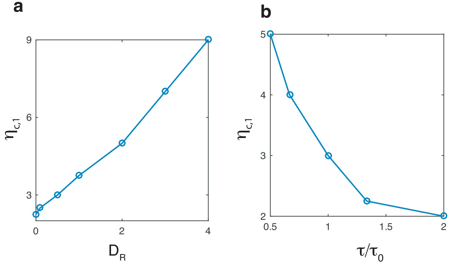
Critical protrustion strength $η_{c, 1}$ as a function of the inhibitor’s diffusion constant and time scale.

(a) The critical value $η_{c, 1}$ of protrusion strength as a function of inhibitor’s diffusion constant $D_{R}$ , and (b), the timescale of the inhibitor $τ$ , rescaled by the default value $τ_{0} = 10 s$ . Remaining parameters are as in Table 1 with r = 8µm.

https://doi.org/10.7554/eLife.48478.006

Figure 2—figure supplement 3

Download asset Open asset

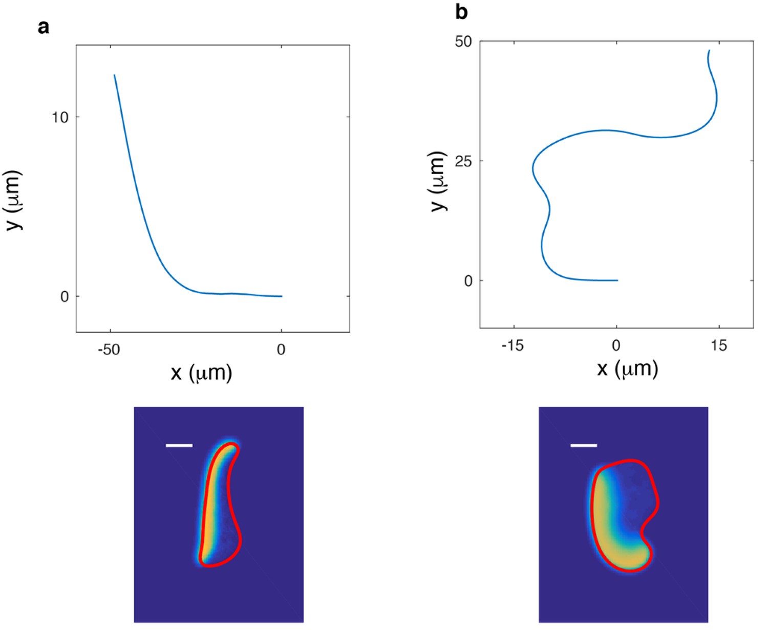
Effects of tension.

Snapshot (bottom) and corresponding trajectory (top) of a cell that undergoes a turning instability. (a) Upon the reduction of surface tension from $γ$ =2pN/µm to $γ$ =1pN/µm. Parameters are taken from Table 1 with r = 6µm. (b) As in (a), but now after an increase in $D_{A}$ and $D_{R}$ to $D_{A} = D_{R}$ =2 µm²/s and r = 8µm.

https://doi.org/10.7554/eLife.48478.007

Figure 2—figure supplement 4

Download asset Open asset

Parameter variations in the model.

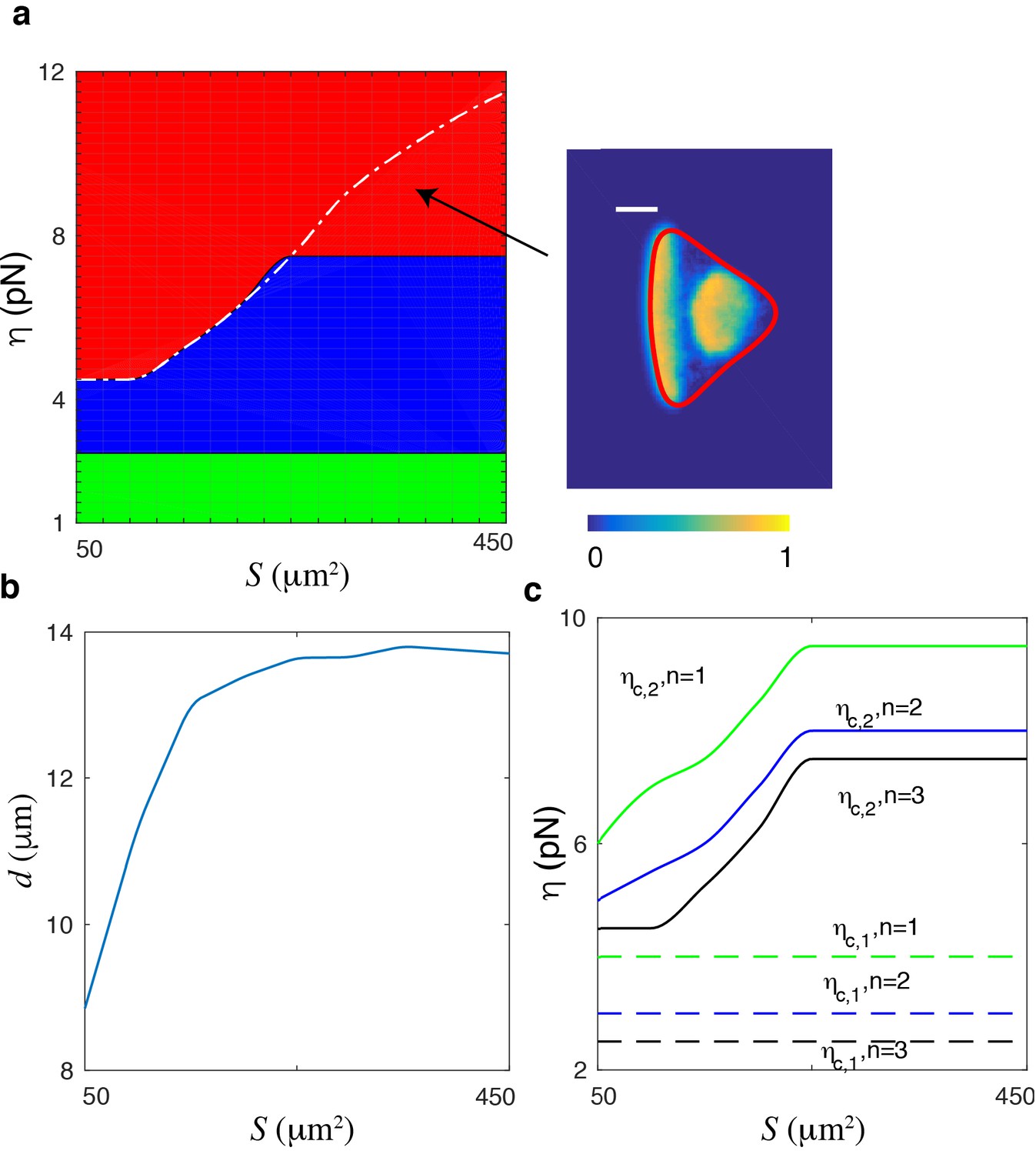
Parameter variations in the model. (a) Phase space extended to maximum cell area ~ 450 µm², corresponding to r = 12µm. Green: oscillatory cell; blue: amoeboid-like cell; red: keratocyte-like cell. The dashed white line corresponding to the separation line $d = λ$ above which the keratocyte-like cells exhibit a single wave and below which keratocyte-like cells move unidirectional but with small waves repeatedly appearing at the back of the cell. (b) The keratocyte-like cell’s front-back distance $d$ along the white dashed line. The saturation value is the wavelength $λ \approx 13 μ m$ . (c) Lines corresponding to $η_{c, 1}$ and $η_{c, 2}$ in the $(η, S)$ phase space for different values of the Hill coefficient $n$ . For all values of $n$ used in the simulations, $η_{c, 1}$ is independent of the cell radius $r$ while $η_{c, 2}$ increases with $r$ , and thus $S$ , and eventually saturates.

https://doi.org/10.7554/eLife.48478.008

Figure 2—figure supplement 5

Download asset Open asset

Oscillatory cells for strong and weak area conservation.

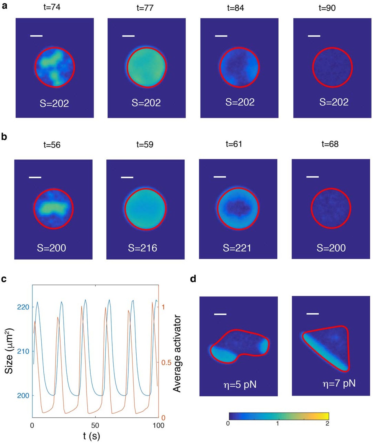
Oscillatory cells for strong (a, $B_{S} = 10$ ) and weak (b, $B_{S} = 0.1$ ) area conservation. Parameters are as in Table 1 with $η = 2.5$ and r = 8µm. (c) Cell size (blue) and average activator concentration (red) as a function of time for the oscillatory cell in panel b. (d) Left, example of amoeboid-like cell for weak area conservation ( $B_{S} = 0.1$ ); right, example of keratocyte-like cell for weak area conservation ( $B_{S} = 0.1$ ). The colors represent the activator concentration, as indicated by the color bar. Scalebar = 5 µm.

https://doi.org/10.7554/eLife.48478.009

Figure 2—figure supplement 6

Download asset Open asset

Excitable dynamics can reproduce identical qualitative results.

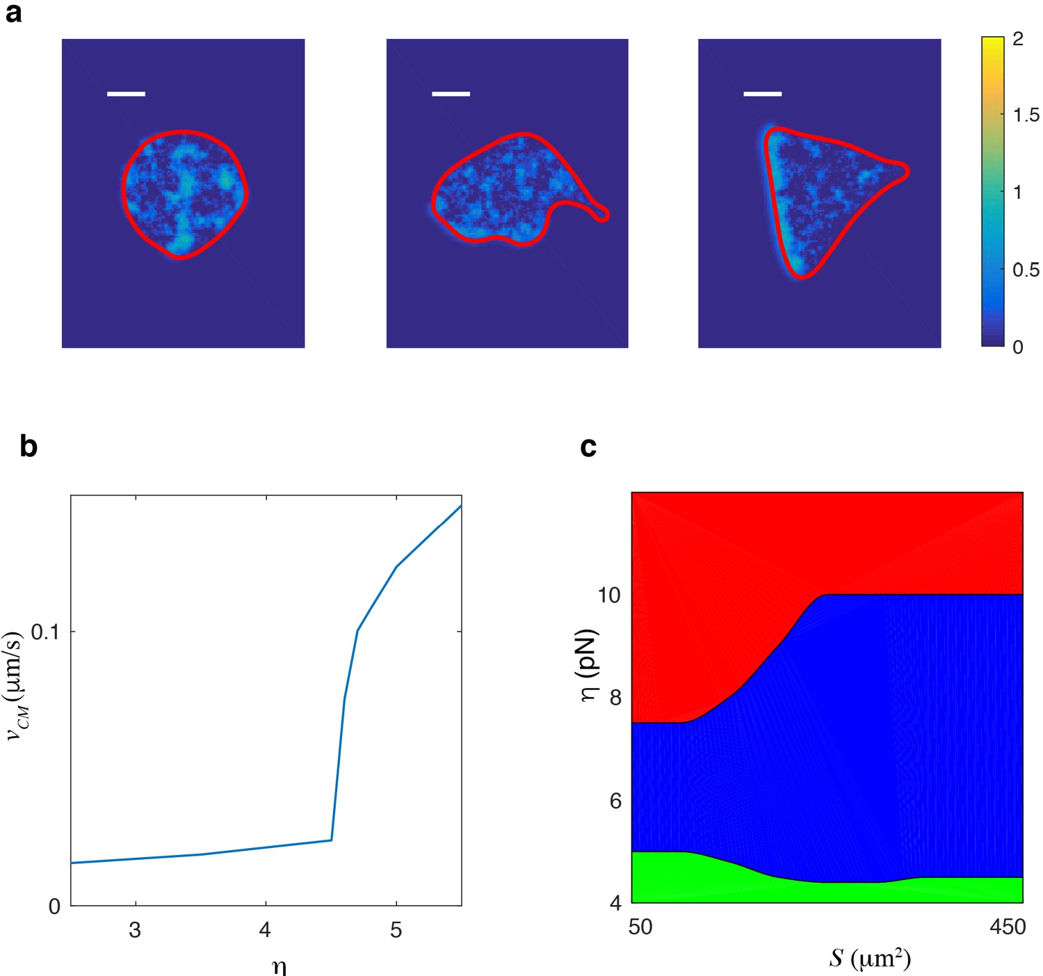
Excitable dynamics can reproduce identical qualitative results. (a) Snapshots of the three different migration modes for an excitable version of the model. Left panel shows an nonmotile cell ( $η = 2$ ), middle panel shows an amoeboid-like cell ( $η = 4$ ), and the right panel displays a keratocyte-like cell ( $η = 10$ ). (b) Speed of the center of mass as a function of critical protrusion strength. As for the relaxation oscillator model (Figure 2c), the bifurcation is subcritical. (c) Phase diagram $(η, S)$ space with green corresponding to nonmotile cells, blue representing amoeboid-like cells, and red corresponding to keratocyte-like cells. Scalebar = 5 µm.

https://doi.org/10.7554/eLife.48478.010

Figure 3 with 2 supplements

Download asset Open asset

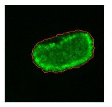
Experiments reveal different migration modes in Dictyostelium cells.

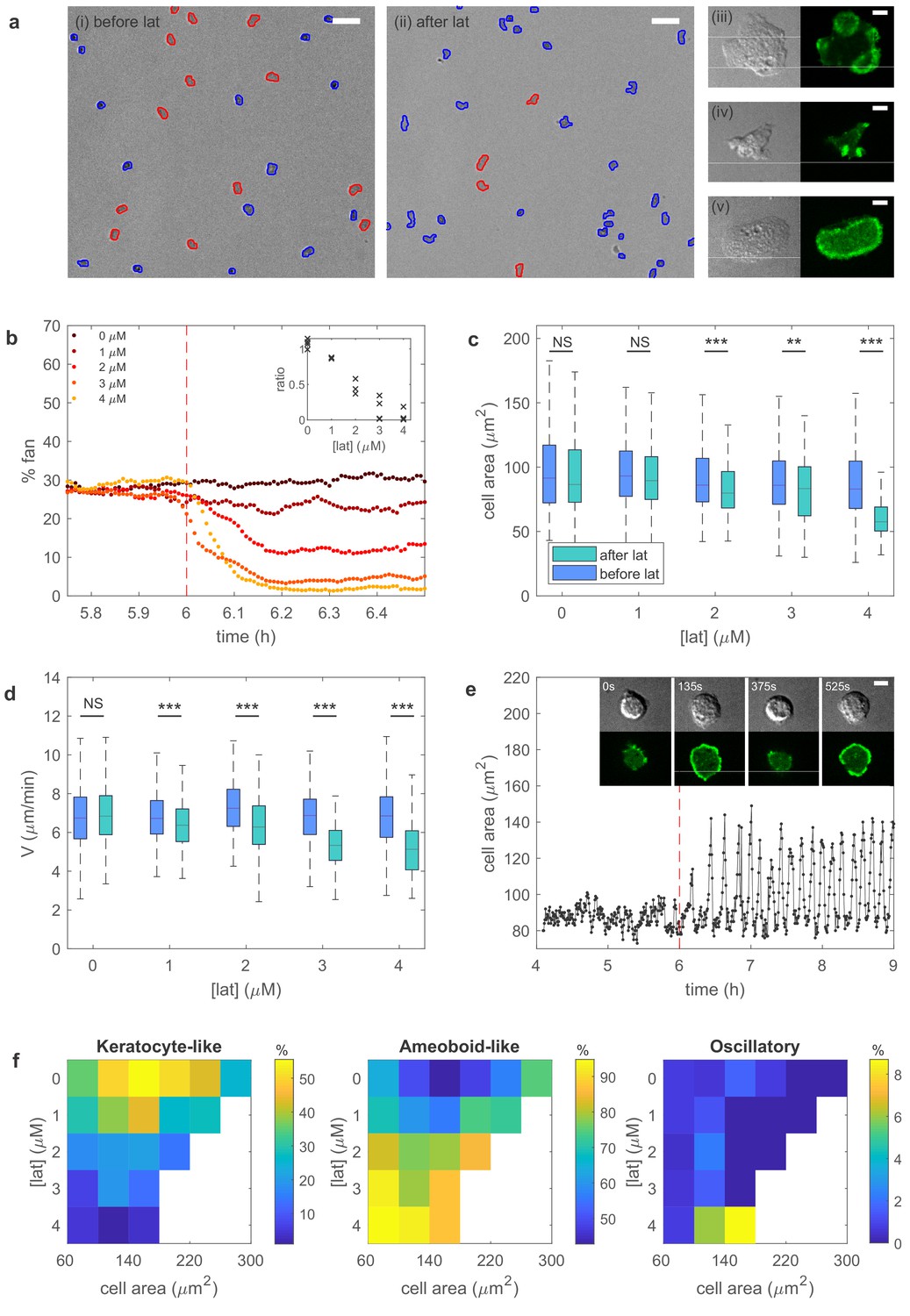
(a) Snapshot of starved Dictyostelium cells before (left) and after (right) exposure to latrunculin B. Amoeboid-like cells are outlined in blue while keratocyte-like cells are outlined in red (scale bar: 50 µm). The panels on the right show high magnification views of amoeboid-like (top two) and keratocyte-like cells in which the freshly polymerized actin is visualized with limE-GFP (scale bar: 5 µm). (b) Percentage of keratocyte-like cells as a function of time for different concentrations of latrunculin B (introduced at 6 hr, dashed line). Inset shows the ratio of keratocyte-like to all cells as a function of the latrunculin concentration for three repeats. (c) The cell area size of keratocyte-like cells before and after latrunculin exposure as a function of concentration. (d) The speed of keratocyte-like cells before and after latrunculin exposure as a function of concentration. (e) Basal cell area as a function of time for a cell that transitioned from amoeboid-like to oscillatory. Insets show snapshots of the cell at different time points (scale bar: 5 µm). (f) Percentage of cells in the keratocyte-like, amoeboid-like, and oscillatory mode of migration in the phase space spanned by cell area and latrunculin concentration. Percentage for each mode is visualized using the color bars. The number of cells for each data point varies between 7 and >1000 and white corresponds to a data point with fewer than seven total cells.

https://doi.org/10.7554/eLife.48478.015

Figure 3—figure supplement 1

Download asset Open asset

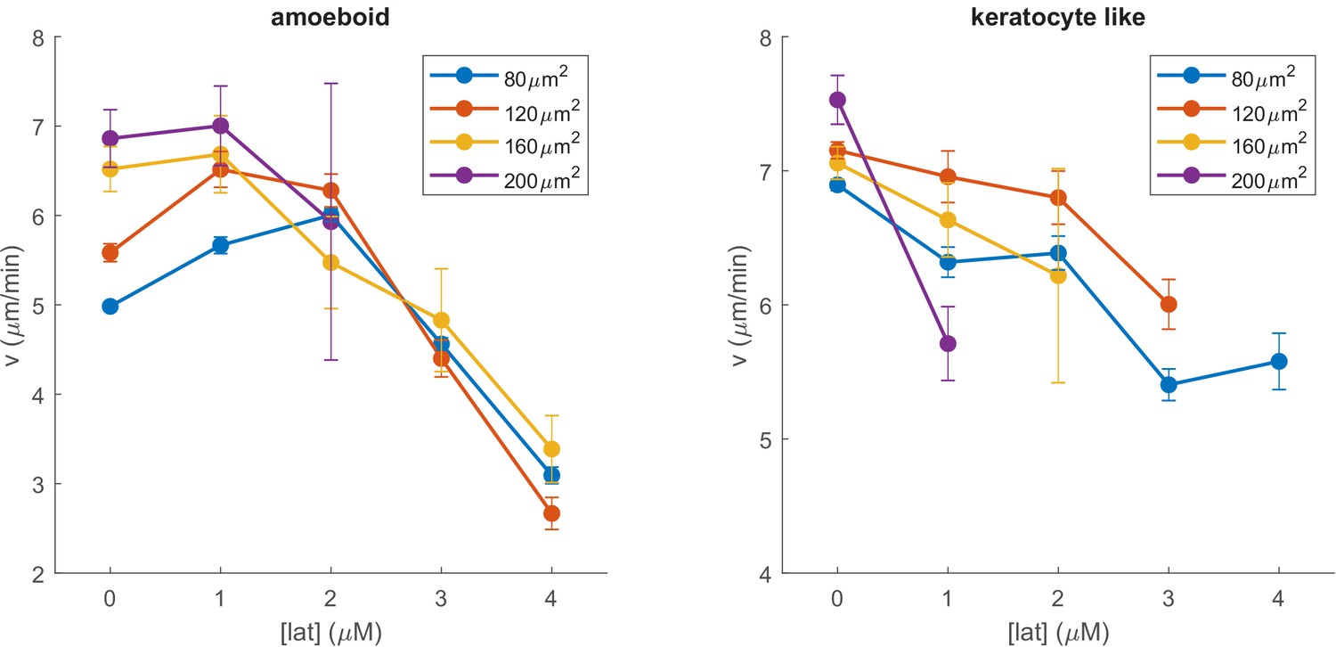
The speed of amoeboid and keratocyte-like cells as a function of latrunculin concentration for different cell areas.

Cell speed decreases as the latrunculin concentration increases. Cell areas were grouped in bins of 40 µm₂. Error bars represent the standard error of the mean.

https://doi.org/10.7554/eLife.48478.016

Figure 3—figure supplement 2

Download asset Open asset

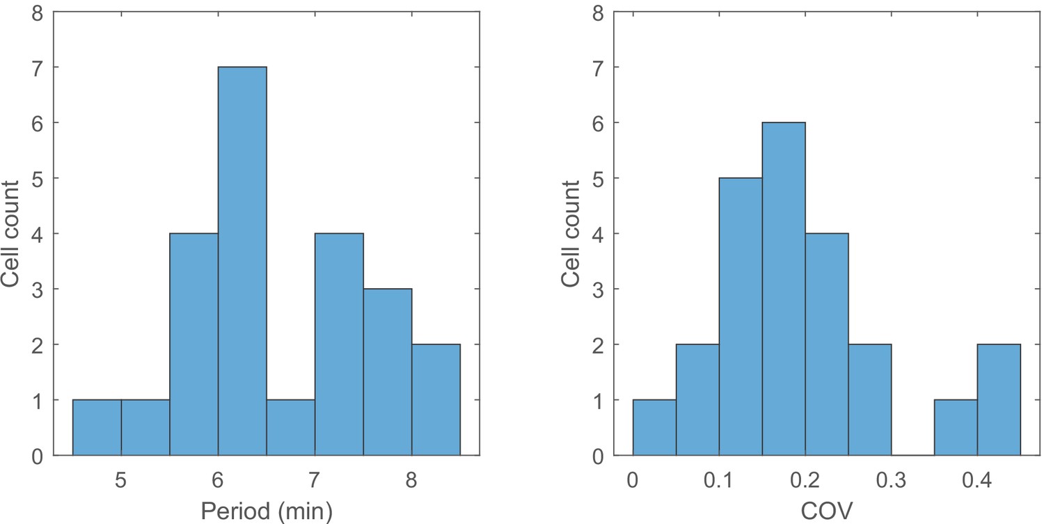
The average period and coefficient of variation for area oscillations in oscillating cells after the exposure to latrunculin.

The average period and coefficient of variation COV (ratio of the standard deviation and the mean) for area oscillations in oscillating cells after the exposure to 4µM latrunculin (N = 23).

https://doi.org/10.7554/eLife.48478.017

Author response image 1

Download asset Open asset

Videos

Video 1

Download asset

posterframe for video — Simulation results for r = 8µm and $η = 2 p N$ . Here, and in all other simulation videos, the activator concentration is shown using a color scale (see Figures).
https://doi.org/10.7554/eLife.48478.011

Video 2

Download asset

Video 3

Download asset

Video 4

Download asset

Tables

Table 1

Model Parameters.

https://doi.org/10.7554/eLife.48478.003

Parameter	Description	Value
$γ$	Tension	2 pN µm
$ϵ$	Width of phase field	2 µm
$B_{S}$	Cell area conservation strength	10 pN/µm²
$ξ$	Friction coefficient	10 pN s/µm²
$n$	Hill coefficient of protrusive force	3
$k_{a}$	Activation rate	10 s^-1
$K_{a}$	Activation threshold	1 µM
$b$	Basal activation rate	0.1 s^-1
$A_{t}$	Total activator concentration	2 µM
$d_{1}$	Basal degradation rate	1 s^-1
$d_{2}$	Degradation rate from inhibitor	1 µM^-1s^-1
$c_{1}$	Inhibitor degradation coeffecient	1
$c_{2}$	Inhibitor activation coefficient	15
$τ$	Time scale of negative feedback	10 s
$D_{A}$	Activator diffusion coefficient	0.5 µm²/s
$D_{R}$	Inhibitor diffusion coefficient	0.5 µm²/s
$σ$	Noise intensity	0.01 µM²/µm²/s
$Δ t$	Time step	0.001 s
$n, m$	Space grid size	256,256
$L_{x, y}$	Space size	50,50 µm

Additional files

Transparent reporting form: https://doi.org/10.7554/eLife.48478.018
Download elife-48478-transrepform-v1.docx

Download links

A two-part list of links to download the article, or parts of the article, in various formats.

Downloads (link to download the article as PDF)

Open citations (links to open the citations from this article in various online reference manager services)

Mendeley

Cite this article (links to download the citations from this article in formats compatible with various reference manager tools)

Yuansheng Cao
Elisabeth Ghabache
Wouter-Jan Rappel

(2019)

Plasticity of cell migration resulting from mechanochemical coupling

eLife 8:e48478.

https://doi.org/10.7554/eLife.48478

Figures

Reaction diffusion model coupled to a mechanical model.

Different cell migration modes can be captured in the model by varying the protrusive strength $η$ .

Speed of keratocyte-like cells as a function of the surface tension and timescale of the inhibitor.

Critical protrustion strength $η_{c, 1}$ as a function of the inhibitor’s diffusion constant and time scale.

Effects of tension.

Parameter variations in the model.

Oscillatory cells for strong and weak area conservation.

Excitable dynamics can reproduce identical qualitative results.

Experiments reveal different migration modes in Dictyostelium cells.

The speed of amoeboid and keratocyte-like cells as a function of latrunculin concentration for different cell areas.

The average period and coefficient of variation for area oscillations in oscillating cells after the exposure to latrunculin.

Videos

Simulation results for r = 8µm and $η = 2 p N$ . Here, and in all other simulation videos, the activator concentration is shown using a color scale (see Figures).

Simulation results for r = 8µm and $η = 4 p N$ .

Simulation results for r = 8µm and $η = 11 p N$ .

Experimental results with 2µM Latrunculin B added at time 1h45min.

Tables

Model Parameters.

Additional files

Transparent reporting form

Download links

Downloads (link to download the article as PDF)

Open citations (links to open the citations from this article in various online reference manager services)

Cite this article (links to download the citations from this article in formats compatible with various reference manager tools)

Be the first to read new articles from eLife

Share this article

Cite this article

Reaction diffusion model coupled to a mechanical model.

Different cell migration modes can be captured in the model by varying the protrusive strength η.

Speed of keratocyte-like cells as a function of the surface tension and timescale of the inhibitor.

Critical protrustion strength ηc,1 as a function of the inhibitor’s diffusion constant and time scale.

Effects of tension.

Parameter variations in the model.

Oscillatory cells for strong and weak area conservation.

Excitable dynamics can reproduce identical qualitative results.

Experiments reveal different migration modes in Dictyostelium cells.

The speed of amoeboid and keratocyte-like cells as a function of latrunculin concentration for different cell areas.

The average period and coefficient of variation for area oscillations in oscillating cells after the exposure to latrunculin.

Simulation results for r = 8µm and η=2pN. Here, and in all other simulation videos, the activator concentration is shown using a color scale (see Figures).

Simulation results for r = 8µm and η=4pN.

Simulation results for r = 8µm and η=11pN.

Experimental results with 2µM Latrunculin B added at time 1h45min.

Model Parameters.

Transparent reporting form

Downloads (link to download the article as PDF)

Open citations (links to open the citations from this article in various online reference manager services)

Cite this article (links to download the citations from this article in formats compatible with various reference manager tools)

Different cell migration modes can be captured in the model by varying the protrusive strength $η$ .

Critical protrustion strength $η_{c, 1}$ as a function of the inhibitor’s diffusion constant and time scale.

Simulation results for r = 8µm and $η = 2 p N$ . Here, and in all other simulation videos, the activator concentration is shown using a color scale (see Figures).

Simulation results for r = 8µm and $η = 4 p N$ .

Simulation results for r = 8µm and $η = 11 p N$ .