Ten simple rules for the computational modeling of behavioral data
- University of Arizona, United States
- University of California, Berkeley, United States
Figures
Figure 1
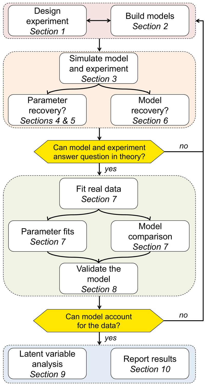
Schematic of the 10 rules and how they translate into a process for using computational modeling to better understand behavior.
Box 2—figure 1
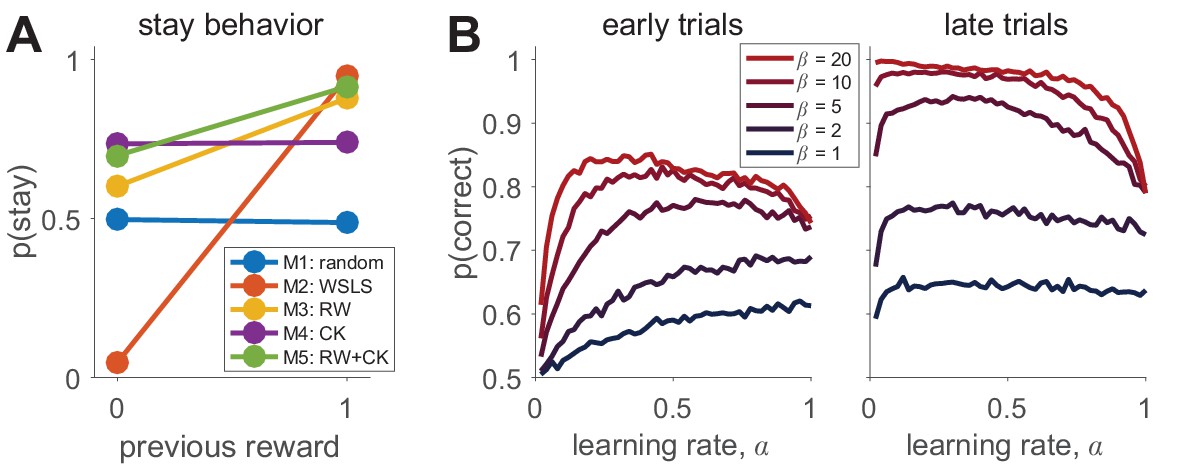
Simulating behavior in the two-armed bandit task.
(A) Win-stay-lose-shift behavior varies widely between models. (B) Model 3 simulations (100 per parameter setting) show how the learning rate and softmax parameters influence two aspects of behavior: early performance (first 10 trials), and late performance (last 10 trials). The left graph shows that learning rate is positively correlated with early performance improvement only for low values or for very low values. For high values, there is a U-shape relationship between learning rate and early speed of learning. The right graph shows that with high values, high learning rates negatively influence asymptotic behavior. Thus, both parameters interact to influence both the speed of learning and asymptotic performance.
Box 3—figure 1
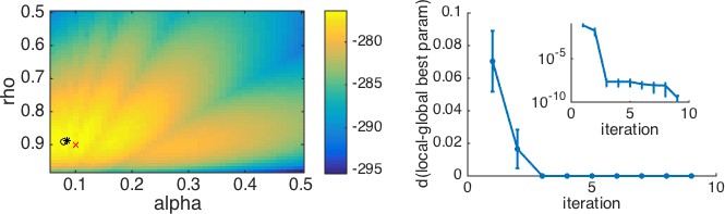
An example with multiple local minima.
(Left) Log-likelihood surface for a working memory reinforcement learning model with two parameters. In this case, there are several local minima, all of which can be found by the optimization procedure depending on the starting point. Red x, generative parameters; black circle, optimum with brute search method; black *, optimum with fmincon and multiple starting points. (Right) Plotting the distance from the best fitting parameters after iterations to the best fitting parameters after all iterations as a function of the number of starting points gives a good sense of when the procedure has found the global optimum. The inset shows the same plot on a logarithmic scale for distance, illustrating that there are still very small improvements to be made after the third iteration.
Box 4—figure 1

Parameter recovery for the Rescorla Wagner model (model 3) in the bandit task with 1000 trials.
Grey dots in both panels correspond to points where parameter recovery for is bad.
Box 5—figure 1

Confusion matrices in the bandit task showing the effect of prior parameter distributions on model recovery.
Numbers denote the probability that data generated with model X are best fit by model Y, thus the confusion matrix represents . (A) When there are relatively large amounts of noise in the models (possibility of small values for and ), models 3–5 are hard to distinguish from one another. (B) When there is less noise in the models (i.e. minimum value of and is 1), the models are much easier to identify. (C) The inversion matrix provides easier interpretation of fitting results when the true model is unknown. For example, the confusion matrix indicates that M1 is always perfectly recovered, while M5 is only recovered 30% of the time. By contrast, the inversion matrix shows that if M1 is the best fitting model, our confidence that it generated the data is low (54%), but if M5 is the best fitting model, our confidence that it did generate the data is high (97%). (D) Similar results with less noise in simulations.
Box 6—figure 1
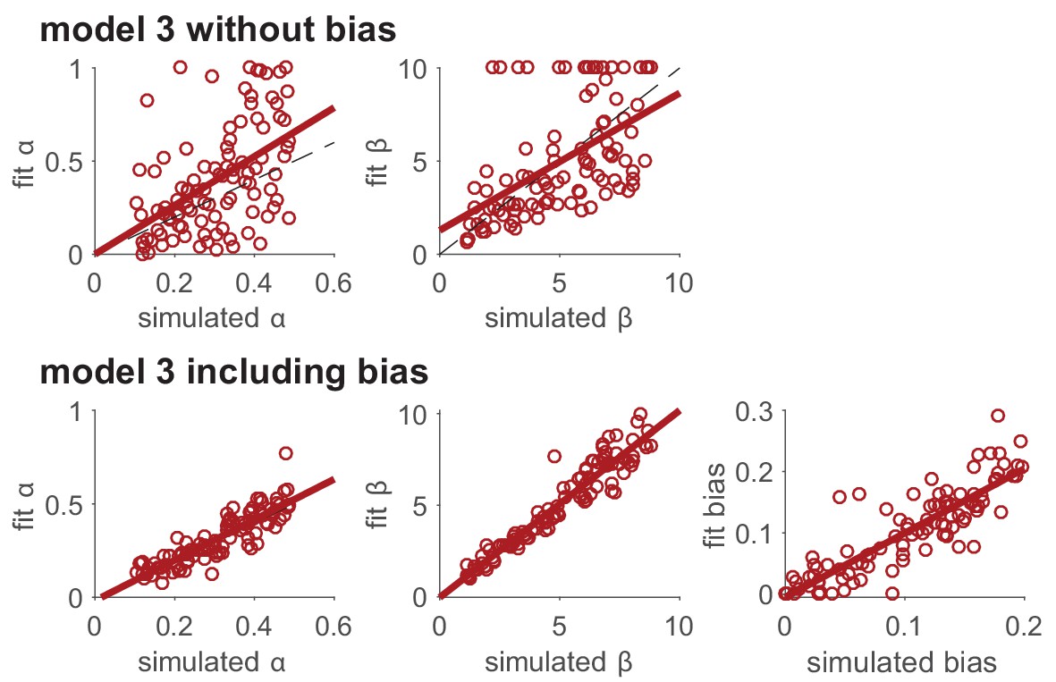
Modeling unimportant parameters provides better estimation of important parameters.
The top row shows parameter recovery of the model without the bias term. The bottom row shows much more accurate parameter recovery, for all parameters, when the bias parameter is included in the model fits.
Box 7—figure 1
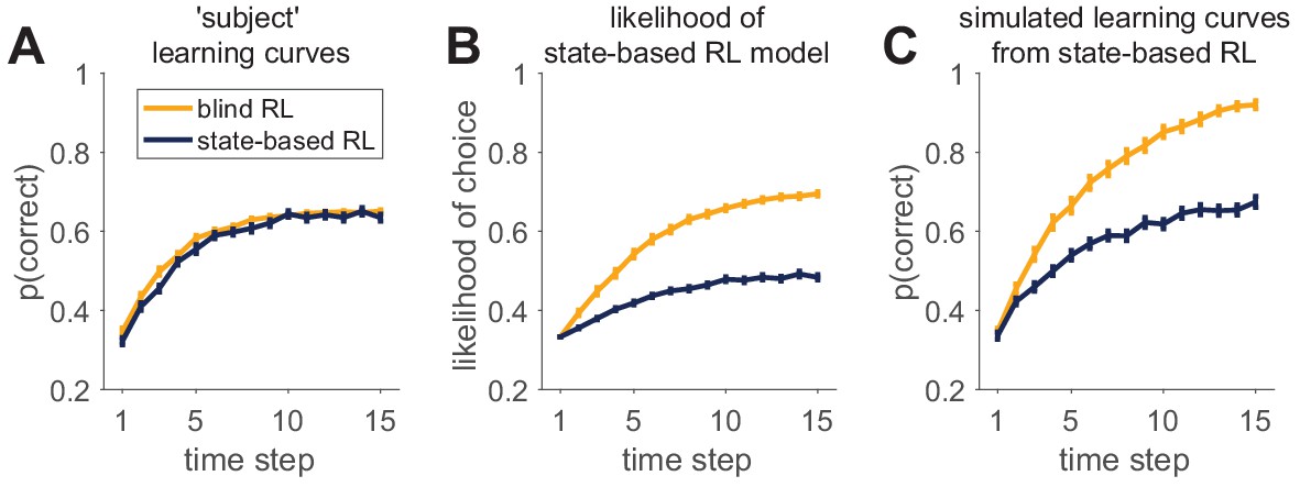
An example of successful and unsuccessful model validation.
(A) Behavior is simulated by one of two reinforcement learning models (a blind agent and a state-based agent) performing the same learning task. Generative parameters of the two models were set so that the learning curves of the models were approximately equal. (B) Likelihood per trial seems to indicate a worse fit for the state-based-simulated data than the blind-simulated data. (C) However, validation by model simulations with fit parameters shows that the state-based model captures the data from the state-based agent (compare dark learning curves in panels A and C), but not from the the blind agent (yellow learning curves in panels A and C).
Download links
A two-part list of links to download the article, or parts of the article, in various formats.
Downloads (link to download the article as PDF)
Open citations (links to open the citations from this article in various online reference manager services)
Cite this article (links to download the citations from this article in formats compatible with various reference manager tools)
Ten simple rules for the computational modeling of behavioral data
eLife 8:e49547.
https://doi.org/10.7554/eLife.49547


