The contribution of temporal coding to odor coding and odor perception in humans
- Bar-Ilan University, Israel
Figures
Figure 1 with 1 supplement
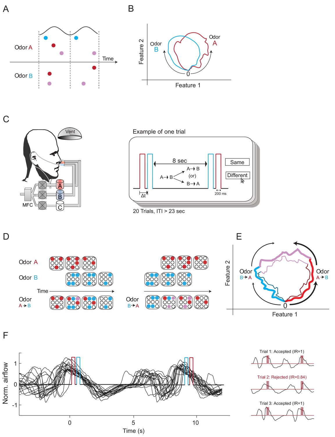
Construction of odors differing mainly in their odor-elicited temporal dynamics.
(A) A schematic diagram showing three glomeruli (colored circles) responding to two odors over two cycles of a putative oscillatory mechanism (black line). Odors A and B activate the same glomeruli but at different times. According to the Hopfield model, this difference in activation time should be sufficient to render these two odor codes as different odors. (B) Two odor trajectories plotted in phase space. The two trajectories represent two different odors as their trajectories are different in phase space. (C) Left panel: experimental setup. Participants were presented with two odors dispensed from two separate canisters using a computer-controlled air dilution olfactometer. Another canister was used to deliver clean air (marked as C). Nasal respiration was recorded using a nasal cannula attached to a pressure-sensitive spirometry sensor. Right panel: experimental design. Two odor pulses were presented consecutively spaced by a time delay (Δt) between them. Eight seconds later, we presented either the same order of odor presentations or a reversed one. Participants then reported whether the odors were the same or different. Twenty-three seconds later, this procedure was repeated. Each participant underwent 20 trials. Red, odor A; blue, odor B; ITI, inter-trial-interval. (D) A mockup model of glomeruli responses to two odors delivered one after the other with a short delay in between, both in forward and in reverse order. Red and blue circles represent glomeruli activated by odors A and B, respectively. Purple circles represent glomeruli activated by odors A+B. The order of odor presentation elicits different time sequences of glomeruli activation. (E) Possible trajectories of the two TOMs in phase space. The first trajectory (thick lines) is composed of odor A (red), odors A+B (purple) and then odor B (blue). The second trajectory (thin lines) represents odor B, odor B+A, and odor B. The two trajectories are relatively similar, although the directions are opposite. (F) A typical example of a 20-trial experimental session. Left panel: black traces depict several typical nasal respiration trials overlaid. Positive values represent inhalation. Red and blue triggers represent a single example of odor A and B pulses. Right panel: examples of trials in which the TOMs were presented entirely concurrent (top and bottom) or not concurrent (middle) with sniffing.
Figure 1—figure supplement 1
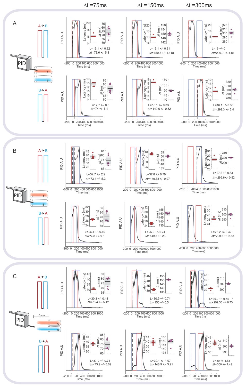
Setup validation.
(A) Photo-ionizer detector (PID) measurements of the TOMs and their components at several delays. PID location was close to the tube carrying odor A (red) and therefore reports only odor A. Recordings were made using the exact same parameters as in the psychophysical experiment. Red and blue rectangular triggers denote the valve-opening signals of odor A and B, respectively. The top row shows PID response to an AB TOM, whereas the bottom row shows the same for a BA TOM. Black trace and gray shading are the mean PID responses and their standard error (SEM; N = 10). PID responses are normalized to a maximal value of 1 and are denoted in arbitrary units (A.U). Time 0 is the time of first valve opening per TOM. The mean latency between trigger onset and the time at which PID response reaches 10% of the maximal value is marked by a dashed black line. Left, center and right panels depict a time delay (Δt) of 75, 150, and 300 ms between TOM constituents, respectively. Within each panel, two scatter plots are overlaid: latency (red, the time it takes the signal to reach 10% of its maximum) and Δt (purple, the time of the second odor pulse). In each plot, the mean and SEM 95% confidence interval are displayed in black and gray, respectively. Individual data points per trial (N = 10) are also shown. Mean ± SEM values also appear as text below the plots. (B) The same as panel (A), but for PID location within the pipe carrying odor B (cinnamon). (C) The same as panels (A) and (B) but for a PID location 5 cm away from the joint location of the odor ports, to mimic the average location of the participants’ nose. At this location, the PID registers signals of both odors. Note that in order to account for the difference in PID response between odorants, here plotted together, the mean latency between trigger onset and the time of PID response was measured for the time taken to reach the 5% of maximal value.
Figure 2 with 1 supplement

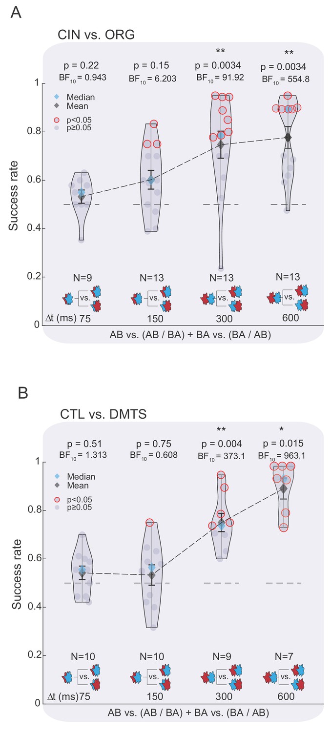
Participants could not discriminate between TOMs composed of two familiar odors.
(A) Violin graph of the success rates of individual participants in discriminating between TOMs composed of ORG and CIN with Δt = 300 ms and Δt = 600 ms. Gray data points represent the success rate of an individual participant. Participants who scored significantly higher than chance are circled in red (p<0.05 binomial test, uncorrected for multiple comparisons). Means and medians are marked by black and blue diamonds, respectively. Standard deviation around the mean is marked in black. The result of a two-sided sign test, comparing the median success rate to the expected chance success rate of 0.5, and the Bayesian statistics are denoted above each group. Overlapping data points are shifted sideways across the x axis for visualization purposes. The dashed line marks the chance success rate (0.5). The number of participants in each group is denoted by N. Left violet box: participants’ success rates for the TOM experiments. Right gray box: results of four control experiments validating that failure to discriminate between TOMs is not due to suboptimal choice of experimental parameters or odor delivery system. Note that in all control experiments, the majority of the cohort performed significantly above chance and the mean and median success rates were significantly above chance level. *, ** and *** represent p<0.05, p<0.01 and p<0.001, respectively (same applies for all figures in this manuscript). (B) Success rates of the TOM discrimination experiment split into trials in which the TOMs presented were the same or when they were different (Δt = 300 ms). No significant difference was detected between the two group means (two-tailed t-test, t(9) = −0.11 p=0.91). (C) Equally perceived intensity of the odors constituting the TOMs. The bar graph depicts the mean perceived intensity of the odors used (ORG and CIN). Error bars are the standard errors of the means. Gray dots denote the individual participant success rates. No significant difference was detected between the two group means (two-tailed t-test, t(10) = −0.45 p=0.66).
-
Figure 2—source data 1
Discrimination between TOMs comprised of CIN and ORG.
- https://cdn.elifesciences.org/articles/49734/elife-49734-fig2-data1-v1.xlsx
Figure 2—figure supplement 1
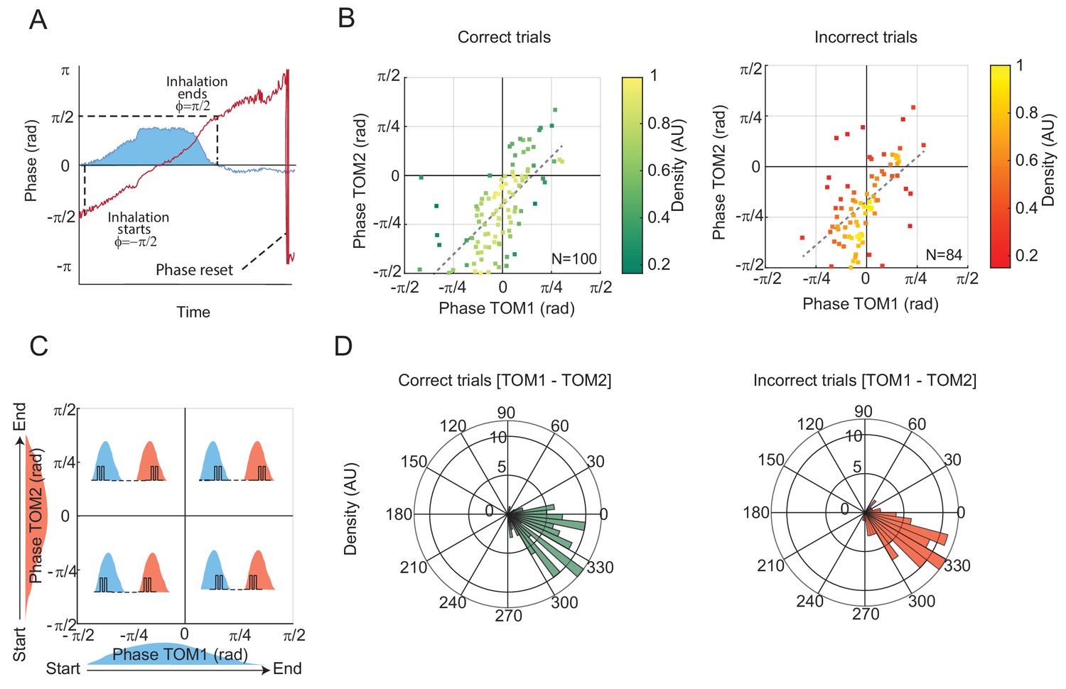
Phase analysis.
(A) Respiratory phase was calculated with MATLAB’s ‘angle’ function applied to the Hilbert transform of the respiratory trace. The product of this calculation is the phase, which gradually increases from –π/2 to π/2 over the course of the inhalatory phase of the respiratory cycle. (B) Distribution of the respiration phases in which the first and second TOMs occurred. The data are divided into correct (green, left panel) and incorrect (red, right panel) trials. The color bar indicates the density of the respiratory phase values. (C) A schematic example of four possible phase differences for the first TOM (blue) and the second TOM (red). (D) Polar histogram of the differences between the first and second TOMs. Binned data are divided into correct (green, left panel) and incorrect (red, right panel) trials.
Figure 3 with 1 supplement
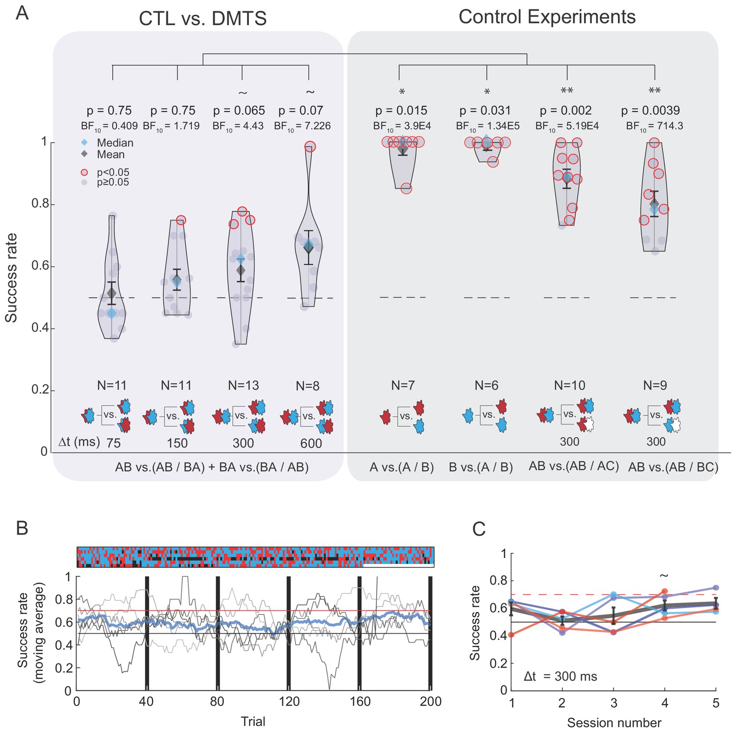
The majority of the participants could not discriminate between TOMs that are composed of highly dissimilar odors.
(A) Left box: success rates for discrimination between TOMs composed of CTL and DMTS as a function of Δt. Color code as in Figure 2. Gray right box: four control experiments demonstrating that the vast majority of participants can discriminate between the constituent odors or TOMs when one of the odors is clean air (labeled as C). '~' denotes marginally significant (p>0.05 and p<0.07). (B) Extensive training does not substantially improve discrimination between TOMs. Lower panel: discrimination score progression over five sessions of 40 trials each. Participants who reached and maintained a score benchmark of 0.7 (red horizontal line) in one session ended their participation and they did not return for additional sessions. Chance performance (0.5) is marked by a black horizontal line. Thin gray lines mark individual participants and the thick blue line is the average of all participants over a moving window of 20 trials. The upper panel reflects trial-by-trial performance (columns) per participant (rows), where the color of each tile denotes accuracy: correct (blue), incorrect (red), or removed because the odor presentation was not in sync with sniffing (black). (C) Mean success rate for each participant across the five sessions. Group mean per session is depicted by a thick gray line along with vertical bars representing the standard error.
-
Figure 3—source data 1
Discrimination between TOMs comprised of CTL amd DMTS.
- https://cdn.elifesciences.org/articles/49734/elife-49734-fig3-data1-v1.xlsx
Figure 3—figure supplement 1

Analysis of the percept elicited by different odor constituents used in TOMs.
(A) Projection of verbal descriptor ratings onto the two main axes of principal component space for ORG (orange), CIN (brown), CTL (red), and DMTS (blue). Each data point represents the ratings of a single participant for a given odor (N = 8). The centroids of each cluster are marked by labeled circles following the same color scheme. (B) Perceived distance of TOM constituents across participants and odors. A matrix comprised of the Euclidean distance between eleven descriptor ratings provided by individual participants for each odor. Hotter colors denote larger distances. Ratings are divided into four odorant subgroups by a black grid. Mosaic-like patterns within each compartment represent between-participant variability in ratings of the same odor. (C) CTL and DMTS are perceived more differently than ORG and CIN. Bars depict mean of the Euclidean distance between two pairs of odors – CTL and DMTS (left) and CIN and ORG (right). Error bars are the standard errors of the means. (D) Equally perceived intensity of the odors constituting the TOMs. Bars depict the mean perceived intensities of the odors used (CTL and DMTS). Error bars denote the standard errors of the means. Each gray point denotes the rating of one participant.
Figure 4 with 1 supplement

Perception of TOMs is an intermediate of that of their components.
(A) Projection of verbal descriptor ratings of the four odors onto the two main axes of principal component space for CTL (labeled 'A', red circles), DMTS (labeled 'B', blue circles) and two TOMs comprised of CTL and DMTS presented in two temporal sequences: (brown) and (purple). Each data point represents the ratings of a single participant for a given odor or TOM. The centroids of each cluster are marked by labeled circles following the same color scheme. (B) A matrix comprised of the Euclidean distances between eleven descriptor ratings provided by the participants for CTL (labeled ‘A’), DMTS (labeled ‘B’) and two TOMs comprised of CTL and DMTS. Hotter colors denote larger distances. Ratings are divided into four odorant subgroups by a black grid. Mosaic-like patterns within each compartment represent the between-participant variability of ratings for the same odor. (C) TOMs are perceived more similarly to each other than to their isolated constituents. Bar graph of mean perceptual distance between TOMs ( or ) and their constituent odorants (A and B). Statistical significance is denoted for post-hoc comparisons of perceptual distance between the monomolecular constituents ('A vs. B') with all other stimuli in black and for the TOMs with all other stimuli in red. Error bars are mean ± SEM. (D–F) Same as panels (A–C) for Δt = 600 ms.
-
Figure 4—source data 1
Olfactory verbal descriptors for TOM perception.
- https://cdn.elifesciences.org/articles/49734/elife-49734-fig4-data1-v1.xlsx
Figure 4—figure supplement 1
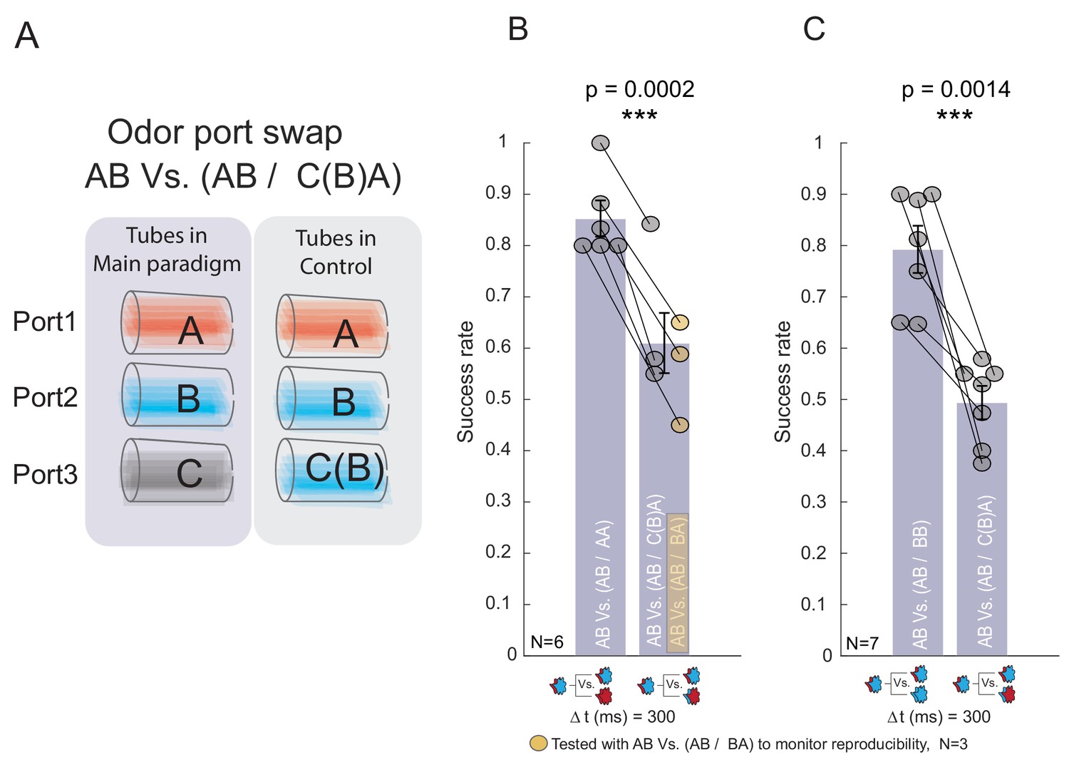
Additional control experiments.
(A) Schematic illustration of the odor port swap paradigm. (B) The success rate of six participants in two experiments. Each participant conducted both experiments in random order. The first experiment was AB vs. (AB/AA) and the second experiment was AB vs. (AB/C(B)A), where C(B) stands for odor B delivered through port C (previously used to deliver air). Participants succeeded in the first experiment but failed in the second. This demonstrates that they could discriminate between TOMs if they differed in odor content, despite having the same duration, but could not discriminate between two TOMs, even if one of the TOMs was delivered through different pipes. Black lines connect data points for each participant between paradigms. (C) Same as panel (A) when using odor BB instead of AA.
Figure 5
Temporal odor dynamics can be used to extract odor-related information.
(A) Success rate of discrimination between the TOMs constituting the ORG and CIN odors as a function of Δt when participants were aware of the constituent odors and their temporal features. Color and legend code as in Figure 2. (B) Same as in panel (A), but for the TOMs composed of CTL and DMTS.
-
Figure 5—source data 1
Discrimination between TOMs when aware of temporal features.
- https://cdn.elifesciences.org/articles/49734/elife-49734-fig5-data1-v1.xlsx
Additional files
Download links
A two-part list of links to download the article, or parts of the article, in various formats.
Downloads (link to download the article as PDF)
Open citations (links to open the citations from this article in various online reference manager services)
Cite this article (links to download the citations from this article in formats compatible with various reference manager tools)
The contribution of temporal coding to odor coding and odor perception in humans
eLife 9:e49734.
https://doi.org/10.7554/eLife.49734


