Figures and data in Noninvasive quantification of axon radii using diffusion MRI

Figures
Tables

15 figures and 1 table

Figures

Figure 1

Download asset Open asset

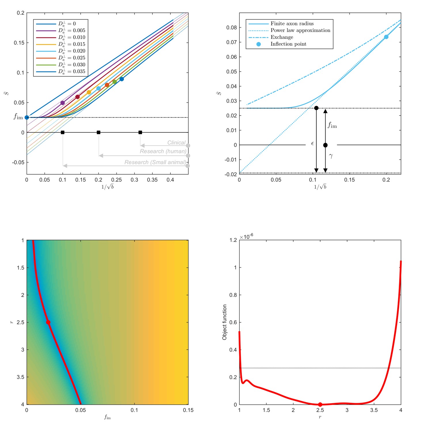
Breakdown of power law scaling: Top left: A nonzero $D_{a}^{⟂}$ would result in a truncated power-law signal decay.

Although the resulting signal nonlinearity might be too subtle to be discerned within the achievable $b$ -range, even for (pre-)clinical systems with strong diffusion-weighting gradients, the *concavity* of the curves plotted as function of $ξ = 1 / \sqrt{b}$ for $ξ > ξ_{*} = \sqrt{2 D_{a}^{⟂}}$ means that even the smallest $D_{a}^{⟂}$ will result in an extrapolated $ξ \to 0$ intercept $γ < f_{im}$ when the power law, Equation 1, is used to approximately describe the signal in the delineated $b$ -ranges. The intercept is maximally negative at the inflection point $ξ_{*}$ (colored dots), beyond which each curve becomes convex, and the negative intercept $γ$ of the linear extrapolation starts to decrease. In all plots here, diffusivities and $b$ -values are expressed in µm²/ms and ms/µm², respectively. Top right: One representative curve ( $D_{a}^{⟂} = 0.020$ ) is shown to highlight the differences between the physically plausible dot compartment $f_{im} > 0$ , and the intercept $γ$ . The dot compartment is a positive signal fraction of a biophysical compartment, whereas the intercept is a parameter of the power-law approximation, Equation 1. Their difference $ϵ$ depends on various parameters, including the axonal signal fraction, diffusivities, the axon radius, and the scan protocol. The predicted signal decay for the exchange model (dash-dotted; Equation 4) is convex in the entire $b$ -range, where the signal decay for the finite axon radius model (dotted; Equation 2) is concave until the inflection point. Bottom: The optimization landscape of Equation 3 shows a shallow valley, relative to the noise floor, for a simulation that mimics the human component of the study. (Bottom left) The valley is shown in a 2D projection of the landscape (shown as a function of radius instead of $D_{a}^{⟂}$ , see Equation 10). (Bottom right) The fit objective function along the valley is shown (red line) in comparison to the noise floor (dashed line) with an unrealistically high SNR of 250 for the non-DW signal. The red dot indicates the ground truth value.

Figure 2

Download asset Open asset

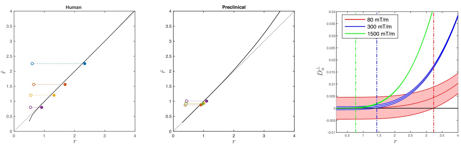
Simulations on accuracy and precision of MR-based axon radius mapping.

First, the left and middle panel show the difference between the estimated, $\hat{r}$ , and theoretical, $r$ , effective MR radius associated with various realistic axon caliber distributions (*solid dots* with different color for different distributions) for the clinical and preclinical setups, respectively. Axon caliber distributions were adopted from Aboitiz et al. (1992) and Innocenti et al. (2015) for the clinical simulations (see Figure 7), whereas various axon distributions (see Figure 4) derived from our own histology were used for the preclinical simulation. The average radii, $\bar{r}$ , of the axon caliber distribution are shown for comparison (*open dots*). Additionally, the accuracy of the framework for a system with single cylinder with radius $r$ is shown (*black line*). Second (right figure), the feasibility to measure $D_{a}^{⟂}$ with statistical significance in case of scan settings and SNR for the Connectom (300 mT/m; blue), Aeon (1500 mT/m; green) protocol, respectively. For comparison, we also assessed the feasibility for the Prisma protocol as described in Veraart et al. (2019) (80mT/m; red). The shaded areas illustrate the 95% confidence intervals derived from Cramér-Rao lower bound analysis of model, Equation 2 with $f_{im} = 0$ . The corresponding minimal cylinder radius $r$ that allows for the observation of significant $D_{a}^{⟂} (r)$ , $r = 0.76 μ m$ , 1.41 µm and 3.24 µm for Aeon, Connectom, and Prisma, respectively, is indicated by the vertical lines. In all plots, diffusivities and radii are expressed in $μ m^{2} / m s$ and $μ m$ , respectively.

Figure 3

Download asset Open asset

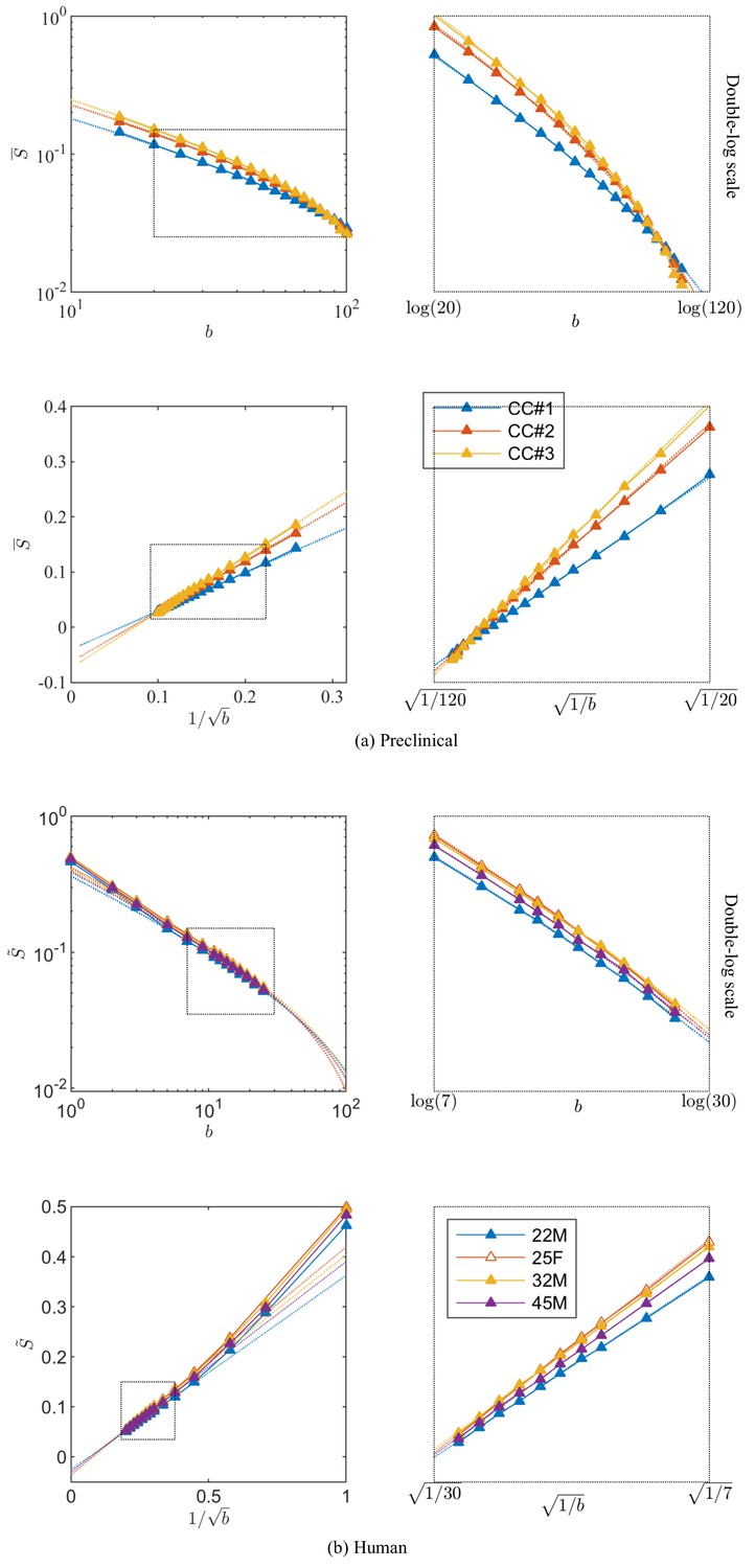
Breaking of the power law.

The ROI- and spherically averaged signal decay is shows for the different fixed samples of the rat CC (a) and human subjects (b) and as a function of $1 / \sqrt{b}$ and on a double logarithmic scale. The data deviate from the power law scaling with exponent 1/2 that is predicted by the stick model (i.e. nonlinear signal decay in log-log plot), thereby demonstrating sensitivity of the signal to the radial intra-axonal signal. The fits of Equation 1 are shown in dashed lines. In all plots, $b$ is expressed in $m s / μ m^{2}$ .

Figure 4

Download asset Open asset

Histological validation, part I.

The axon radius distributions for different ROIs of rat CC#1 are shown (blue bars).The associated tail-weighted effective radii are shown in the black lines, whereas the corresponding MR estimates are shown by the red lines. In all plots, $r$ is expressed in $μ m$ .

Figure 5

Download asset Open asset

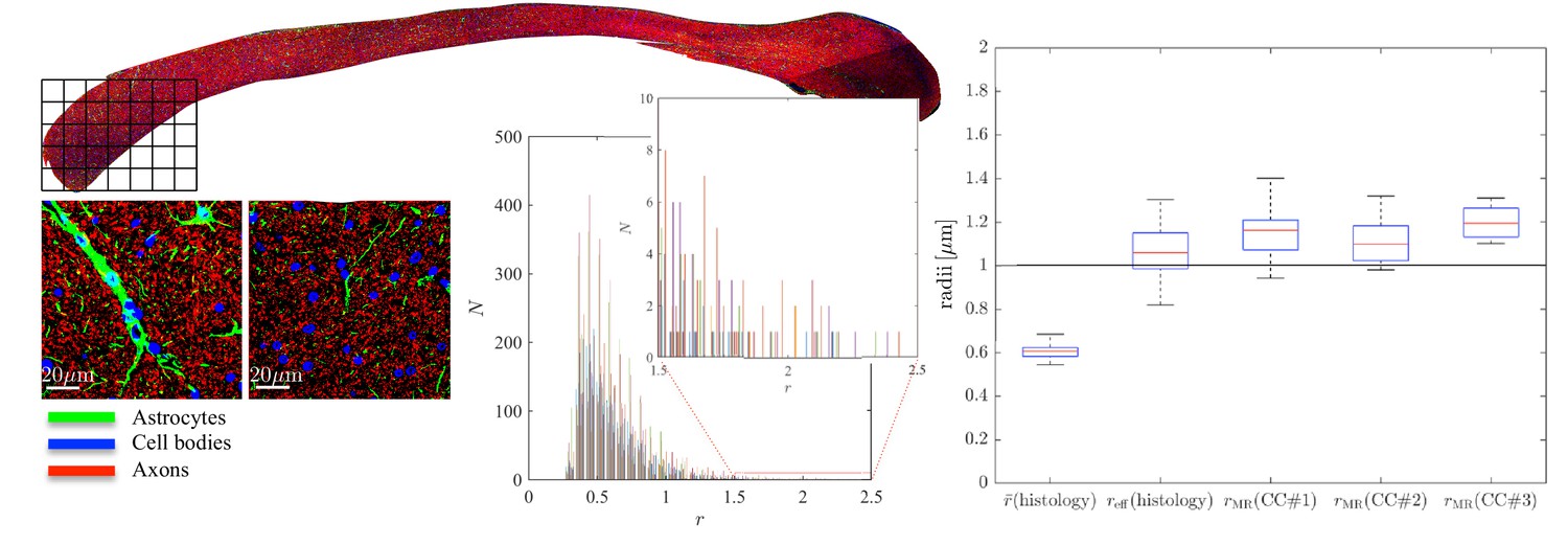
Histological validation, part II.

(left) For a second fixed brain sample, CC#2, the confocal microscopy images, stained for neurofilaments (red), astrocytes (green), and cell bodies (blue), are shown for two representative $100 \times 100 μ m^{2}$ -patches that are positioned within the Genu (microscopy image of CC shown for ROI positioning). The abundance of astrocytes and cell bodies, both representing 5% of the volume, is clear in both patches. The astrocytic processes can have a large diameter, up to 7 µm in the first patch. A detailed analysis of the radius distribution of the astrocytic processes is not possible due to their random orientation w.r.t. the image plane. (middle) Axon radius distributions for all 16 patches of the Genu (each patch has different color in the bar plot). (right) Boxplots represent the distribution of the average and effective radius of the axon radii distribution that were extracted from each of the 16 patches within the genu. The effective radius $r_{eff}$ is larger than the average $\bar{r}$ , respective medians are 1.06 and 0.61 µm. The boxplots for the MR-derived axon radius measurements for 16 MR voxels within the genu for the three fixed CC samples are also shown. In all plots, radii are expressed in $μ m$ .

Figure 6

Download asset Open asset

Effective radii in the CC.

Maps of the effective radii derived from diffusion MR data, for the 3 samples of the rat CC.

Figure 7

Download asset Open asset

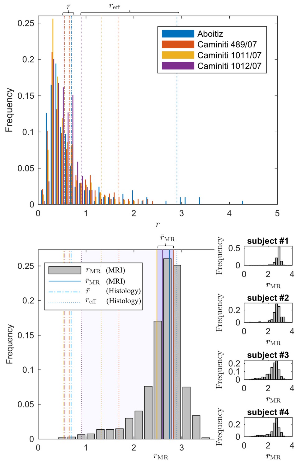
Comparing the effective radius from histology and in vivo dMRI.

(top - histology) Axon radius distributions of multiple histological studies and human CC samples show a good correspondence for the bulk of the distribution, represented by the average radius $\bar{r}$ (dashed-dotted lines). Due to mesoscopic fluctuations of the large axons in histological samples, the corresponding effective radius $r_{eff}$ dominated by large axons, shows strong variability (dotted lines). (bottom - MRI) The four Connectom subjects show good correspondence in terms of $r_{eff}$ . The distribution describing $r_{eff}$ for all voxels in the midbody of the CC for all four subjects falls almost entirely within the range spanned by values predicted by histology, with no need to account for potential shrinkage (Horowitz et al., 2015) during tissue preparation. In all plots, radii are expressed in $μ m$ .

Figure 8

Download asset Open asset

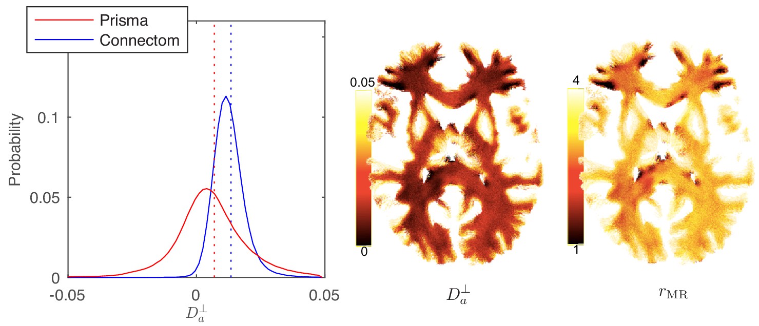
Distribution and maps of $D_{a}^{⟂}$ and $r_{MR}$ .

(left) The distribution of $D_{a}^{⟂}$ estimated via Equation 3 for all WM voxels (all scanner-specific subjects pooled) shown for both scan set-ups. In agreement with Figure 2, Prisma (80mT/m) data shows a much lower precision for the estimator of $D_{a}^{⟂}$ . Despite the small yet positive mean value and the associated negative offset $γ$ in Figure 3, a large number of WM voxels yield biophysically implausible $D_{a}^{⟂} < 0$ values. Precision drastically improves on the Connectom scanner (300 mT/m). (right) Maps of $D_{a}^{⟂}$ , and of the effective MR radius heavily weighted by the tail of axonal distribution (Figure 7), for a single subject. Here, $r_{M R}$ is derived from $D_{a}^{⟂}$ via Equation 10. In all plots, diffusivities and radii are expressed in $μ m^{2} / m s$ and $μ m$ , respectively.

Figure 9

Download asset Open asset

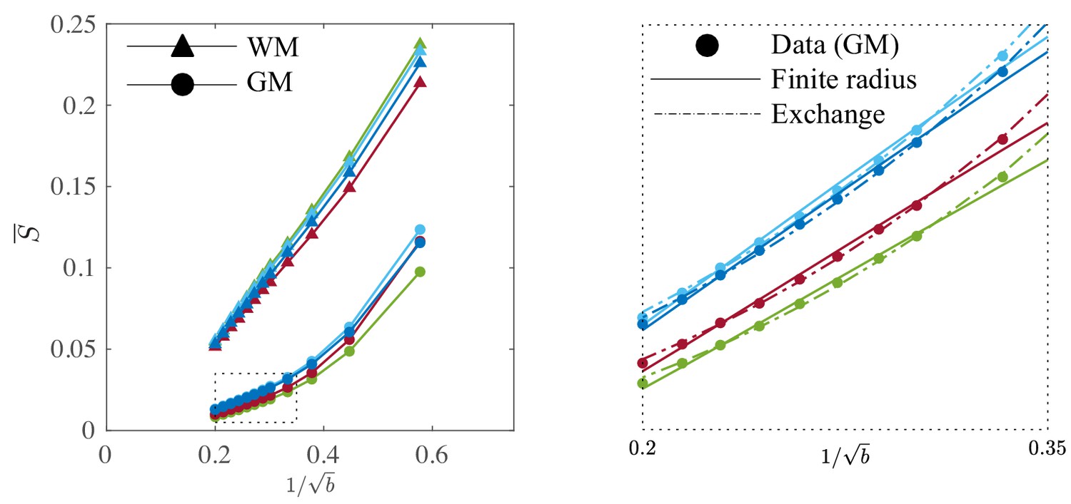
Signal decay in the GM.

The spherically-averaged signal decay in the WM and GM is shown for all human subjects as a function of $1 / \sqrt{b}$ . The consistent non-linear scaling of the signal as a function of $1 / \sqrt{b}$ demonstrates deviations from the ‘stick’ model in the cortical GM. In contrast to the WM, the convex signal decay in the GM is better described by an anisotropic exchange model of two compartments (Equation 4), than the finite radius model (Equation 3). In all plots, $b$ is expressed in $m s / μ m^{2}$ .

Figure 10

Download asset Open asset

Raw data.

The spherically-averaged diffusion-weighted images, prior to any other image corrections, are shown for various low and high $b$ -values for one rat brain sample (a) and one human subject (b).

Figure 11

Download asset Open asset

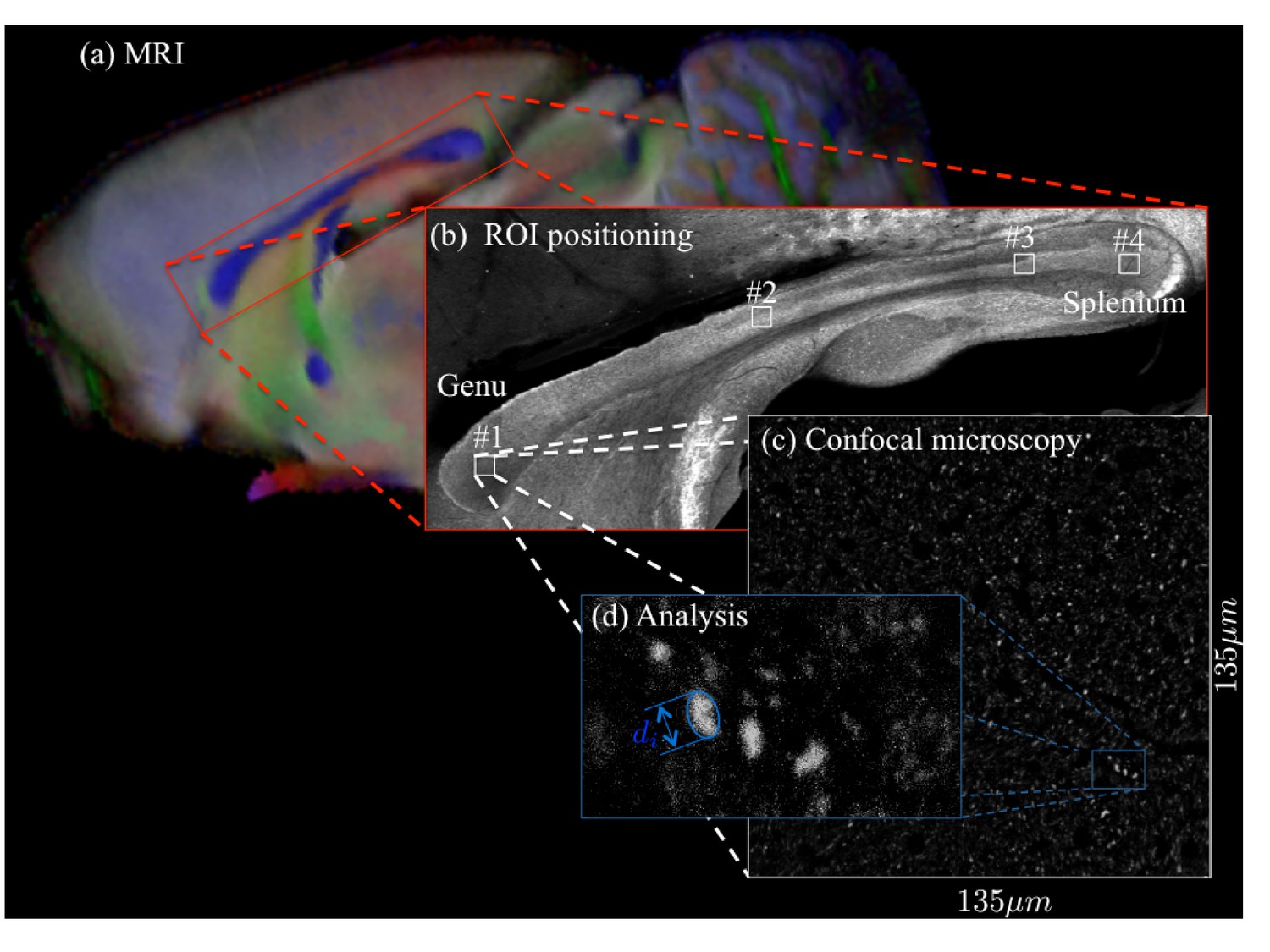
For two brain samples, MR scanning (a, color encoded FA map) was followed by low (b) and high (c) resolution confocal microscopy with staining for neurofilaments to identify the axons.

The low-resolution image was used to position various ROIs, whereas the axon caliber distributions were extracted from the high-resolution image of the corresponding ROIs. The long axes of fitted ellipsoids served as proxies for the respective axon diameters (d).

Author response image 1

Download asset Open asset

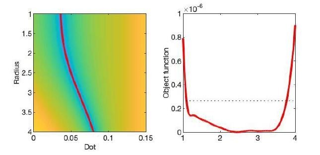
The optimization landscape of model (III) shows a shallow valley, relative to the noise floor, for a simulation that mimics the human component of the study.

(left) The valley is shown in a 2D projection of the landscape (plot shown as a function of radius instead of D_a^perp). (right) The fit objective function along the valley is shown (red line) in comparison to the noise floor with an unrealistically high SNR of 250 for the non-DW signal.

Author response image 2

Download asset Open asset

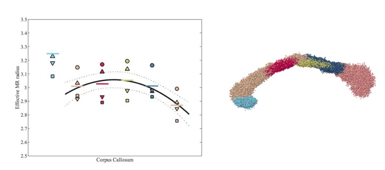
Effective MR radius for various segments of the human CC, including rostrum (light blue) and genu to splenium (from left to right), for each of the 4 subjects.

Each subject is represented by a subject-specific marker. The segmentation of the CC is shown on the right hand side.

Author response image 3

Download asset Open asset

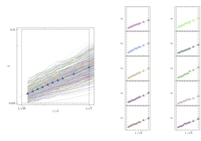
Signal decay in a single voxel.

(left) The spherically-averaged signal decay is shown as a function of $1 / \sqrt{b}$ for all individual voxels of the WM of one human subject (faded colored lines) and for the average across all WM voxels (blue line with markers, Figure 5B). (right) The signal decay for individual voxels is shown for 10 arbitrarily-chosen WM voxel. The dashed box is positioned the same for all graphs.

Author response image 4

Download asset Open asset

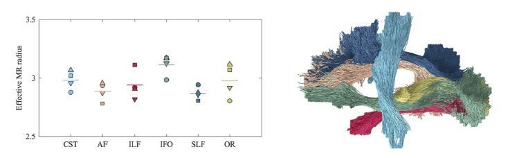
Average effective MR radius within various tracts (color encoded as shown on the right; both hemispheres were considered simultaneously) for the 4 human subjects (encoded by marker).

The line segments show the mean across the subjects. The inter-tract variability exceeds the inter-subject variability. We hypothesize that the hereby introduced technique can be used in future studies to characterize the typical, developing, or pathological brain in a wide range of species, including humans, rodents, or non-human primates.

Tables

Key resources table

Reagent type (species) or resource	Designation	Source or reference	Identifiers	Additional information
Antibody	anti-Neurofilament 160/200 (Mouse monoclonal)	Sigma Aldrich	Cat# N2912 (clone RMdo20)	2.5 µg/mL
Antibody	anti-GFAP (rabbit polyclonal)	Thermo Fisher Scientific	Cat# PA1-10019	1:1000
software. algorithm	ImageJ	imagej.nih.gov/ij/	RRID: SCR003070	1.52q
software. algorithm	FSL	fsl.fmrib.ox.ac.uk/fsl/	RRID: SCR002823	v6
software. algorithm	MRtrix	www.mrtrix.org	RRID: SCR006971	v3.0
software. algorithm	FreeSurfer	surfer.nmr.mgh.harvard.edu	RRID: SCR001847	v6.0.0
Other	DAPI	Sigma Aldrich	Cat# D9542	500nM

Download links

A two-part list of links to download the article, or parts of the article, in various formats.

Downloads (link to download the article as PDF)

Article PDF

Open citations (links to open the citations from this article in various online reference manager services)

Mendeley

Cite this article (links to download the citations from this article in formats compatible with various reference manager tools)

Jelle Veraart
Daniel Nunes
Umesh Rudrapatna
Els Fieremans
Derek K Jones
Dmitry S Novikov
Noam Shemesh

(2020)

Noninvasive quantification of axon radii using diffusion MRI

eLife 9:e49855.

https://doi.org/10.7554/eLife.49855

Share this article

Cite this article

Breakdown of power law scaling: Top left: A nonzero Da⟂ would result in a truncated power-law signal decay.

Simulations on accuracy and precision of MR-based axon radius mapping.

Breaking of the power law.

Histological validation, part I.

Histological validation, part II.

Effective radii in the CC.

Comparing the effective radius from histology and in vivo dMRI.

Distribution and maps of Da⟂ and rMR.

Signal decay in the GM.

Raw data.

For two brain samples, MR scanning (a, color encoded FA map) was followed by low (b) and high (c) resolution confocal microscopy with staining for neurofilaments to identify the axons.

The optimization landscape of model (III) shows a shallow valley, relative to the noise floor, for a simulation that mimics the human component of the study.

Effective MR radius for various segments of the human CC, including rostrum (light blue) and genu to splenium (from left to right), for each of the 4 subjects.

Signal decay in a single voxel.

Average effective MR radius within various tracts (color encoded as shown on the right; both hemispheres were considered simultaneously) for the 4 human subjects (encoded by marker).

Downloads (link to download the article as PDF)

Open citations (links to open the citations from this article in various online reference manager services)

Cite this article (links to download the citations from this article in formats compatible with various reference manager tools)

Breakdown of power law scaling: Top left: A nonzero $D_{a}^{⟂}$ would result in a truncated power-law signal decay.

Distribution and maps of $D_{a}^{⟂}$ and $r_{MR}$ .