Cortical excitability controls the strength of mental imagery
- School of Psychology, University of New South Wales, Australia
- Department of Neurophysiology, Max Planck Institute for Brain Research, Germany
- Brain Imaging Center Frankfurt, Goethe-University Frankfurt, Germany
Figures
Figure 1 with 2 supplements
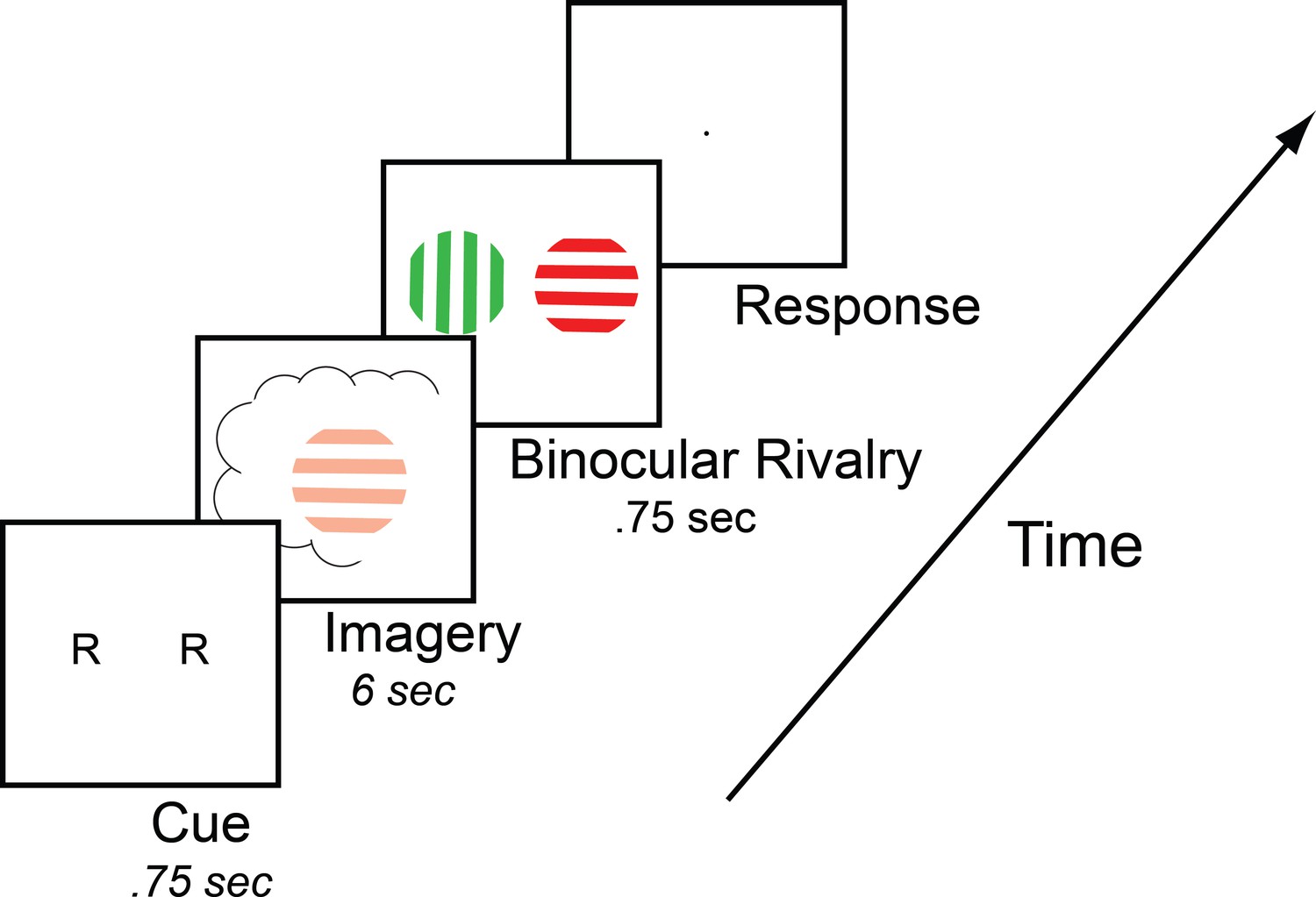
Timeline of the basic imagery experiment.
Participants were cued to imagine a red-horizontal or a green-vertical Gabor patch for 6–7 s by the letter R or G (respectively). Following this, they were presented with a brief binocular rivalry display (750 ms) and asked to indicate which image was dominant. In the behavioral experiments with the brain-imaging sample and in three of the tDCS experiments, a rating of subjective vividness of the imagery also preceded the binocular rivalry display.
Figure 1—figure supplement 1
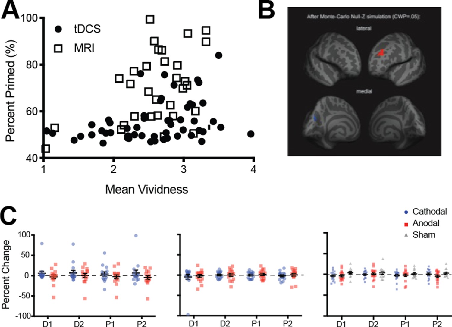
Imagery vividness results.
(A) Data shows the correlation between mean vividness ratings (x-axis) and visual imagery priming (y-axis) for participants from both the MRI and tDCS experiments (tDCS experiments 2, 3 and 4). All possible participants’ data were included for the tDCS analysis (resulting in the analysis of 54 participant’s data). Only the correlation in the tDCS sample was significant, (rs = 0.37, p=0.003, Spearman’s rank-order correlation was used due to a violation of normality). The effect size was too small for significant results in the fMRI sample (rs = 0.34, p=0.065, Spearman’s rank-order correlation was used due to a violation of normality, N = 31). (B) Surface-based whole brain analysis of the fMRI resting-state data: associations with subjective vividness. Corrected clusters showing associations with individual subjective vividness at a cluster-wise probability threshold of p<0.05 (see also see Supplemental Table S3). The upper row shows a lateral view of the two hemispheres from an anterior perspective, whereas the lower row shows a medial view of them from the back. Multiple comparison correction was done using Monte Carlo Null-Z simulation (mc-z). No smoothing of the functional data was applied. Only two fMRI mean intensity clusters showed associations with subjective vividness that survived the correction for multiple comparisons: One cluster in the left rostralmiddlefrontal cortex showed a positive association (orange), and one smaller cluster in the left cuneus showed a negative association (blue). Note the similarity in the subjective vividness results with the ones in Bergmann et al. (2016b), where only a volume cluster in left frontal cortex also showed a positive association with subjective vividness. Apparently, the positive relationship of subjective vividness with the anatomy of left frontal cortex is also reflected in the fMRI mean intensity levels of this region. (C) tDCS effect on mean vividness ratings. Left panel: Occipital (1.5ma) – Vividness ratings were included in this experiment, which allowed us to look at subjective changes in imagery vividness that occur with changes in cortical excitability of the visual cortex. Red dots show the effect of anodal stimulation (increasing excitability) while blue dots show cathodal stimulation (decreasing excitability). Each dot represents an individual participant (one participant’s data is excluded from this analysis due to incorrect button presses on one of the days of testing, N = 15). All data show means and error bars represent ± SEM’s. The data was again analyzed using percentage changed. We found no significant differences in the reported mean vividness of the imagined patterns (main effect of tDCS polarity: F(1,14) = 1.97, p=0.18, main effect of block: F(3,42) = .73, p=0.54, interaction: F(3,42) = .59, p=0.63). Middle panel: tDCS of prefrontal cortex and mean vividness ratings. As vividness ratings were included in this experiment, we could also look at the subjective changes in imagery vividness that occur with changes in cortical excitability of the prefrontal cortex. Red dots show the effect of anodal stimulation (increasing excitability) while blue dots show cathodal stimulation (decreasing excitability). All data show means and error bars represent ± SEM’s. We again analyzed the data using the percent change scores. There were no differences in the mean vividness ratings for either polarity of the tDCS (main effect: F(1,15) = .28, p=0.61) or the block (main effect: F(3,45) = .77, p=0.51), and there was no interaction between the two (F(3,45) = .07, p=0.98). Right panel: tDCS of occipital cortex (1.5ma) – cathodal, anodal and sham stimulation, one participant's data is removed due to incorrect button presses for vividness ratings. Red dots show the effect of anodal stimulation (increasing excitability) while blue dots show cathodal stimulation (decreasing excitability), and grey triangles show the effect of sham stimulation. All data show means and error bars represent ± SEM’s. We again analyzed the data using the percent change scores. There were no differences in the mean vividness ratings for any of the polarity conditions (Mixed-effects analysis due to attrition: Polarity effect: F(1.95, 31.19)=1.38, p=0.27), there was also no effect of block (F(2.19, 34.98)=0.94, p=0.41) and no interaction (F(2.63, 36.82)=0.98, p=0.41).
Figure 1—figure supplement 2
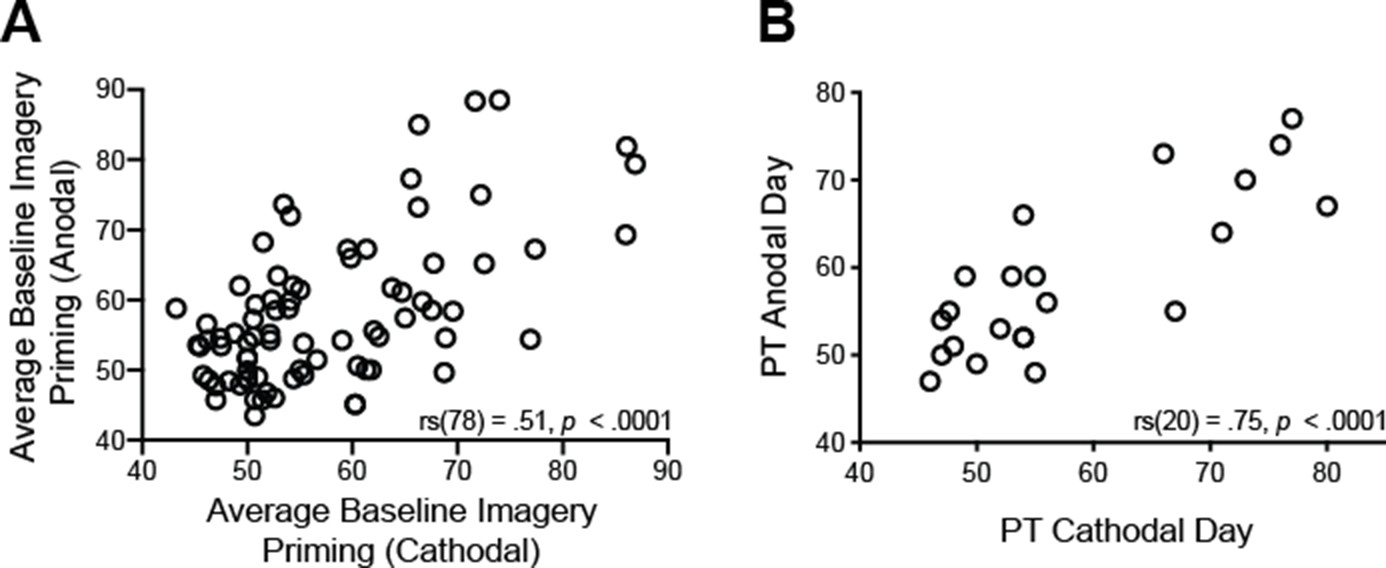
Re-test reliability for imagery strength (A) and Phosphene Thresholds (B).
(A) Scatterplot shows participants’ imagery strength measured by percent of binocular rivalry displays primed before tDCS stimulation across 2 days of testing (pre-anodal and pre-cathodal stimulation). Each data point represents one participant, 79 pairs in total. (B) Scatterplot shows participants’ 60% phosphene thresholds (PT) before tDCS stimulation across the 2 days of testing. Each data point represents one participant, 21 pairs in total.
Figure 2 with 3 supplements
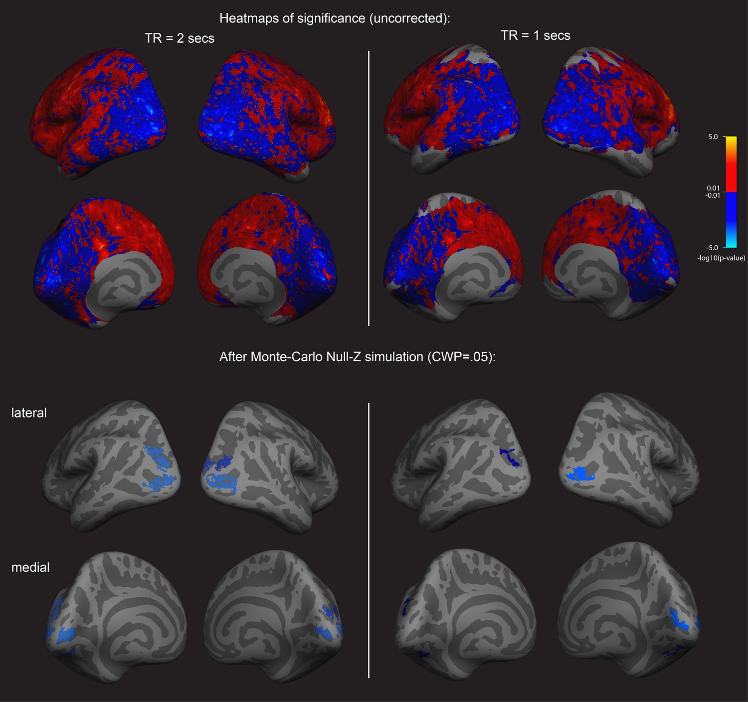
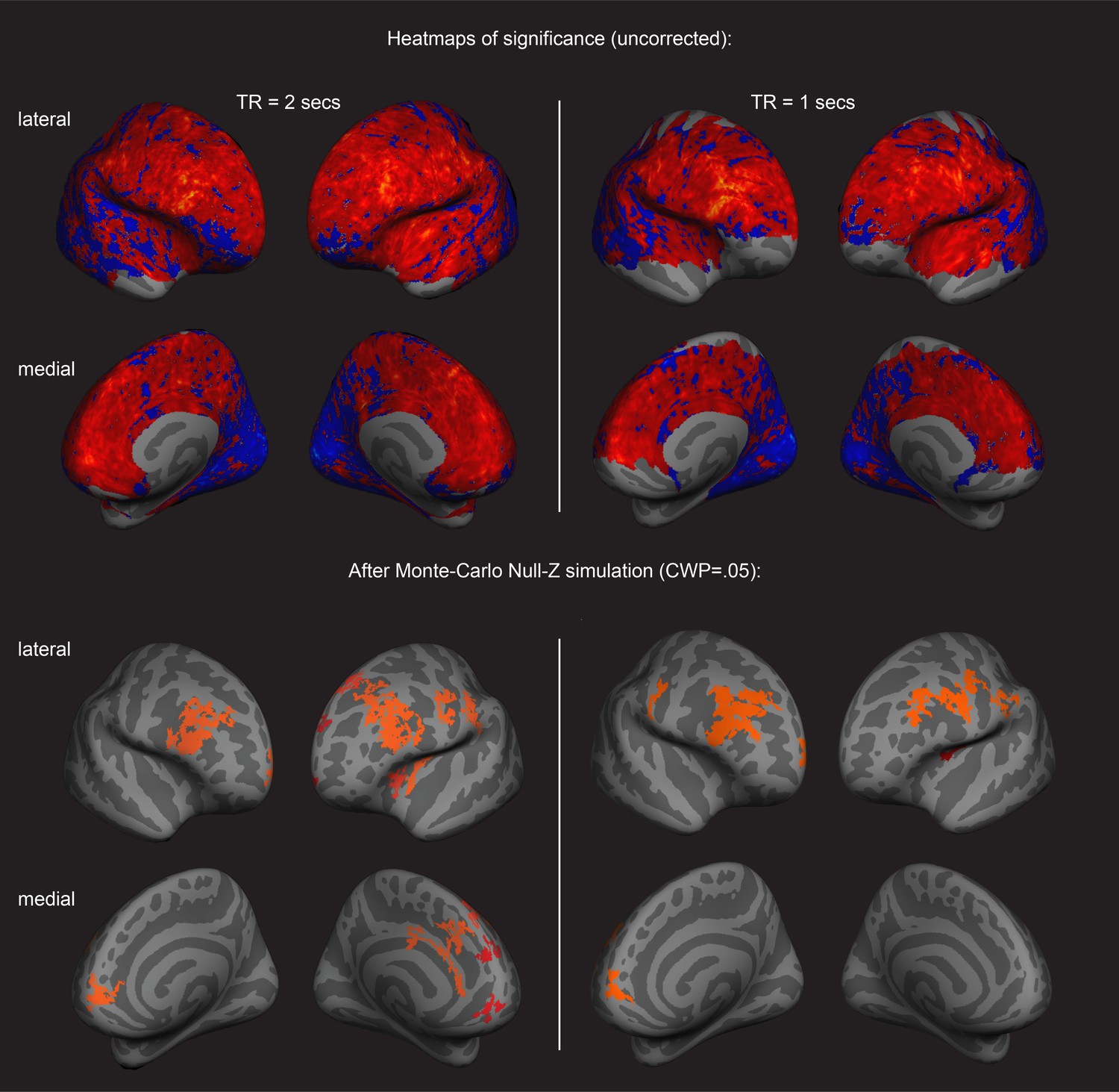
Surface-based whole brain analysis of data from two different fMRI resting-state measurements: negative associations with imagery strength in the occipital cortex.
Two columns on the left: results of the main resting-state fMRI data set with a TR of 2 s (TR2). Two columns on the right: results of an additional resting-state fMRI data set with a TR of 1 s (TR1); in those participants with which both measurements were conducted, about half were done on the same day. In the other half, the two measurements were conducted on different days. The two upper rows show the uncorrected (positive and negative) relationships with imagery as heatmaps. The two lower rows show the corrected clusters that had a negative association with individual imagery strength at a cluster-wise probability threshold (CWP) of p<0.05 (also see Supplementary file 1 - Supplementary Table S1). The two hemispheres are shown from the back, with the lateral view in the upper and the medial view in the lower panel. Multiple comparison correction was done using Monte Carlo Null-Z simulation (mc-z). No smoothing of the functional mean intensity data was applied. In line with the correlation analyses using normalised fMRI mean intensity of atlas- and retinotopically defined areas, only fMRI mean intensity clusters in the back of the brain, where early visual and lateral occipital cortex are located, showed negative associations with imagery strength (% primed). The fMRI measurement with a TR = 2 s has a better signal-to-noise ratio, as longer TR increase T2* tissue contrast (e.g. see Hashemi et al., 2010); in addition, the larger voxel size of the TR1 measurement (3.28 × 3.28×5 mm3) also means that they are more likely to pick up signals from other tissue (e.g. white matter), thereby increasing the contributions of biophysical noise. Both of this likely weakens the observed correlations with behavior; this might explain why none of the relationships with the brain areas using retinotopic mapping and the Desikan-Killiany atlas survived multiple comparison correction in the ROI-based approach (all p>0.05). Despite this, the clusters from the two different measurements in the surface-based group analysis show striking similarities; while the clusters in the TR1 measurement are smaller and sparser, their location in early visual and lateral occipital cortex are strongly overlapping with those found in the TR2 measurement. Further analyses showed that these similarities were not driven by the group that completed the measurements on the same day (analysis not shown).
Figure 2—figure supplement 1
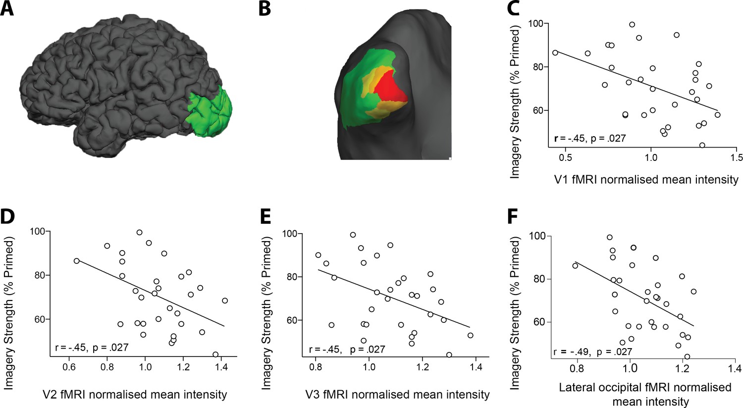
Retinotopic ROI anslysis of resting-state fMRI data and it's realtionship with imagery strength.
(A and B) Lateral view of the pial surface (A) and posterior view of the inflated surface (B) of the visual areas that showed a significant negative relationship with imagery. Red = V1, Orange = V2, Yellow = V3 and Green = lateral occipital area (C–F) Correlation between normalized mean fMRI intensity levels in V1, V2, V3, and lateral occipital area and imagery strength. Individuals with lower mean fMRI intensity levels in early visual cortex showed stronger imagery (FDR-corrected p-values to correct for multiple comparisons).
-
Figure 2—figure supplement 1—source data 1
fMRI resting state correlation data.
- https://cdn.elifesciences.org/articles/50232/elife-50232-fig2-figsupp1-data1-v1.csv
Figure 2—figure supplement 2
Surface-based brain analysis of data from two different fMRI resting-state measurements and imagery: positive associations with imagery strength in the frontal cortex.
Results of the main resting-state fMRI data set with a TR = 2 s are shown on the left (TR2); results of an additional resting-state fMRI data set with a TR = 1 s are shown on the right (TR1); in those participants with which both measurements were conducted, about half were done on the same day. In the other half, the two measurements were conducted on different days. The two upper rows show the uncorrected (positive and negative) relationships with imagery as heatmaps. The two lower rows show the corrected clusters that had a positive association with individual imagery strength at a cluster-wise probability threshold of p<0.05 (also see Supplementary Table S2). In both the lateral and medial views, the hemispheres are shown from the front. Multiple comparison correction was done using Monte Carlo Null-Z simulation (mc-z). No smoothing of the functional data was applied. In line with the correlation analyses using normalised fMRI mean intensity of atlas- and retinotopically defined areas, only fMRI mean intensity clusters in frontal areas showed positive associations with imagery strength (% primed). As elaborated in Figure 2, the signal-to-noise ratio is lower in the fMRI measurement with the TR of 1 s (on the right). In the ROI-based approach, none of the brain-behavior relationships survived multiple comparison correction (all p>0.05). Nevertheless, the clusters in the surface-based group analysis from the two different measurements show strong overlaps, indicating the reliability of the measurements. These similarities were not driven by the group that completed the measurements on the same day (analysis not shown).
Figure 2—figure supplement 3
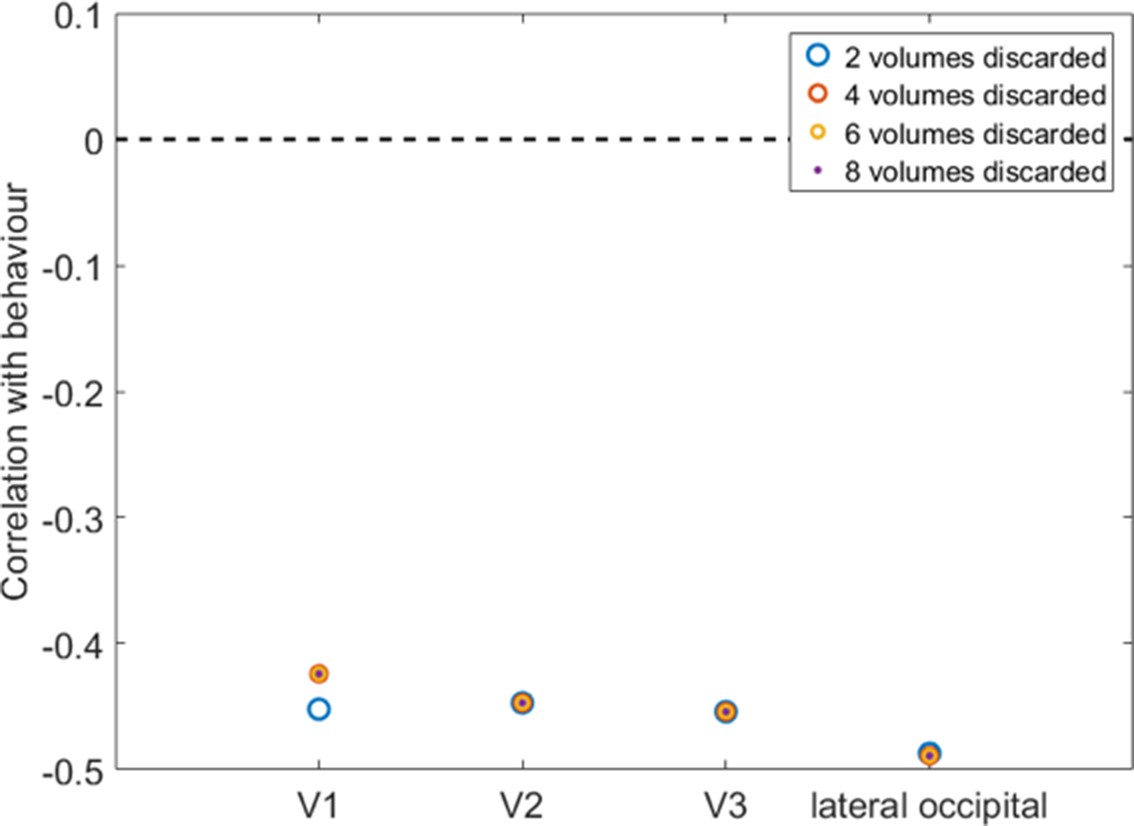
Visual cortex relationships with imagery strength and the number of EPI volumes discarded at the beginning of the run.
To allow for longitudinal magnetization equilibration to stabilize, it is standard to remove at least the first two (or more) volumes from the measurement. With a TR of 2 s, our analyses were conducted after exclusion of the first 2 volumes (blue mcircles). To ensure that this number was not too low, potentially causing the results to still be prone to magnetization artifacts, we re-analyzed the data after excluding 4 (red circles), 6 (yellow circles), and 8 volumes (purple circles). Irrespective of the number of discarded volumes at the beginning of the measurement, imagery strength correlations with visual cortices V1, V2, V3, and lateral occipital area remained almost identical.
Figure 3
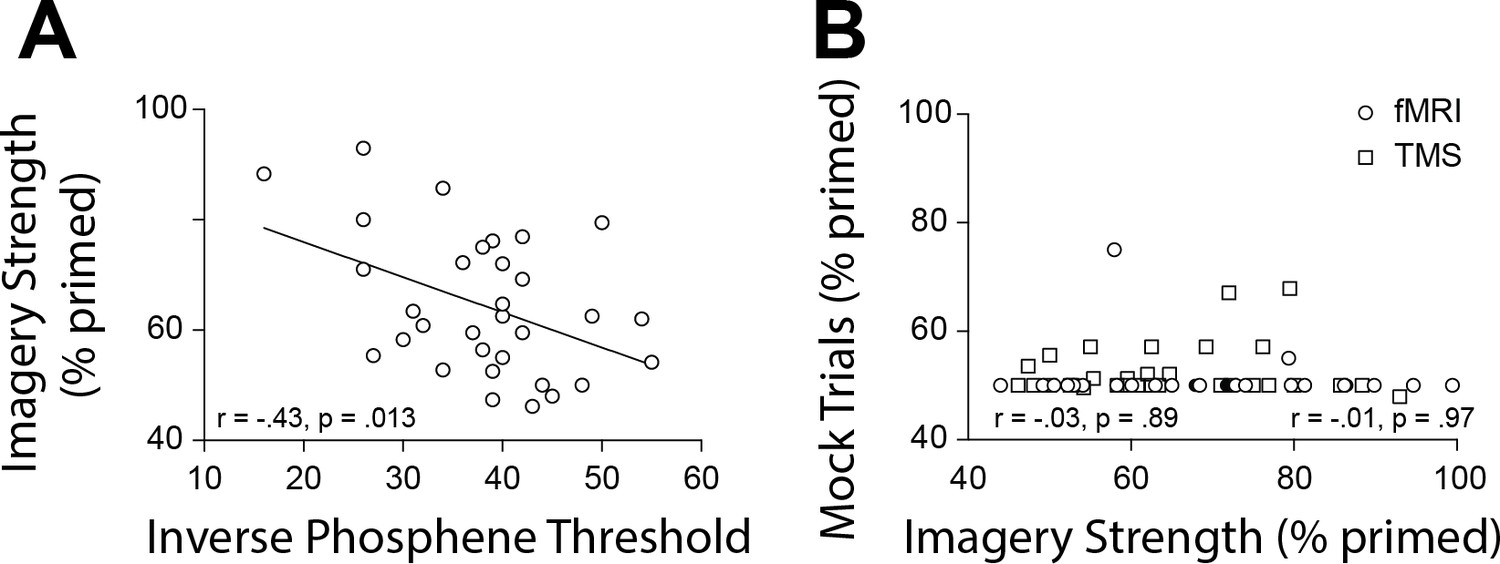
Scatterplots for TMS phosphene thresholds and mock rivalry data.
(A) Correlation between the inverse phosphene threshold and imagery strength. Individuals with lower cortical excitability in visual cortex tended to have stronger imagery. (B) Correlation between mock priming scores and real binocular rivalry priming for participants in the fMRI (circles) and TMS (squares) study. There was no significant association between perceptual priming in real and mock trials for the fMRI or TMS data. In the scatterplots (A & B), each data point indicates the value of one participant; the bivariate correlation coefficients are included with their respective significance levels.
-
Figure 3—source data 1
TMS inverse phosphene correlation data.
- https://cdn.elifesciences.org/articles/50232/elife-50232-fig3-data1-v1.csv
Figure 4 with 3 supplements
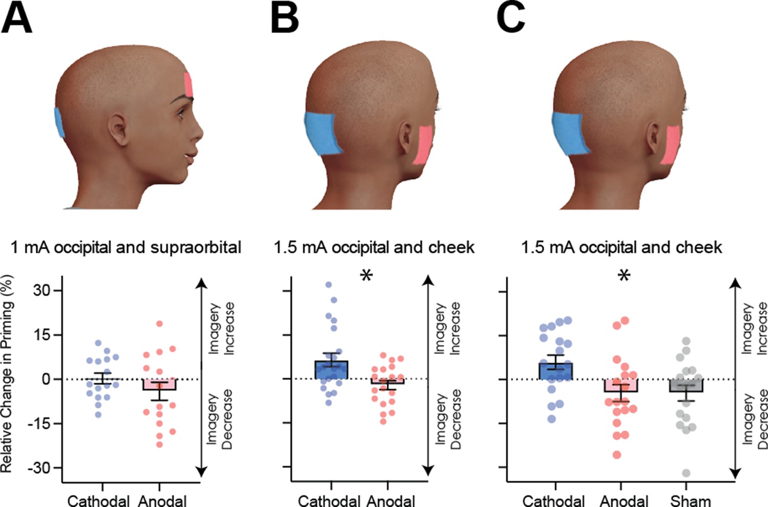
Visual cortex stimulation data.
(A) Effect of visual cortex stimulation on imagery strength at 1mA. The top image shows the tDCS montage, with the active electrode over Oz and the reference electrode on the supraorbital area. The bottom image shows the effect of cathodal (decreases excitability, blue dots represent each participant’s data) and anodal (increases excitability, red dots represent each individual participant’s data) stimulation averaged across all tDCS stimulation blocks (D1, D2, P1, and P2). (B) Effect of visual cortex stimulation on imagery strength at 1.5mA. Top: the tDCS montage with the active electrode over Oz and the reference electrode on the right cheek. Bottom: the effect of cathodal (blue dots, decrease excitability) and anodal (red dots, increase excitability) stimulation averaged across all blocks during and after tDCS stimulation (D1, D2, P1, and P2). Each data point represents a single participant. Imagery strength increases in the cathodal stimulation condition (blue), when neural excitability is reduced. (C) Effect of visual cortex stimulation on imagery strength at 1.5mA. Top: the tDCS montage with the active electrode over Oz and the reference electrode on the right cheek. Bottom: The left bar shows the relative change in imagery strength for cathodal stimulation (blue bar, blue dots represent individual participants data), the middle bar shows the relative change in imagery strength for anodal stimulation (red bar, red dots represent individual participants data), while the right bar shows the change in imagery strength for sham stimulation (grey bar, grey dots represent individual participants data). All error bars show ± SEMs and stars (*) indicate a significant effect of tDCS polarity.
-
Figure 4—source data 1
1mA occipital tDCS data.
- https://cdn.elifesciences.org/articles/50232/elife-50232-fig4-data1-v1.csv
-
Figure 4—source data 2
1.5mA occipital tDCS data.
- https://cdn.elifesciences.org/articles/50232/elife-50232-fig4-data2-v1.csv
-
Figure 4—source data 3
1.5mA occipital and sham tDCS data.
- https://cdn.elifesciences.org/articles/50232/elife-50232-fig4-data3-v1.csv
-
Figure 4—source data 4
1.5mA occipital TMS + tDCS data.
- https://cdn.elifesciences.org/articles/50232/elife-50232-fig4-data4-v1.csv
Figure 4—figure supplement 1

Raw tDCS imagery strength and difference scores as a function of block for experiments 1, 2 and 4.
(A) Experimental timeline for all tDCS experiments. Spread of individual data points for raw data and difference scores for experiment 1 (1mA Occipital: B and C), experiment 2 (1.5mA Occipital: D and E) and experiment 4 (1.5mA PreFrontal: F and G). Blue data points represent individual subjects’ cathodal stimulation changes while red data points represent anodal stimulation changes. For the raw data (B, D and F) the figure shows data averaged across pre, during and post-stimulation blocks. For the difference scores data (C, E and G) the figure shows difference scores for each imagery block, two during (D1 and D2, shaded yellow area) and two after tDCS (P1 and P2). All error bars show ± SEMs.
Figure 4—figure supplement 2

Raw tDCS imagery strength and difference scores as a function of block for experiments 3 and 5.
(A) Experimental timeline for all tDCS experiments. Spread of individual data points for raw data and difference scores for experiment 3 (Occipital stimulation: B and D), experiment 5 (Occipital + Prefrontal stimulation: C and E). For B and C blue data points represent individual subjects’ cathodal stimulation changes, red data points represent anodal stimulation changes and grey data points represent sham stimulation. For D and E blue data points represent cathodal-occipital and anodal-prefrontal stimulation, while blue represents anodal-occipital and cathodal-prefrontal stimulation, and grey data points represent sham stimulation. For the raw data (B and C) the figure shows data averaged across pre, during and post-stimulation blocks. For the difference scores (percent change) data (D and E), the figure shows difference scores (percent change) for each imagery block, two during (D1 and D2, shaded yellow area) and two after tDCS (P1 and P2). All error bars show ± SEMs.
Figure 4—figure supplement 3
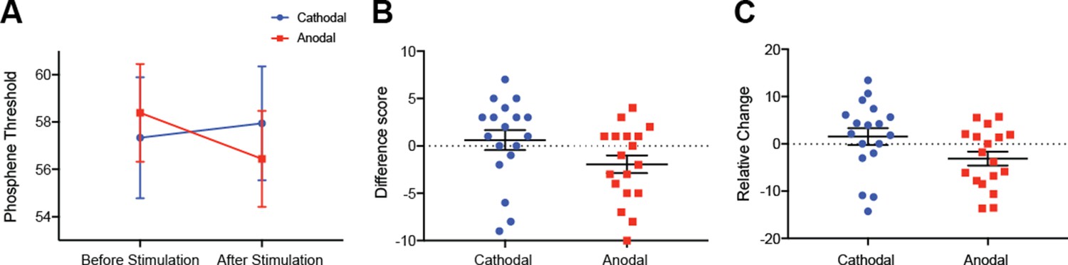
tDCS modulation of phosphene thresholds.
(A) Data shows phosphene thresholds (PT) before cathodal (left-hand side, blue data points) and before anodal (left-hand side, red data points) and after cathodal (right-hand side, blue data points) and after anodal stimulation (right-hand side, red data points). A significant interaction between tDCS polarity and PT session was found (F(1,17) = 6.16, p=0.02). (B) We then looked at the difference scores for each participant’s phosphene thresholds in the cathodal and anodal conditions. This difference score was calculated with the following equation: PT(after tDCS) – PT(before tDCS). Data shows participants’ phosphene threshold differences scores with positive scores indicating that PTs have increased after tDCS (in the cathodal condition, blue bar) while negative scores indicate that PTs have decreased after tDCS (in the anodal condition, red bar). There was a significant difference between the anodal and cathodal conditions with anodal PT changes being significantly lower than cathodal (t(17) = 2.48, p=0.02). (C) To assess whether or not some participants were driving these results, for example it might be that participants with high phosphene thresholds are driving the results, relative difference scores were also calculated: ((PT(after tDCS) – PT(before tDCS))/PT(before tDCS))*100. Using this method of analysis, the same pattern of results was found with cathodal stimulation increasing phosphene thresholds in comparison to anodal stimulation (t(17) = 2.70, p=0.015). All error bars show ± SEMs.
Figure 5
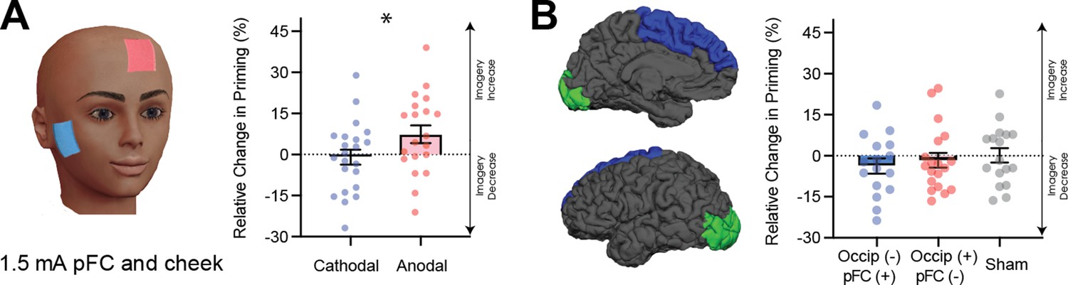
Data for prefrontal cortex stimulation.
(A) Effect of left prefrontal (pFC) cortex stimulation on imagery strength at 1.5mA. The left image shows the tDCS montage, with the active electrode between Fz and F3 and the reference electrode on the right cheek. The right image shows the effect of cathodal (decrease excitability, blue dots represent each participant’s difference score) and anodal (increase excitability, red dots represent each individual participant’s difference score) stimulation averaged across all blocks during and after tDCS stimulation (D1, D2, P1, and P2). Imagery strength can be seen to increase with anodal stimulation. (B) Effect of joint electrical stimulation of prefrontal cortex and visual cortex. The left image shows brain areas targeted in the final tDCS study. Data shows non-significant effects of cathodal occipital + anodal pFC stimulation (blue bars, blue dots represent individual participants data), anodal occipital + cathodal pFC stimulation (red bars, red dots represents individual participants data) and sham stimulation (grey bars grey dots represent individual participants data). All error bars show ± SEMs and stars (*) indicate a significant effect of tDCS polarity.
-
Figure 5—source data 1
1.5mA Prefrontal tDCS data.
- https://cdn.elifesciences.org/articles/50232/elife-50232-fig5-data1-v1.csv
-
Figure 5—source data 2
1.5mA combined tDCS data.
- https://cdn.elifesciences.org/articles/50232/elife-50232-fig5-data2-v1.csv
Tables
Table 1
Summary of montage, intensity, duration, and significance of each tDCS experiment.
| Experiment # | Montage (EEG Coordinates) | Intensity + duration | Notes | Significant |
|---|---|---|---|---|
| 1 Occipital | Active: Inion (Oz) Reference: Supraorbital (Fpz) | 1 mA 15 min | Tested effect on imagery strength | ✗ |
| 2 Occipital | Active: Inion (Oz) Reference: Right Cheek | 1.5 mA 15 min | Tested effect on imagery strength | ✓ |
| 3 Occipital | Active: Inion (Oz) Reference: Right Cheek | 1.5 mA 15 min | Tested effect on imagery strength (additional sham condition) | ✓ |
| 4 Prefrontal | Active: Between F3-Fz Reference: Right Cheek | 1.5 mA 15 min | Tested effect on imagery strength | ✓ |
| 5 Occipital + Prefrontal | Active: Inion (Oz) Active: Between F3-Fz | 1.5 mA 15 min | Tested effect on imagery strength | ✗ |
| Additional control Occipital | Active: Inion (Oz) Reference: Right Cheek | 1.5 mA 15 min | Tested effect on phosphene threshold | ✓ |
Table 2
Exclusion criteria for tDCS experiments.
| Exclusion | Explanation |
|---|---|
| Mock Priming (Higher than 66%) | Mock displays are fake binocular rivalry displays – priming on these trials indicates that participants are showing a response/demand characteristic and as such we cannot trust their priming scores, as they may either be responding in a way that they think we want them too, or they are not attending to the task correctly. A score of more than 66% indicates that the participant has primed on these mock trials more than once. |
| Low Priming (lower than 40%) | Participants whose imagery scores were lower than 40% were excluded, as the score becomes difficult to interpret: The measure of imagery strength is predicated on how the energy of a stimulus impacts on binocular rivalry. Very weak perceptual stimuli prime binocular rivalry up unto a certain point. At this tipping point, as the image becomes stronger, it begins to suppress binocular rivalry (Brascamp et al., 2007). For this reason, very low priming can either mean that the participant’s visual imagery is so strong that it leads to suppression, or that the opposite is the case, and imagery is in fact very weak. Alternatively, it may also be that a participant is not completing the task correctly. 40% was chosen as the cut off as this is 10% lower than chance values (50%). |
| Mixed Percepts (higher than 1/3 or 33%) | We analyse our priming data as percent primed,that is the percentage of trials a participant imagined an image, then saw that image in the following display. Mixed trials cannot be labelled as either ‘primed’ or ‘not primed’, and as such these trials are not included in the analysis. A high number of mixed trials reduces the number of usable trials for analysis. This can lead to large changes that may be spurious (much larger percentage changes due to a single trial) and not due to the stimulation parameters. We excluded an individual’s data set if more than a third of the trials were mixed percept’s. |
| Attrition | Attrition occurred when a participant did not turn up to or cancelled the second and/or third day of testing. |
| Impedance (Exceeding voltage: impedance greater than 55 kΩ) | For safety reasons, our tDCS machine was programmed to shut off once the impedance exceeded 55 kΩ (this is pre-programmed into the tDCS machine). As the participants completed the experiment in a blackened room by themselves we could not monitor the impedance of the machine in real-time and as such the machine could switch off during a block of the experiment. As we cannot know how much stimulation this participant received we are unable to use them reliably in our analysis – as different stimulation durations will lead to different excitability changes. The second (1.5mA Occip + cheek) and fourth (1.5mA pFC + cheek) tDCS experiments were run at the same time. There were a large number of cases of impedance being exceeded in these studies – it was discovered that this was due to a faulty wire, which was replaced halfway through the experimental data collection. |
| Phosphene Determination | If participants reported phosphenes in the wrong visual hemifield (e.g. left visual hemisphere was stimulated and participants reported phosphenes in the left visual hemifield) their data was excluded. Participants who had very large eye-blinks in the REPT procedure were excluded from the experiment, due to this potentially resulting in a missed phosphene leading to incorrect phosphene threshold estimation. |
Table 3
Number of participants excluded per exclusion criteria for tDCS experiments.
| Exclusion criteria | Exp 1 | Exp 2 | Exp 3 | Exp 4 | Exp 5 | Exp 6 | Total |
|---|---|---|---|---|---|---|---|
| Mock priming | 1 | 2 | 2 | 5 | |||
| Low priming | 2 | 2 | 1 | 3 | 8 | ||
| Mixed percept’s | 3 | 2 | 1 | 6 | |||
| Attrition | 1 | 1 | |||||
| Impedance | 9 | 4 | 1 | 2 | 16 | ||
| Incorrect buttons | 1 | 3 | 4 | ||||
| Technical issues | 3 | 2 | 5 | ||||
| Phosphenes | 6 | 6 | |||||
| Total | 5 | 13 | 6 | 7 | 9 | 11 | 51 |
Additional files
-
Source code 1
LME code for r analysis.
- https://cdn.elifesciences.org/articles/50232/elife-50232-code1-v1.rtf
-
Supplementary file 1
fMRI tables.
- https://cdn.elifesciences.org/articles/50232/elife-50232-supp1-v1.docx
-
Transparent reporting form
- https://cdn.elifesciences.org/articles/50232/elife-50232-transrepform-v1.docx
Download links
A two-part list of links to download the article, or parts of the article, in various formats.
Downloads (link to download the article as PDF)
Open citations (links to open the citations from this article in various online reference manager services)
Cite this article (links to download the citations from this article in formats compatible with various reference manager tools)
Cortical excitability controls the strength of mental imagery
eLife 9:e50232.
https://doi.org/10.7554/eLife.50232


