The sifting of visual information in the superior colliculus
- Division of Biology and Biological Engineering, California Institute of Technology, United States
Figures
Figure 1 with 1 supplement

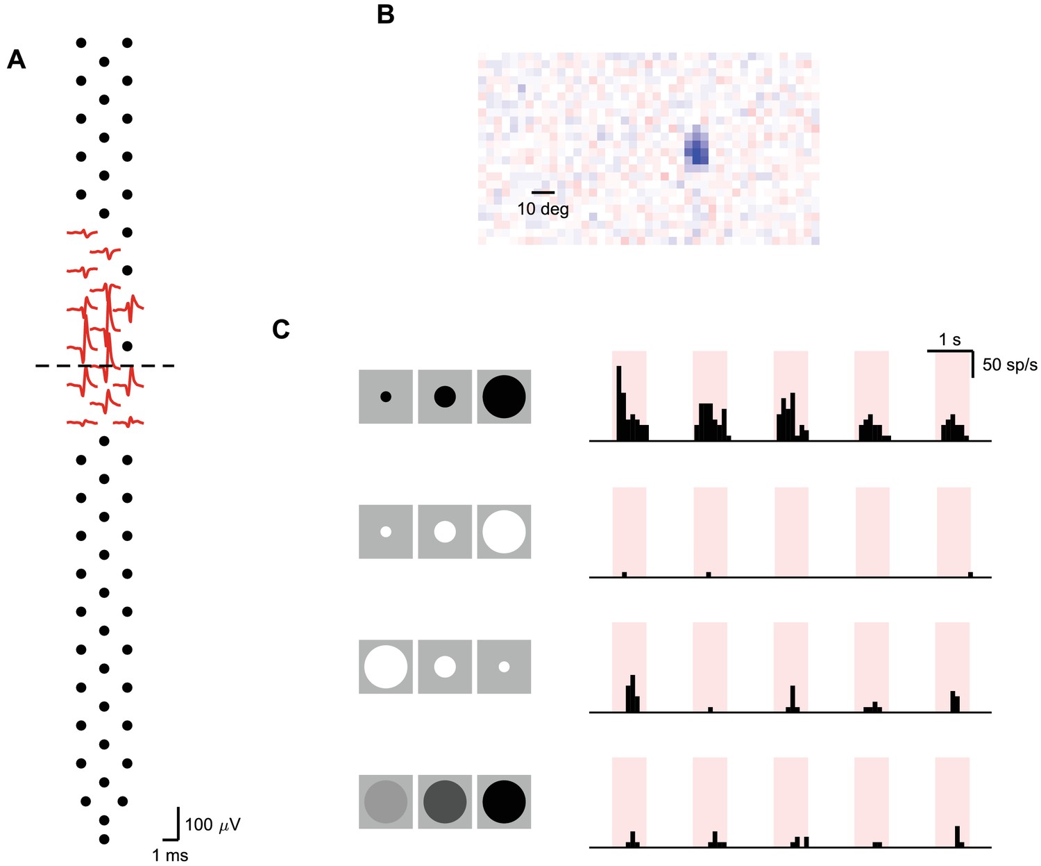
The emergence of selectivity, invariance, and stimulus-specific habituation along the depth of SC.
(A) Left: Experimental setup. Silicon neural probes with 128 channels were implanted into the SC of a headfixed mouse viewing visual stimuli. The mouse was free to run on a circular treadmill. Middle: Diagram of a coronal section showing the anatomically defined layers of the SC (adapted from Paxinos and Franklin, 2001). sSC: superficial SC; dSC: deep SC. Right: Corresponding histological section recovered after neural recording, showing tracks of two electrode prongs. Magenta: DiI; white: anti-Calb1. (B) Extracellular spike waveforms of sample sSC (red) and dSC (blue) neurons recorded simultaneously on the silicon probe. Dots indicate the location of recording sites. Dashed line indicates boundary along the electrode array between sSC and dSC (see Materials and methods and Figure 1—figure supplement 1). (C) Response of neurons from (B) to visual stimuli. The sSC neuron (middle) responds to many types of figural stimuli (left icons: expanding black, expanding white, contracting black, contracting white, dimming, and moving black disk), whereas the dSC neuron (right) is highly selective to the expanding black disk. The sSC neuron responds robustly to every trial, whereas the dSC neuron responds primarily to the first presentation. (D) In an experiment in which looming stimuli appear from many locations (left), the sSC neuron from (B) (middle) is driven only by stimuli that cross its receptive field, whereas the dSC neuron from (B) (right) responds to stimuli placed at many more locations. White: final size of looming stimuli that elicited significant response from the cell; red: one standard deviation outline of spatial receptive field recovered by spike-triggered average method.
Figure 1—figure supplement 1
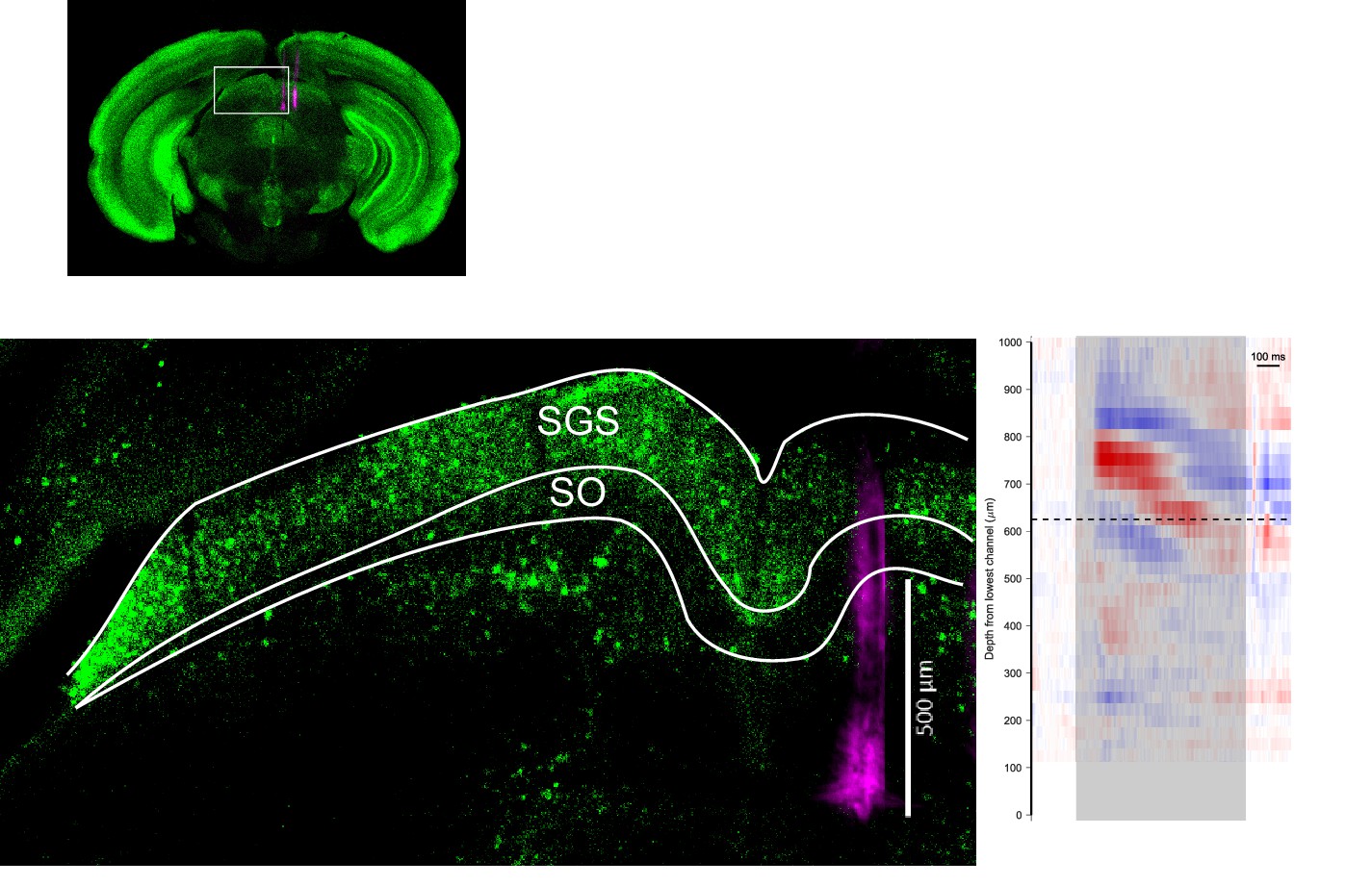
Histological and electrophysiological identification of SC layers.
(Top) Brain section (coronal, 100 µm thick) showing the recorded area from an experiment. (Bottom left) Boxed area in the top panel is enlarged. The probe track is marked with DiI (magenta). The anti-Calb1 antibody (green) stains superficial gray layer (SGS) and upper parts of the intermediate gray layer but does not stain the optic layer (SO). White lines mark the top and bottom outline of the SGS and SO. (Bottom right) Current source density analysis of the same recording displayed at the same spatial scale as the section on the left. Looming stimulus was delivered during the time window shaded in gray. Dashed line marks the inflection point that separates current sink (blue) below and current source (red) above. This corresponds to the lowermost point of SGS, as previously reported by Stitt et al. (2013).
Figure 2 with 1 supplement
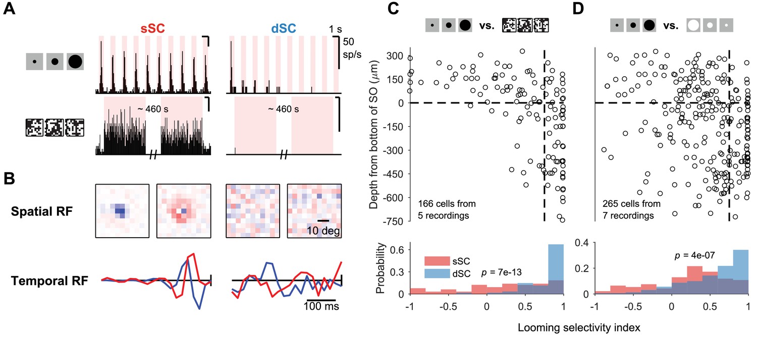
Selectivity to looming stimulus.
(A) Response of sample sSC (middle) and dSC (right) neurons to looming stimulus (top) and flickering checkerboard (bottom). sSC neuron is driven strongly by both, but dSC neuron is almost completely silent to the checkerboard stimulus. (B) Spatial (top) and temporal (bottom) receptive fields of the sSC (left) and dSC (right) neurons in (A) based on spike-triggered average analysis. In each subpanel, left: spatial center; right: spatial surround; bottom blue: temporal center; bottom red: temporal surround. In the temporal RF panels, the vertical line represents the time of the spike. (C) Population summary of selectivity to looming stimulus over checkerboard stimulus along the depth of SC. Horizontal dashed line indicates the boundary between sSC and dSC. Vertical dashed line separates neurons with high selectivity index (>0.75) from others. The p-value (two-sample Kolmogorov-Smirnov test) indicates that the distributions of sSC and dSC neurons differ significantly. (D) Same as (C), comparing responses to looming stimulus and contracting white disk. Selectivity index is defined as where refers to response to looming stimulus and refers to response to checkerboard stimulus (C) or contracting white disk (D).
Figure 2—figure supplement 1
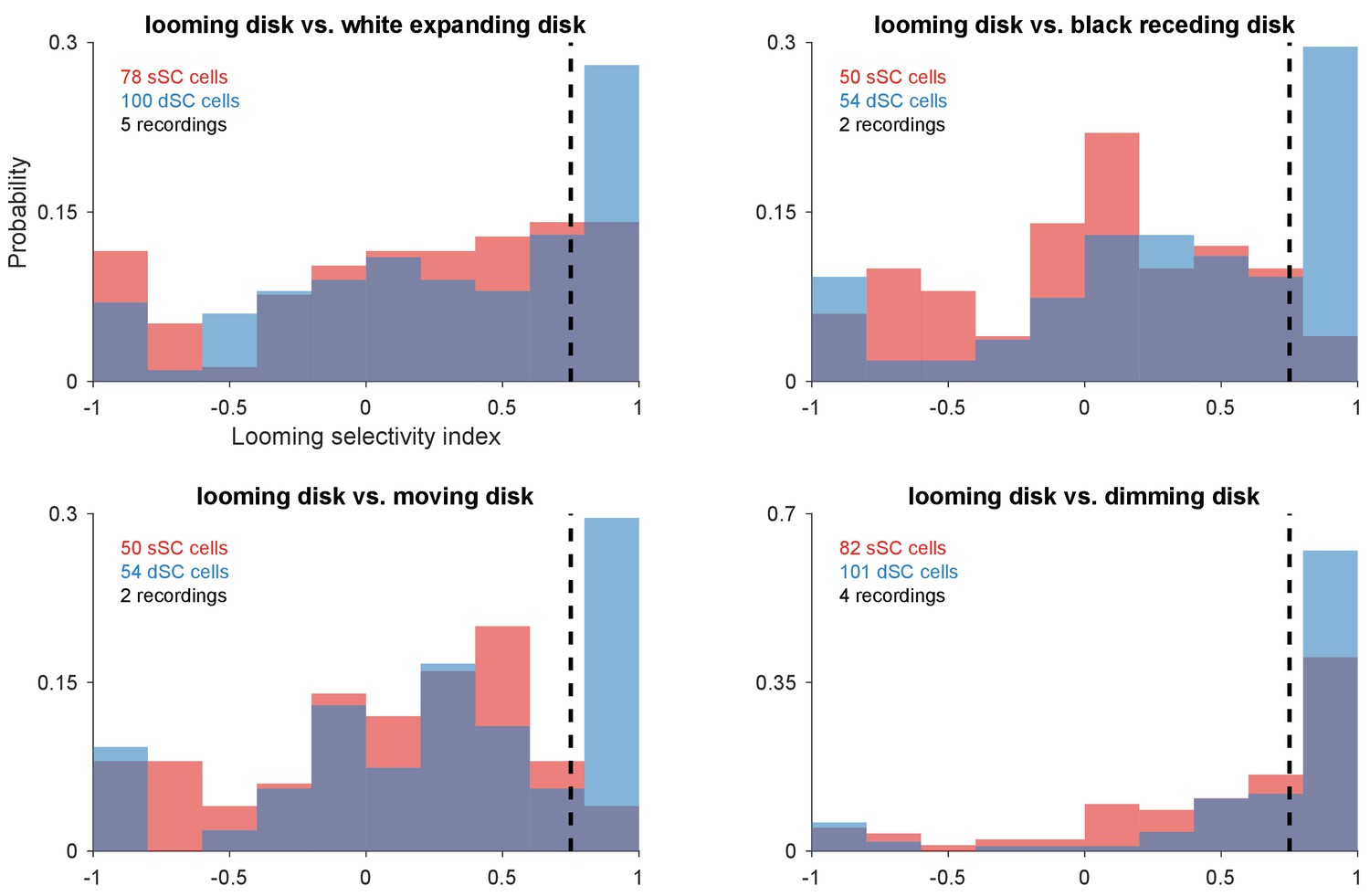
Looming selectivity over other figural stimuli.
Distribution of looming selectivity index for neurons in the superficial and deep SC vs. expanding white disk, receding dark disk, moving disk, and dimming disk. Dotted line separates neurons with high looming selectivity index (>0.75) from others.
Figure 3
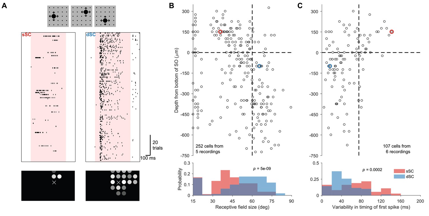
Invariance to stimulus position.
(A) Raster plot of sample sSC (left) and dSC (right) neurons recorded simultaneously during an experiment in which looming stimuli appear randomly in one of 25 locations (small black dots in cartoon) in each trial. These locations are ∼15°apart. The dSC neuron responds to many more locations than the sSC neuron and with an invariant latency. Bottom: The response amplitude at each location is reported by the brightness of the circle. X indicates a location that received no stimulus. (B) Population summary of receptive field size estimated from the experiment in (A). Vertical dashed line is at 60°. (C) Population summary of variability in the timing of the first spike from the experiment in (A). Vertical dashed line is at 75 ms. In both (B) and (C), the horizontal dashed line separates sSC and dSC. The red and blue circles denote the sSC and dSC neurons from (A). The -values (two-sample Kolmogorov-Smirnov test) indicate that the distributions of sSC and dSC neurons differ significantly.
Figure 4 with 3 supplements
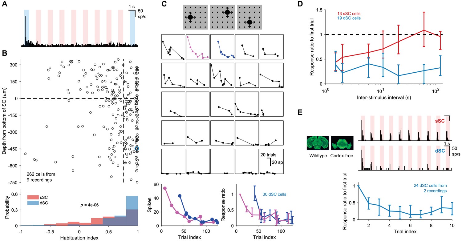
Stimulus-specific habituation.
(A) Response of a sample dSC neuron to a series of 10 looming stimuli. The first and the 10th trials are shaded in blue. Note that this neuron has a maintained baseline firing rate, which is unchanged by the stimulus on all but the first trial. (B) Population summary of habituation to repeated looming stimulus. The habituation index is defined as where refers to the number of spikes fired in in i-th trial after subtracting background activity. The horizontal dashed line separates sSC and dSC. The vertical dashed line is at 0.75. The blue circle is the sample dSC neuron from (A). The p-value (two-sample Kolmogorov-Smirnov test) indicates that the distributions of sSC and dSC differ significantly from each other. (C) Response of a sample dSC neuron to ~100 presentation of looming stimuli delivered in random sequence. Each subpanel represents response to stimuli at one of the 25 locations. Bottom left: two of the response traces from above. Even after the neuron has habituated to stimuli at one location (magenta), it responds strongly to the first stimulus at another location (blue). Bottom right: response of all dSC neurons in this recording, normalized by response to first trial of the magenta trace. Data points are medians and error bars range from 25th to 75th percentiles. (D) Summary of time to recover from habituation for a group of simultaneously recorded sSC and dSC neurons. Even after ~120 s, dSC neurons do not recover beyond 50% of the initial response. Data points are medians and error bars range from 25th to 75th percentiles. (E) Sample sSC (top right) and dSC (middle right) neurons recorded in a mutant mouse that does not develop the neocortex or the hippocampus (left). The dSC neuron in the mutant mouse also shows habituation. Bottom: population response of dSC neurons to 10 presentations of the looming stimulus, normalized by the response to the first presentation. Data points are medians and error bars range from 25th to 75th percentiles.
Figure 4—figure supplement 1
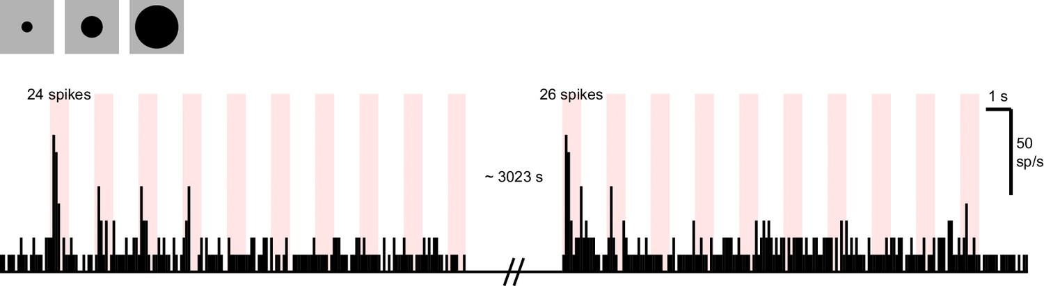
Suppression of a familiar stimulus is not permanent.
The response of a sample dSC neuron to looming stimuli that were presented in the beginning (left) and the end (right) of a recording. Other stimuli (e.g. checkerboard) were presented to the animal in the ~50 min that separates these two blocks. Note that this neuron eventually does recover (24 vs. 26 spikes to the first presentation), indicating that the memory of looming stimulus is not permanent.
Figure 4—figure supplement 2
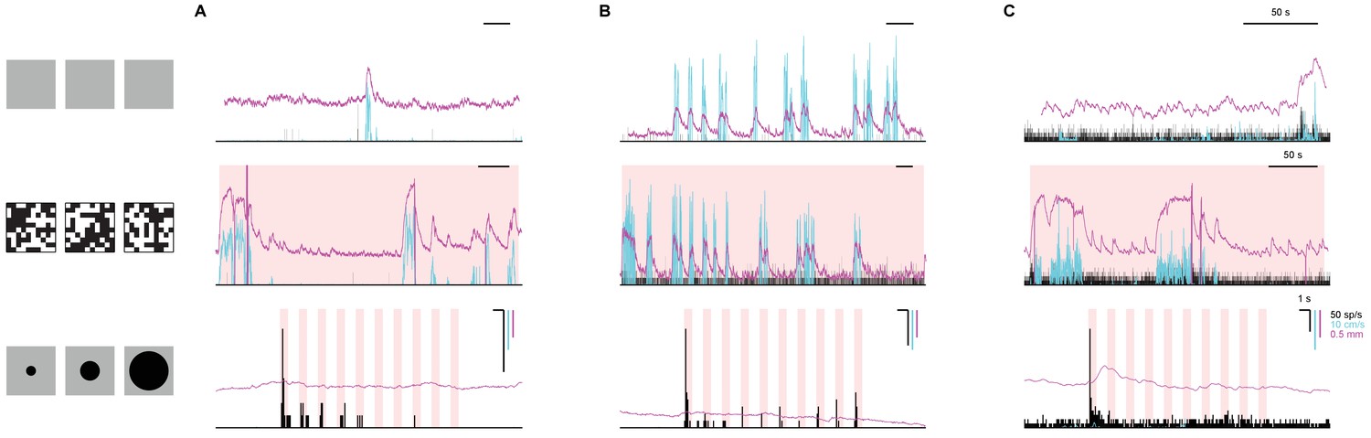
Enhanced response to first stimulus is not a simple consequence of motor activity.
The response of three sample dSC neurons from Figure 1 (A), Figure 3A (B), and Figure 4A (C) to no stimulus (top), checkerboard stimulus (middle), and looming stimulus (bottom) are shown, along with simultaneously recorded locomotion (cyan) and pupil diameter (magenta). The neurons are silent during no stimulus and checkerboard stimulus even though the locomotion and pupil size are modulated. This suggests that the strong response in the first presentation of the looming stimulus is not simply a result of motor output or change in arousal level in the absence of visual threat. In one case (C, bottom), the burst of firing to the looming stimulus precedes a significant change in the pupil size, suggesting an increased level of arousal.
Figure 4—figure supplement 3
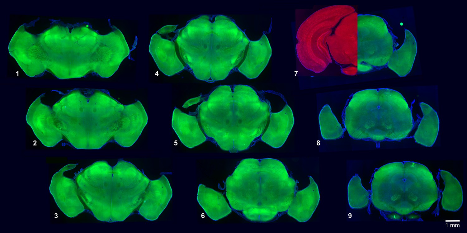
A mutant mouse that lacks the neocortex and the hippocampus.
A series of Emx1-Cre:Pals1flox/flox mouse brain coronal sections (100 µm thick), labeled from most anterior (1) to most posterior (9). The left half of panel seven shows a corresponding wild-type mouse coronal section with a fully developed neocortex and hippocampus. Note that these structures are lacking in the mutant mouse. Autofluorescence (green, red), DAPI (blue).
Figure 5
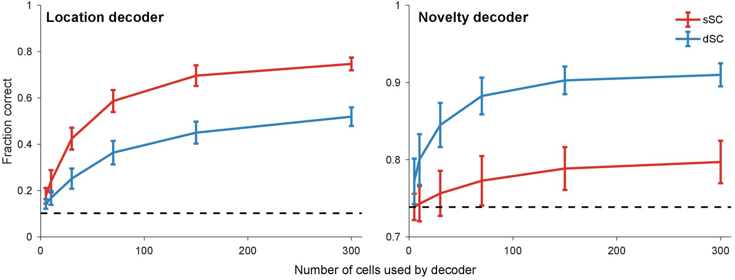
Population decoding of distinct stimulus features.
Linear decoders were trained with simultaneously recorded sSC and dSC neurons to predict location (left) and novelty (i.e. whether the stimulus has appeared at a location for the first time) (right) of stimuli in the experiment described in Figure 3. Dashed line: chance performance; error bars: one standard deviation across different subsamples of cells.
Figure 6 with 1 supplement
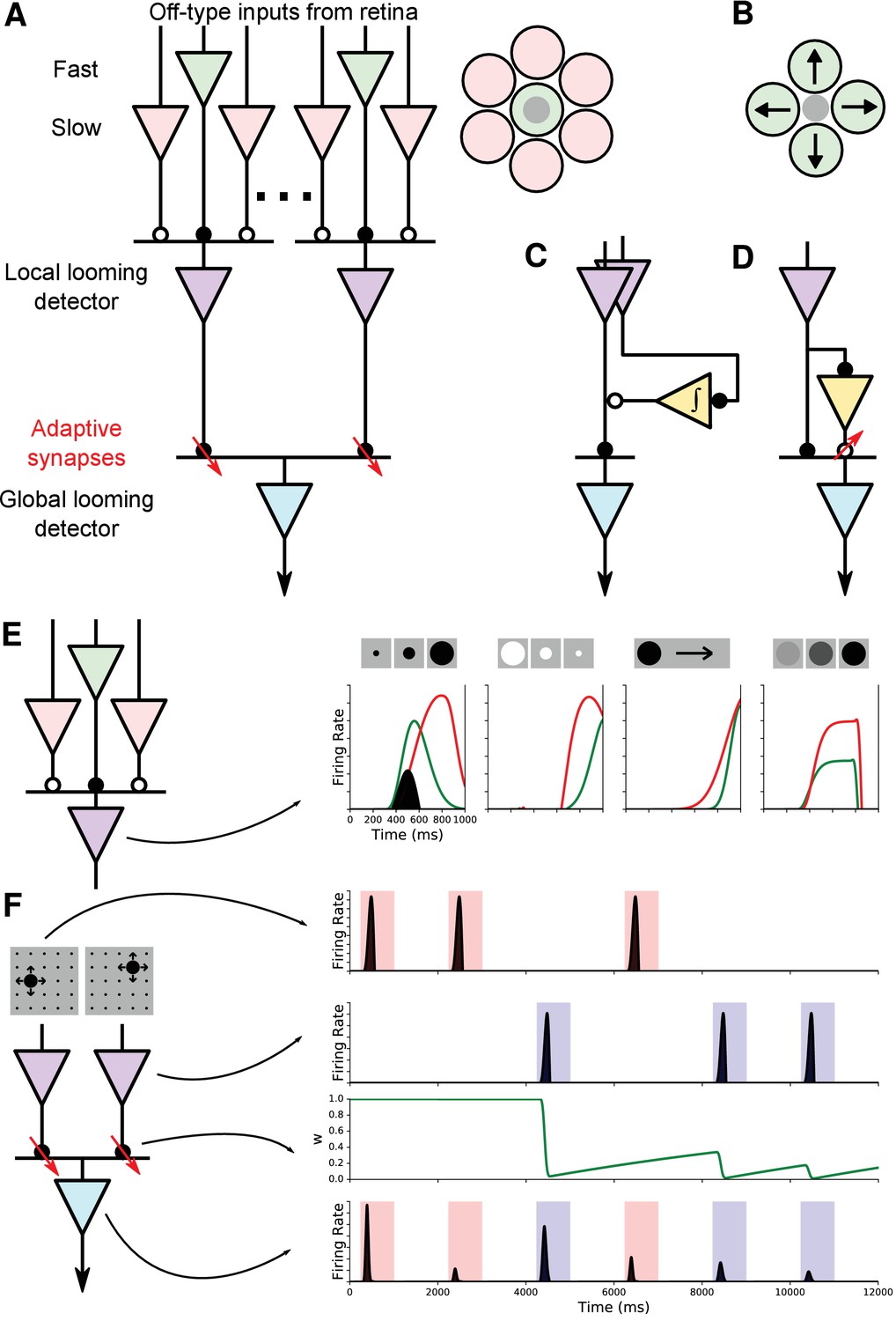
Model of selectivity, invariance, and stimulus-specific habituation.
(A) The ‘working model’ of how selectivity, invariance, and habituation arise in the dSC. Looming selectivity is generated by combining fast and slow Off-type retinal inputs (green and pink) in the local looming detector (purple) in sSC. Inset on right shows spatial layout of these inputs. Invariance arises from pooling these local looming detectors to a single global looming detector (cyan) in the deep layers. The stimulus-specific habituation is achieved by synapses that undergo activity-dependent short-term depression (red downward arrows). Solid circles: excitation; open circles: inhibition. (B) An alternative model of looming selectivity based on pooling directionally tuned inputs. (C, D) Alternative models of stimulus-specific habituation: the same input as the excitation drives a persistent inhibition (C) or a facilitating inhibitory synapse (D). (E) Simulation of responses to various figural stimuli. Green: excitation from center; red: inhibition from surround; shaded black: net response. (F) Simulation of stimulus-specific habituation. Each local looming detector connects to the global looming detector with a synapse whose strength decays rapidly and recovers slowly.
Figure 6—figure supplement 1
A putative local looming detector.
One of several putative local looming detector identified in the superficial SC (A), with a local receptive field (B) and selectivity for looming stimulus without a significant habituation to repeated stimuli (C). Dashed line: boundary between sSC and dSC.
Figure 7

The logic of selectivity and invariance.
In (A) feature selectivity is accomplished by combining local input signals (red and green) with AND logic (X). Then invariance arises from combining many of those feature signals with OR logic (+). In (B) there is only a single feature computation (X). Invariance is achieved by routing its inputs to local signals in different parts of the visual field. Arrows indicate where the stimulus-specific habituation must take place.
Tables
Table 1
Parameter values used for the model in Figure 6, as defined by Equations 3, 4, 5, 6, and 9.
| Receptive field (Equations 3, 4 and 5) | ||
|---|---|---|
| Parameter | Center | Surround |
| 4.00° | 10.0° | |
| 104 ms | 84.6ms | |
| 2.77 | 1.24 | |
| 91.2 ms | 79.7 ms | |
| 3.94 | 1.87 | |
| 1.34 | 1.33 | |
| Nonlinearity (Equation 6) | ||
| Parameter | Value | |
| 1 | ||
| 0 | ||
| Synaptic depression (Equation 9) | ||
| Parameter | Value | |
| 1 | ||
| 0 |
Additional files
Download links
A two-part list of links to download the article, or parts of the article, in various formats.
Downloads (link to download the article as PDF)
Open citations (links to open the citations from this article in various online reference manager services)
Cite this article (links to download the citations from this article in formats compatible with various reference manager tools)
The sifting of visual information in the superior colliculus
eLife 9:e50678.
https://doi.org/10.7554/eLife.50678


