Energy efficient synaptic plasticity
- School of Psychology, University of Nottingham, United Kingdom
- School of Mathematical Sciences, University of Nottingham, United Kingdom
Figures
Figure 1 with 1 supplement
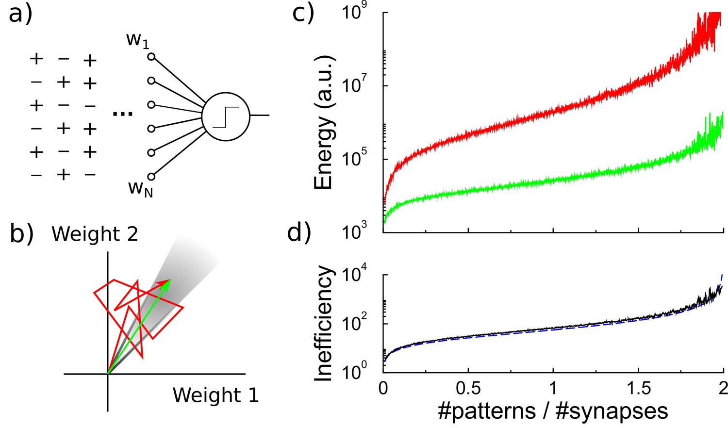
Energy efficiency of perceptron learning.
(a) A perceptron cycles through the patterns and updates its synaptic weights until all patterns produce their correct target output. (b) During learning the synaptic weights follow approximately a random walk (red path) until they find the solution (grey region). The energy consumed by the learning corresponds to the total length of the path (under the norm). (c) The energy required to train the perceptron diverges when storing many patterns (red curve). The minimal energy required to reach the correct weight configuration is shown for comparison (green curve). (d) The inefficiency, defined as the ratio between actual and minimal energy plotted in panel c, diverges as well (black curve). The overlapping blue curve corresponds to the theory, Equation 3 in the text.
Figure 1—figure supplement 1

Energy inefficiency as a function of exponent in the energy function.
The energy inefficiency of perceptron learning for various energy variants. The energy inefficiency of perceptron learning when the energy associated to synaptic update is and the exponent is varied (green curve). The case is used throughout the main text. The inefficiency is the ratio between the energy needed to train the perceptron and the energy required to set the weights directly to their final value. When , the energy is equal to the number of updates made. When , the energy is the sum of individual update amounts. When it costs less energy to make many small weight updates compared to one large one. When , this effect is so strong that even the random walk of the perceptron is less costly than directly setting the weights to their final value. We consider to be the biologically relevant regime. Also shown is the inefficiency when only potentiation costs energy, and depression comes at no cost that is (overlapping cyan curve). This has virtually identical (in)efficiency.
Figure 2 with 1 supplement
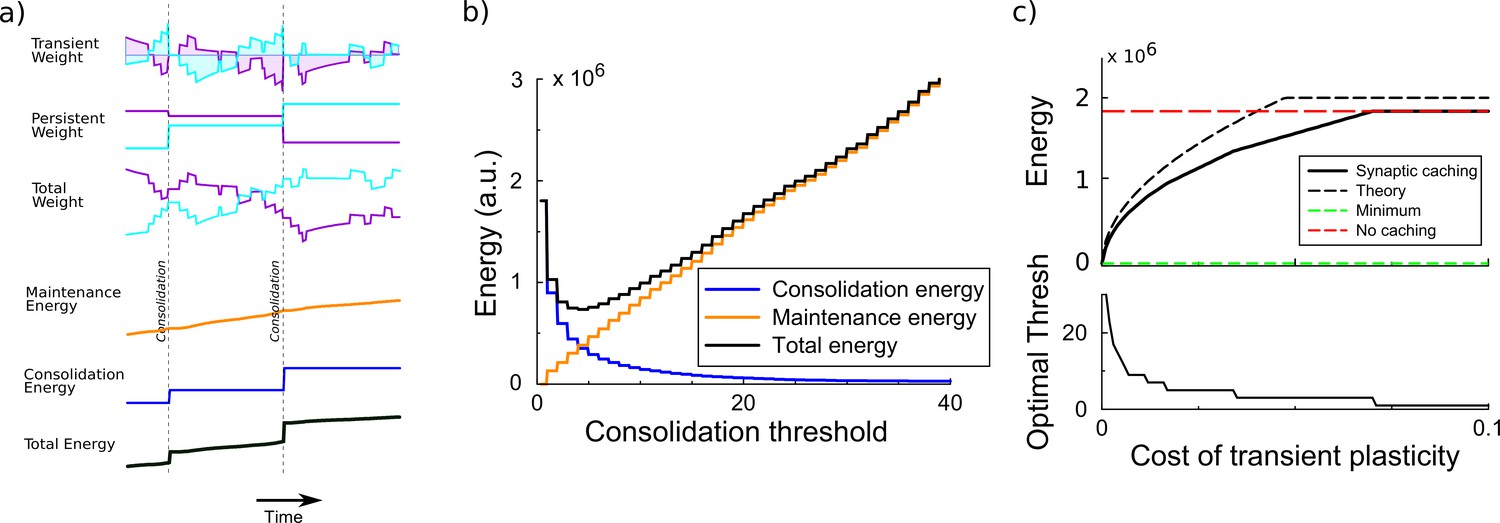
Synaptic caching algorithm.
(a) Changes in the synaptic weights are initially stored in metabolically cheaper transient decaying weights. Here, two example weight traces are shown (blue and magenta). The total synaptic weight is composed of transient and persistent forms. Whenever any of the transient weights exceed the consolidation threshold, the weights become persistent and the transient values are reset (vertical dashed line). The corresponding energy consumed during the learning process consists of two terms: the energy cost of maintenance is assumed to be proportional to the magnitude of the transient weight (shaded area in top traces); energy cost for consolidation is incurred at consolidation events. (b) The total energy is composed of the energy to occasionally consolidate and the energy to support transient plasticity. Here, it is minimal for an intermediate consolidation threshold. (c) The amount of energy required for learning with synaptic caching, in the absence of decay of the transient weights (black curve). When there is no decay and no maintenance cost, the energy equals the minimal one (green line) and the efficiency gain is maximal. As the maintenance cost increases, the optimal consolidation threshold decreases (lower panel) and the total energy required increases, until no efficiency is gained at all by synaptic caching.
Figure 2—figure supplement 1

Synaptic caching in a spiking neuron with a biologically plausible perceptron-like learning rule.
To demonstrate the generality of our results, independent of learning rule or implementation, we implement a spiking biophysical perceptron. D'Souza et al. (2010) proposed perceptron-like learning by combining synaptic spike-time dependent plasticity (STDP) with spike-frequency adaptation (SFA). In their model, the leaky integrate-and-fire neuron receives auditory input and delayed visual input. The neuron’s objective is to balance its auditory response to its visual response by adjusting the weights of its auditory synapses through STDP. The visual input is the supervisory signal. We use 100 auditory inputs, and measure the energy for the neuron to learn so that each auditory input pattern becomes associated to a (binary) visual input. We repeatedly present patterns , each with two activated auditory inputs until stabilized as D’Souza et al. The training is considered successful if the auditory responses of all the input patterns associated to the same binary visual input fall within two standard deviations from the mean auditory response of those patterns, and are at least five standard deviations away from the mean auditory response of other patterns. Synaptic caching is implemented as in the main text by splitting into persistent forms and transient forms. We consider the optimal scenario where the transient weights do not decay and have no maintenance cost. Also in the biophysical implementation of perceptron learning, synaptic caching (green curve) saves a significant amount of energy compared to without caching (red curve), suggesting that synaptic caching works universally regardless of learning algorithm or biophysical implementation.
Figure 3 with 1 supplement

Synaptic caching and decaying transient plasticity.
The amount of energy required, the optimal consolidation threshold, and the learning time as a function of the decay rate of transient plasticity for various values of the maintenance cost. Broadly, stronger decay will increase the energy required and hence reduce efficiency. With weak decay and small maintenance cost, the most energy-saving strategy is to accumulate as many changes in the transient forms as possible, thus increasing the learning time (darker curves). However, when maintenance cost is high, it is optimal to reduce the threshold and hence learning time. Dashed lines denote the results without synaptic caching.
Figure 3—figure supplement 1
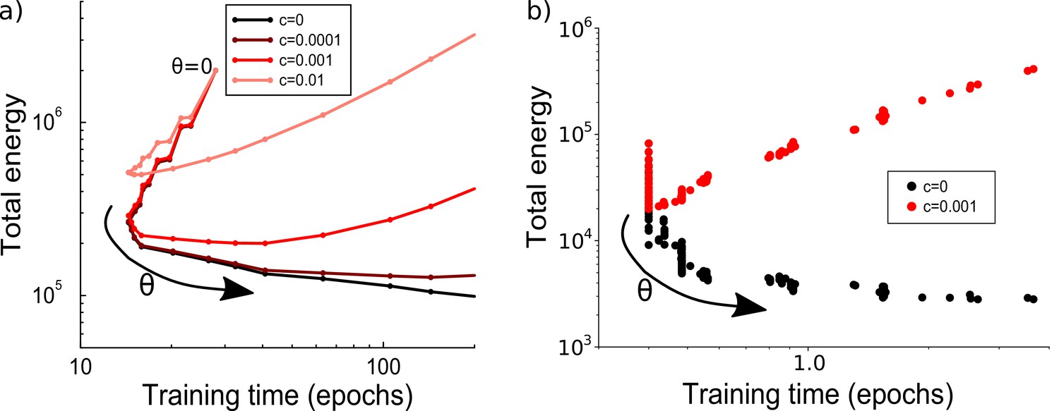
The effects of consolidation threshold on energy cost and learning time.
(a) Parametric plot of learning time vs energy while the consolidation threshold is varied. The threshold value runs from to 10 in steps of 0.5. For small maintenance costs, the threshold determines a trade-off between either a short learning time or a low energy (e.g. black curve). At higher maintenance costs, the most energy efficient threshold also leads to a short learning time. Average over 100 runs; parameter: . (b) Similar to the perceptron results in panel a, the effects of consolidation threshold on energy cost and learning time for training in a multi-layer network vary depending on the maintenance cost . Here, the threshold starts at 0.005 and is in increments of 0.005. When (black dots, each representing a unique consolidation threshold), there is a trade-off between shorter learning time and lower energy cost. When (red dots), the result is similar to the perceptron result with , where optimizing learning time or energy cost leads to a similar threshold. Parameters: , , required accuracy .
Figure 4
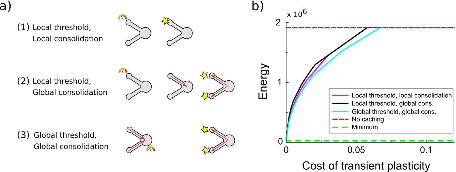
Comparison of various variants of the synaptic caching algorithm.
(a) Schematic representation of variants to decide when consolidation occurs. From top to bottom: (1) Consolidation (indicated by the star) occurs whenever transient plasticity at a synapse crosses the consolidation threshold and only that synapse is consolidated. (2) Consolidation of all synapses occurs once transient plasticity at any synapse crosses the threshold. (3) Consolidation of all synapses occurs once the total transient plasticity across synapses crosses the threshold. (b) Energy required to teach the perceptron is comparable across algorithm variants. Consolidation thresholds were optimized for each algorithm and each maintenance cost of transient plasticity individually. In this simulation the transient plasticity did not decay.
Figure 5
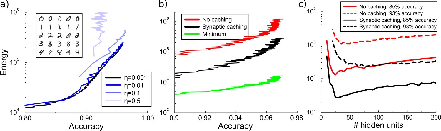
Energy cost to train a multilayer back-propagation network to classify digits from the MNIST data set.
(a) Energy rises with the accuracy of identifying the digits from a held-out test data. Except for the larger learning rates, the energy is independent of the learning rate . Inset shows some MNIST examples. (b) Comparison of energy required to train the network with/without synaptic caching, and the minimal energy. As for the perceptron and depending on the cost of transient plasticity, synaptic caching can reduce energy need manifold. (c) There is an optimal number of hidden units that minimizes metabolic cost. Both with and without synaptic caching, energy needs are high when the number of hidden units is barely sufficient or very large. Parameters for transient plasticity in (b) and (c): , , .
Figure 6
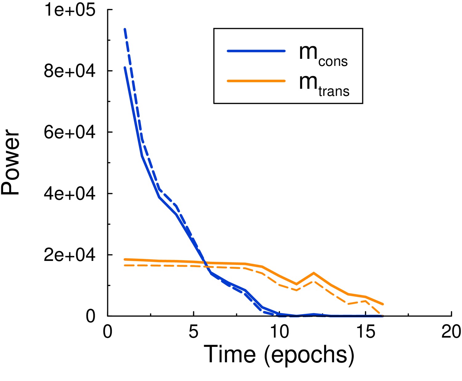
Maintenance and consolidation power.
Power (energy per epoch) of the perceptron vs epoch. Solid curves are from simulation, dashed curves are the theoretical predictions, Equations 6 and 7, with calculated by using the perceptron update rate extracted from the simulation. Both powers are well described by the theory. Parameters: , , .
Additional files
Download links
A two-part list of links to download the article, or parts of the article, in various formats.
Downloads (link to download the article as PDF)
Open citations (links to open the citations from this article in various online reference manager services)
Cite this article (links to download the citations from this article in formats compatible with various reference manager tools)
Energy efficient synaptic plasticity
eLife 9:e50804.
https://doi.org/10.7554/eLife.50804


