Research Article

Cell Biology

Magnetic resonance measurements of cellular and sub-cellular membrane structures in live and fixed neural tissue

Eunice Kennedy Shriver National Institute of Child Health and Human Development, National Institutes of Health, United States
Celoptics, United States
Center for Neuroscience and Regenerative Medicine, Henry Jackson Foundation, United States
National Institute of Neurological Disorders and Stroke, National Institutes of Health, United States
National Institute of Mental Health, National Institutes of Health, United States
National Heart, Lung, and Blood Institute, National Institutes of Health, United States
Zhejiang University, China

Dec 12, 2019

https://doi.org/10.7554/eLife.51101

Open access
Copyright information

Figures
Tables
Additional files

17 figures, 1 table and 1 additional file

Figures

Figure 1 with 1 supplement

Download asset Open asset

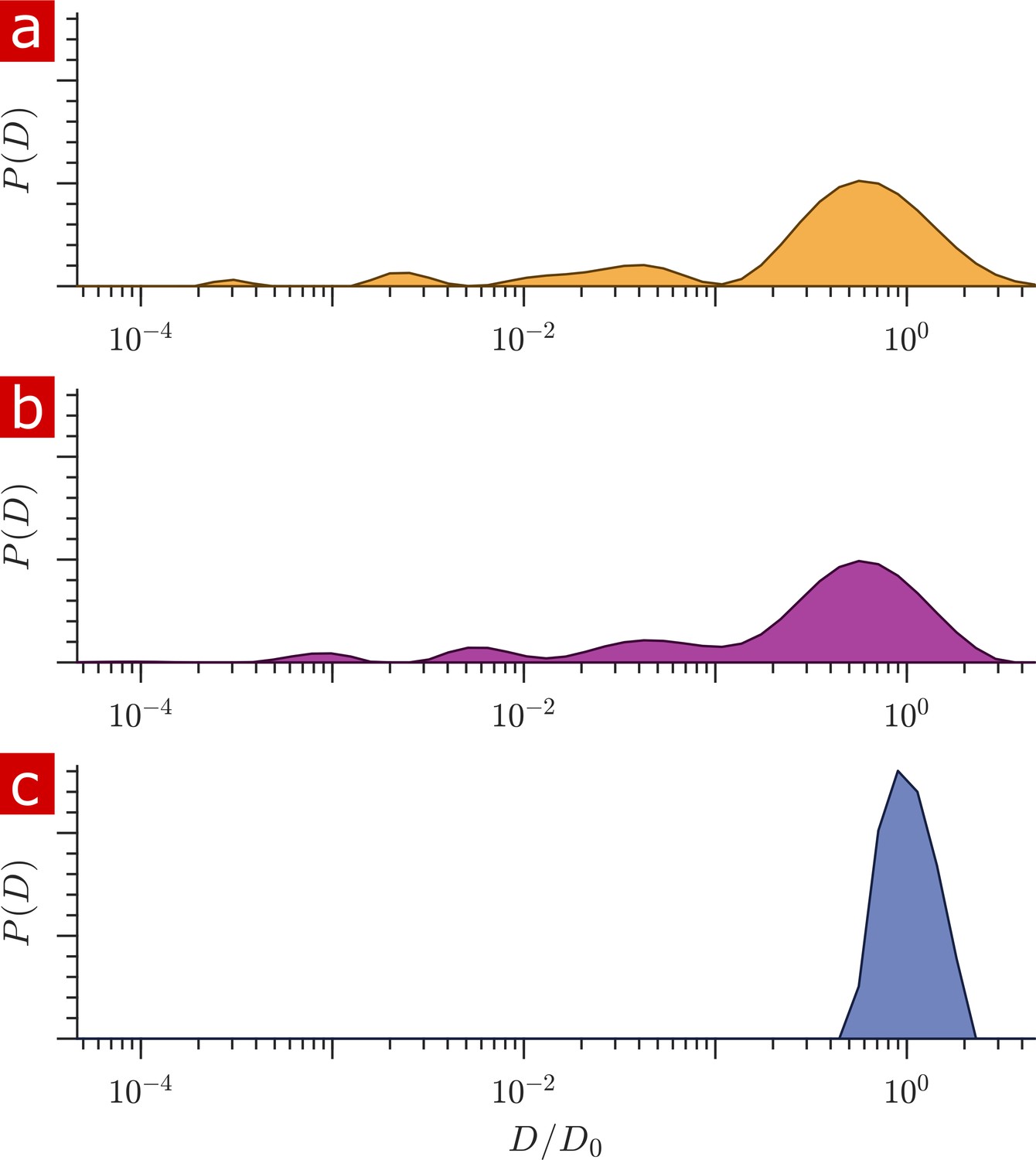
Diffusion coefficient distributions.

(a) Distribution of diffusion coefficients from a fixed spinal cord bathed in aCSF. (b) Distribution from the same spinal cord after removing the aCSF bath. (c) Distribution from only aCSF filling the RF coil.

Figure 1—source data 1 1-D Diffusion signal attenuation ( $I$ ) and $b$ values for the measurements on fixed spinal cord bathed in aCSF (wet), the same spinal cord after removing aCSF (dry), and for aCSF (MATLAB structure array). 1-D Diffusion signal attenuation ( $I$ ) and $b$ values for repeated measurements on aCSF (MATLAB structure array).: https://cdn.elifesciences.org/articles/51101/elife-51101-fig1-data1-v2.mat
Download elife-51101-fig1-data1-v2.mat
Figure 1—source data 2 1-D Diffusion signal attenuation ( $I$ ) and $b$ values for repeated measurements on aCSF (MATLAB structure array).: https://cdn.elifesciences.org/articles/51101/elife-51101-fig1-data2-v2.mat
Download elife-51101-fig1-data2-v2.mat

Figure 1—figure supplement 1

Download asset Open asset

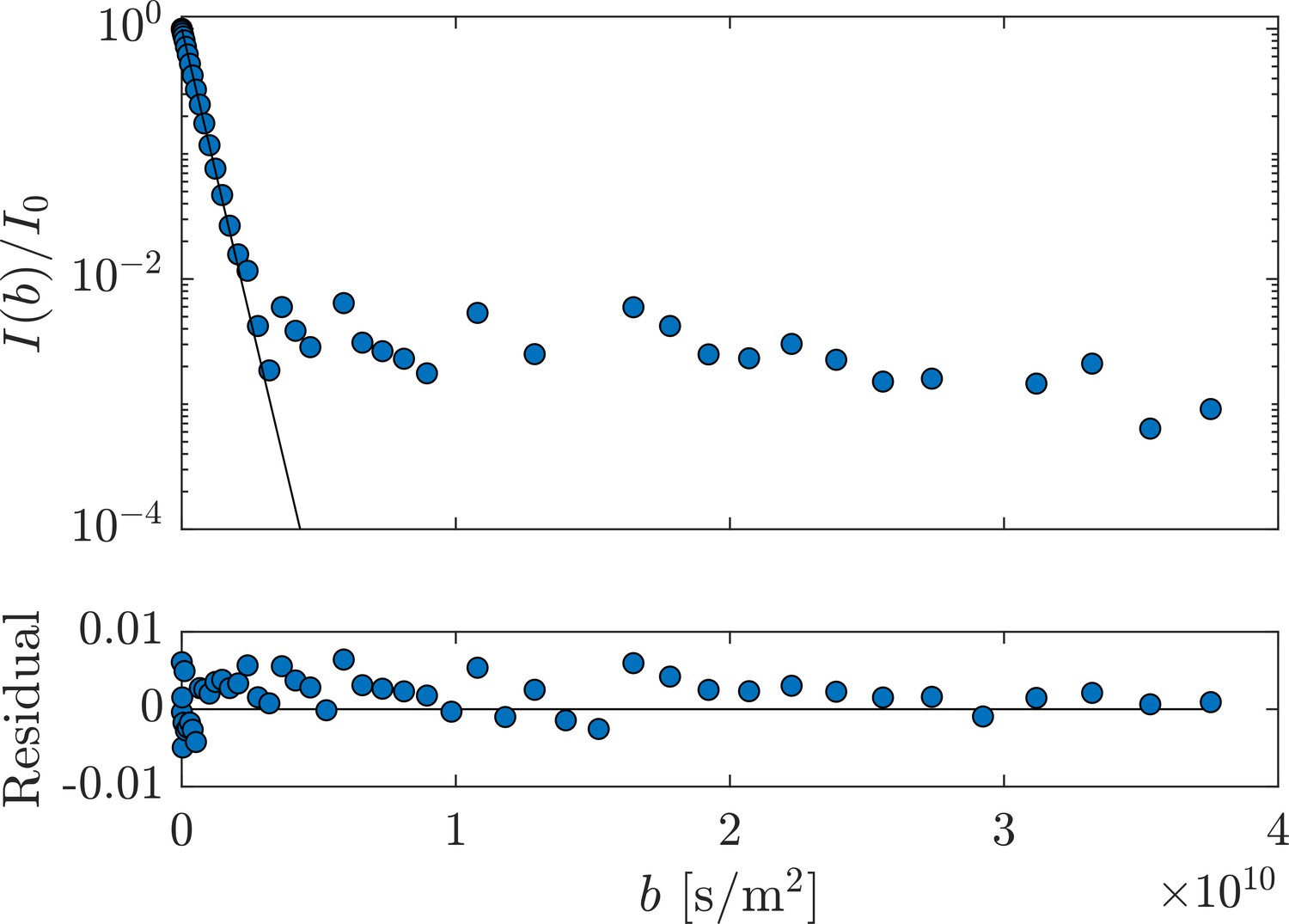
Measurement of aCSF $D_{0}$ at 25°C.

Single exponential fits of the first 15 of the 50 points, attenuating the signal to $I / I_{0} = 0.1$ , provides D₀ = 2.153 ± 0.014 × 10⁻⁹ m²/s from three measurements performed on only aCSF filling the coil. Fit residuals are also shown.

Figure 2 with 1 supplement

Download asset Open asset

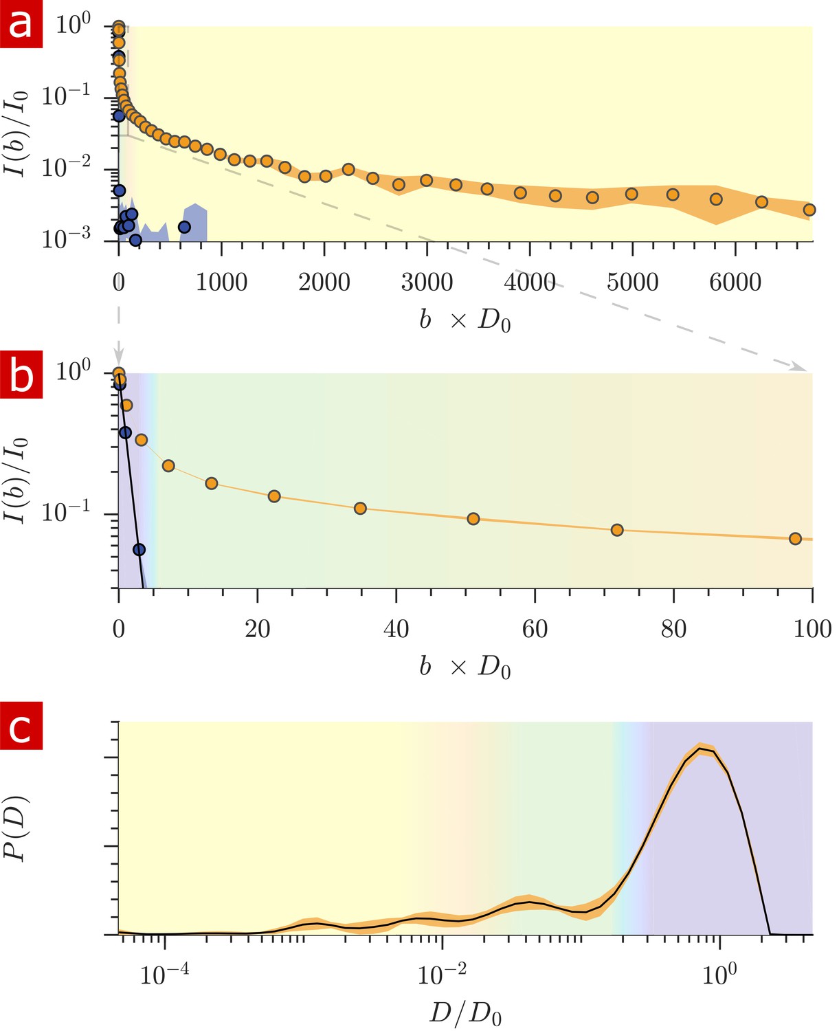
Diffusion measurements performed on a fixed spinal cord.

(a) Mean (circles) and SD (shaded bands) of the signal intensity from five diffusion measurements, spaced 54 min apart, performed on a fixed spinal cord (orange) and three measurements performed on aCSF (purple) at 25° C. (b) Signal intensity from the zoomed in area shown in (a). (c) The distribution of diffusion coefficients resulting from inversion of the data. The purple, green, and yellow shading across plots signifies water which is free, less restricted, and more restricted, respectively. Models of signal attenuation (see Appendix 1) are used to define the cutoffs for each of these regimes based on when their signal components would attenuate to exp (−6). Values are inverted to define the color shading on the $D$ distribution. This inversion of colors is simply to guide the eye. The color gradient is meant to signify a continuous change between diffusion regimes rather than sharp boundaries.

Figure 2—source data 1 1-D Diffusion signal attenuation ( $I$ ) and $b$ values for measurements repeated every 54 min on a fixed spinal cord (MATLAB structure array).: https://cdn.elifesciences.org/articles/51101/elife-51101-fig2-data1-v2.mat
Download elife-51101-fig2-data1-v2.mat

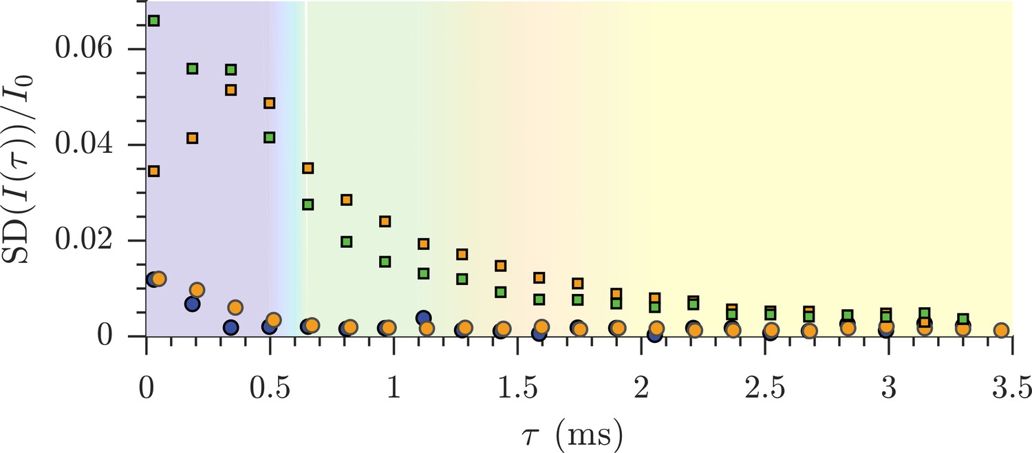
Figure 2—figure supplement 1

Download asset Open asset

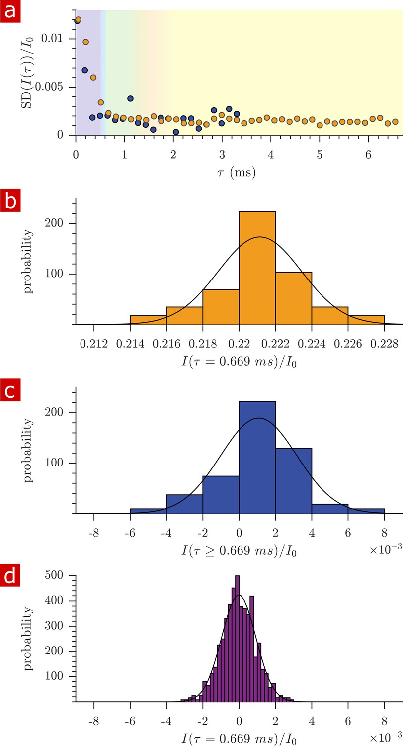
Variability of diffusion data from measurements repeated on the same samples.

(a) Standard deviation (SD) of the signal intensity from 29 diffusion measurements, spaced 54 min apart, performed on a fixed spinal cord (orange) and three measurements performed back-to-back on aCSF (purple) at 25° C. Data is from the same samples as in Figure 2. (b) Histogram of signal intensity from measurements on the fixed spinal cord at $τ = 0.669$ ms with mean ± SD 0.2211 ± 0.0023. (c) Histogram from the measurements on aCSF at $τ \geq 0.669$ ms, after signal has decayed away, with mean ± SD 0.0011 ± 0.0021. (d) Histogram of noise from 621 diffusion measurements performed on a dry chamber with nothing filling the solenoid coil, with mean ± SD = −2× 10⁻⁵ ± 0.001. In (b), (c) and (d), Gaussian distributions are plotted using the mean and SD as parameters μ and $σ$ . Note the similar window width in (b), (c), and (d) allow comparison of SD. (See also Appendix 2).

Figure 3 with 1 supplement

Download asset Open asset

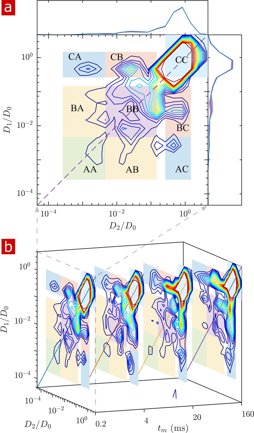
Full 2-D DEXSY diffusion exchange distribution for a fixed spinal cord.

(a) Exchange distribution measured with mixing time $t_{m} = 0.2 ms$ . Distributions show exchanging (off-diagonal) and non-exchanging (on-diagonal) components. These components are lumped into regions $A$ , $B$ , and $C$ , shaded and labeled in a 3 × 3 grid for each exchange combination. The range of $P (D_{1}, D_{2})$ is set to add detail to components $A$ and $B$ , but cuts off the top of the most mobile region $CC$ . The marginal distributions $P (D_{1})$ and $P (D_{2})$ are presented on the sides, with mean (solid blue lines) and SD (shaded bands around lines) from three measurements. (b) A stacked view of distributions measured with mixing time $t_{m} = [0.2, 4, 20, 160] ms$ . With increasing $t_{m}$ , the probability density builds up in regions of free and restricted water exchange $AC + CA$ and $BC + CB$ and decays for non-exchanging restricted water regions $AA$ and $BB$ .

Figure 3—source data 1 Full 2-D DEXSY datasets from measurements repeated three times at each mixing time on each of the fixed samples (MATLAB structure array).: https://cdn.elifesciences.org/articles/51101/elife-51101-fig3-data1-v2.mat
Download elife-51101-fig3-data1-v2.mat

Figure 3—figure supplement 1

Download asset Open asset

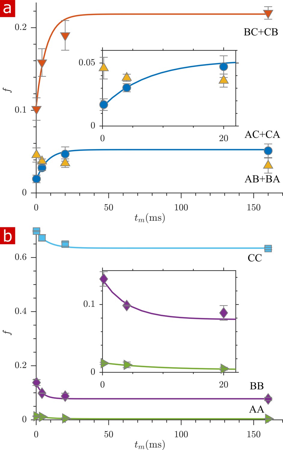
Fractions of exchanging and non-exchanging water.

(a) Fractions of water which exchange between regions $A$ , $B$ , and $C$ , (defined in Figure 3a) as a function of mixing time, $t_{m}$ . Exchange fractions $f_{AC + CA}$ and $f_{BC + CB}$ are fit with a first-order rate model with estimated apparent exchange rates AXRs (mean ± standard deviation from three measurements) 140 ± 80 and 140 ±140 s⁻¹, respectively. $f_{AB + BA}$ does not follow the expected first-order rate model. (b) Fractions of non-exchanging water. Non-exchange fractions $f_{AA}$ , $f_{BB}$ , and $f_{CC}$ are fit with a first-order rate model with estimated AXRs 110 ± 100, 230 ± 170, and 130 ±100 s⁻¹ respectively. Insets zoom in on the initial rise in exchange. Error bars are the standard deviations from three repeat measurements.

Figure 4 with 1 supplement

Download asset Open asset

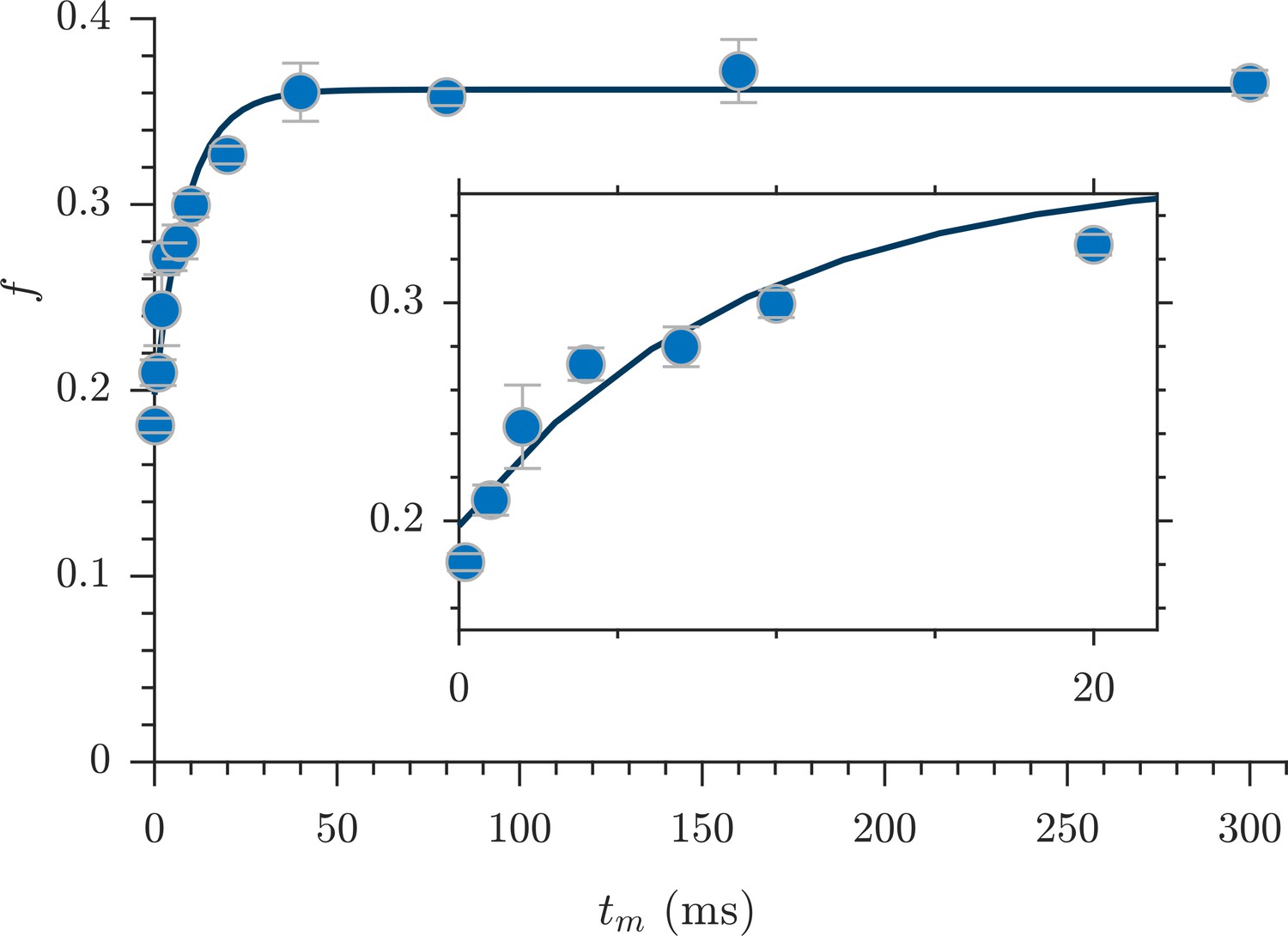
Rapid measurement of exchange fractions.

A fit of the first-order rate model estimated an apparent exchange rate, AXR = 110 ± 30 s⁻¹ (mean ± SD from three measurements performed on one specimen at 25°C). Inset shows a zoomed-in region of the initial rise in exchange.

Figure 4—source data 1 Rapid exchange data for all fixed samples, including raw data from the four-point method ( $I$ ) and the exchange fractions ( $f$ ) (MATLAB structure array).: https://cdn.elifesciences.org/articles/51101/elife-51101-fig4-data1-v2.mat
Download elife-51101-fig4-data1-v2.mat

Figure 4—figure supplement 1

Download asset Open asset

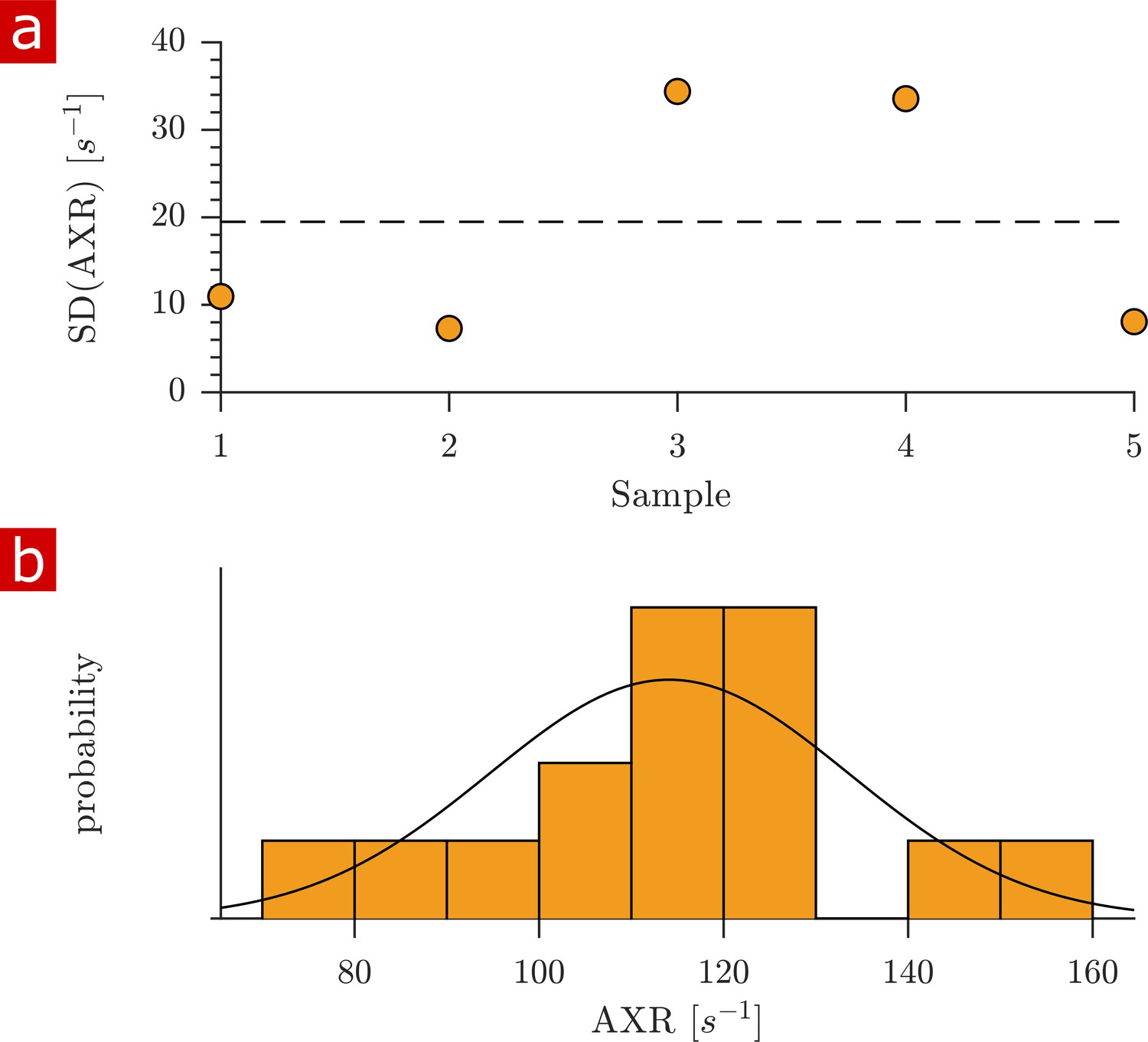
Variability of apparent exchange rates (AXRs).

(a) Standard deviations of AXRs from three rapid exchange measurements shown for five fixed spinal cord samples. The dashed line shows the SD from all (3 × 5) measurements. (b) Histogram of all measured AXRs with mean = 114 and SD = 19 s⁻¹. A Gaussian distribution is plotted using the mean and SD as parameters μ and $σ$ . An Anderson–Darling test indicates that the distribution is not dissimilar from a Gaussian distribution ( $P = 0.88 > 0.05$ ).

Figure 5

Download asset Open asset

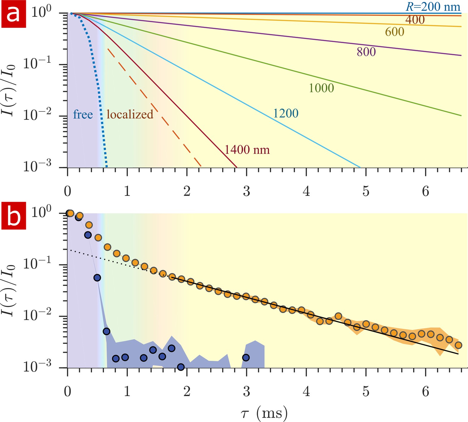
Sensitivity to membrane structure sizes from the diffusion signal attenuation.

(a) Signal intensity is simulated for water restricted in spherical compartments of varying radius between R = 200 − 1400 nm (solid lines) (Neuman, 1974), for water localized near surfaces in larger restrictions (red dashed line) (de Swiet and Sen, 1994; Hurlimann et al., 1995), as well as water diffusing freely (purple dotted line) (Woessner, 1961). Signal is plotted as a function of the variable $τ$ (rather than $b \sim τ^{3}$ ). (b) Signal is re-plotted from Figure 2. Signal at $τ \geq 1.8$ ms is fit with the model for water restricted in spherical compartments in the limit of long $τ$ (solid black line) (Neuman, 1974) incorporating the AXR = 110 s⁻¹(Carlton et al., 2000), estimating a radius R = 900 nm. The dotted black line extrapolates back to $I / I_{0} = 0.2$ . (See Appendix 1 for model equations.) Color shading is similar to Figure 2.

Figure 6 with 1 supplement

Download asset Open asset

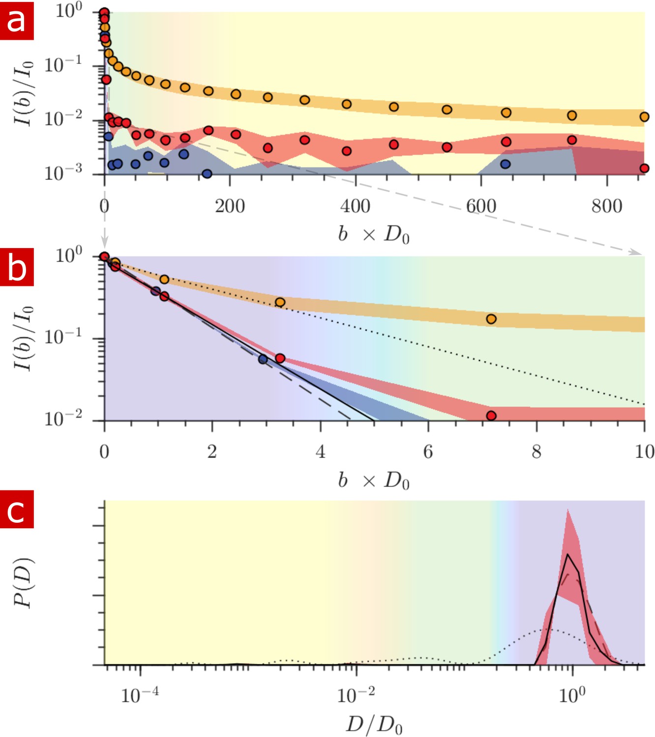
Diffusion in fixed vs. live.

(a) Signal intensity from diffusion measurements performed at 25° C on live samples (n = 9) (green squares), fixed samples (n = 6) (orange circles) and aCSF (purple circles) plotted as a function of the variable $τ$ . (b) Mono- and poly- synaptic reflexes were recorded from the L6 ventral root of live samples (n = 4) after NMR measurements. Stimulation was done on the homonymous dorsal root. The grey lines are five successive stimuli (30 s interval) and the superimposed red line is the average signal. The arrow indicates the stimulus artifact and the star the monosynaptic reflex.

Figure 6—source data 1 1-D diffusion data for all fixed and live samples (MATLAB structure array).: https://cdn.elifesciences.org/articles/51101/elife-51101-fig6-data1-v2.mat
Download elife-51101-fig6-data1-v2.mat

Figure 6—figure supplement 1

Download asset Open asset

Sample-to-sample variability of diffusion data.

Standard deviations of the diffusion signal attenuation are presented for live (n = 9) (green squares) and fixed (n = 6) (orange circles) sample groups. The standard deviations from repeated measurements are also re-plotted from Figure 2—figure supplement 1a. The sample-to-sample variability is higher that the variability of repeated measurements due to structural and size differences between samples and the sensitivity of the measurement to these differences.

Figure 7 with 3 supplements

Download asset Open asset

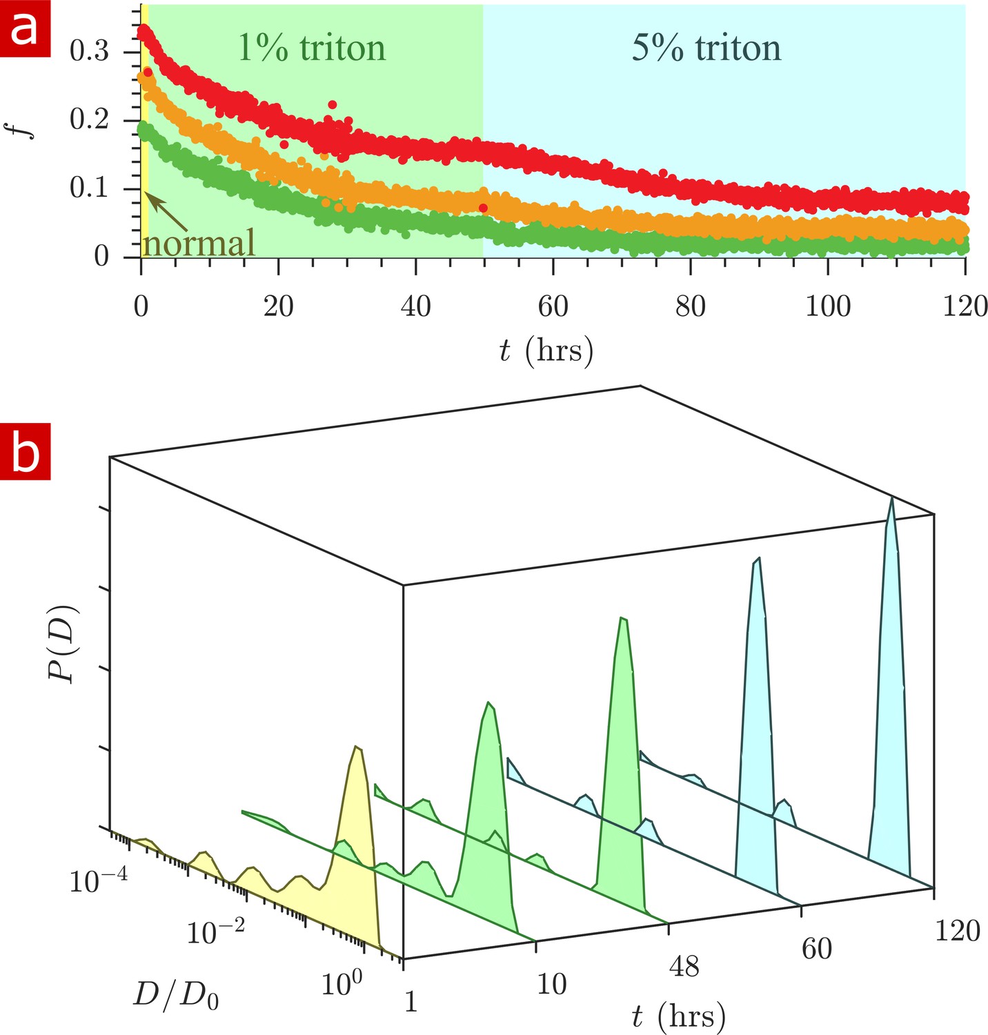
Timecourse study of Triton X delipidation.

(a) Exchange fractions from rapid exchange measurements with $t_{m} = 0.2$ (green dots), 4 (orange dots), and 20 ms (red dots) measured throughout the timecourse, as the sample was washed to aCSF with 1% Triton X, and then 5% Triton X. (b) Representative diffusion coefficient distributions from 1-D diffusion measurements performed at different times before and after addition of Triton.

Figure 7—source data 1 1-D diffusion data for real-time delipidation of a fixed spinal cord (MATLAB structure array).: https://cdn.elifesciences.org/articles/51101/elife-51101-fig7-data1-v2.mat
Download elife-51101-fig7-data1-v2.mat

Figure 7—figure supplement 1

Download asset Open asset

Timecourse of restriction during Triton X delipidation.

The fraction (a) and mean diffusion coefficient (b) of signal arising from restricted water (with $D / D_{0} < 0.17$ ). A bump in the restricted fraction seen upon addition of the 5% Triton is due to the Triton X itself which forms 5 nm micelles (Paradies, 1980).

Figure 7—figure supplement 2

Download asset Open asset

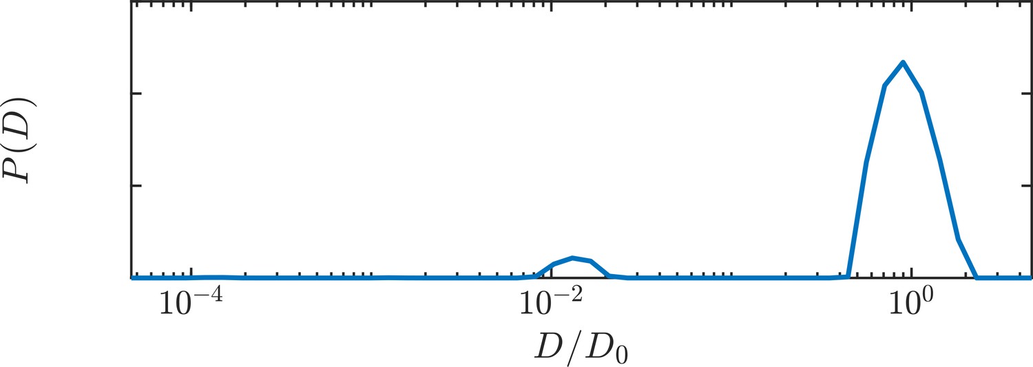
Diffusion coefficient distributions of 5% Triton X in aCSF.

An additional peak at $D / D_{0} = 0.013$ is due to formation of 5 nm micelles (Paradies, 1980).

Figure 7—video 1

Download asset

posterframe for video — Timelapse video of diffusion coefficient distributions during delipidation.

Each frame is spaced 54 min apart and the whole video represents 120 hr of delipidation. See Figure 7 for times as which the sample was washed to aCSF with 1% Triton X and 5% Triton X. The final distribution at 120 hr looks very similar to the distribution for 5% TritonX in aCSF.

Figure 8

Download asset Open asset

Diffusion measurement after delipidation.

(a) Diffusion signal intensity from measurements on spinal cords performed at 25° C after delipidation (n = 2) with 10% Triton X and after washing the Triton away. The mean (circles) and SD (shaded bands) of the attenuation are plotted for the delipidated samples (red) alongside pure aCSF (purple) and fixed undelipidated spinal cords (n = 6) (orange). (b) The initial attenuation of signal. Monoexponential fits of the attenuation from points 2–4 yielded 2.15 ± 0.02, 1.94 ± 0.02 and 0.87 ± 0.14 ×10⁻⁹ m²/s for the aCSF, delipidated, and undelipidated spinal cords and are shown as the dashed, solid, and dotted lines, respectively. (c) Diffusion coefficient distribution of the delipidated spinal cords, for which the mean (solid line) and SD (shaded band around line) are not significantly different from the pure aCSF (dashed line). The distribution from a fixed, undelipidated spinal cord (dotted line) is also shown for comparison. The purple, green, and yellow shading across the plots signifies water which is free, localized, and restricted.

Figure 9

Download asset Open asset

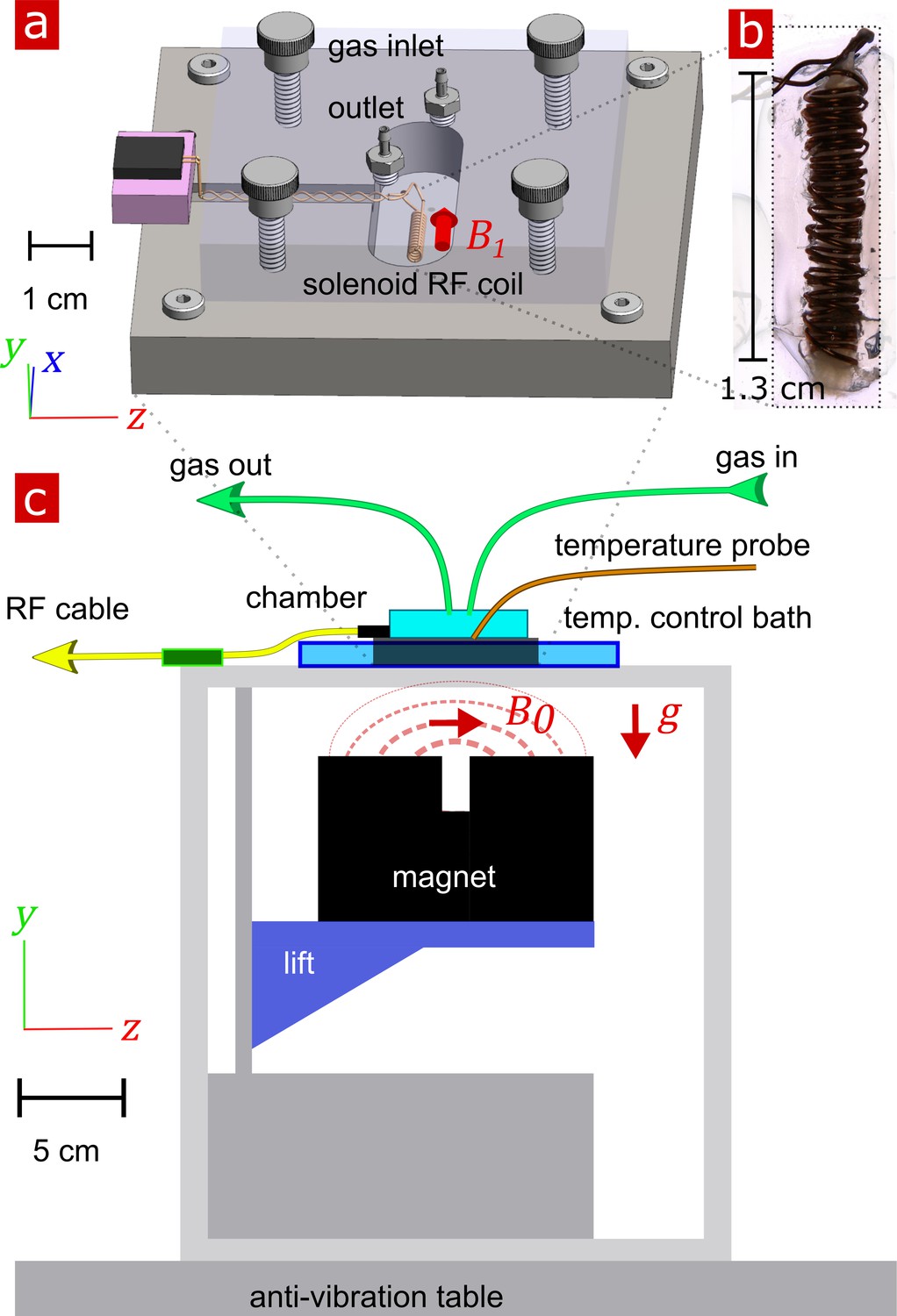
Experimental setup.

(a) 3-D technical drawing of the test chamber. (b) Image of the solenoid RF coil containing a fixed, delipidated specimen. (c) Technical drawing of the experimental setup. The magnet is drawn in the ‘service’ position to show the field lines extending from one magnetic pole to the other. To perform measurements, the magnet would be raised such that the $B_{0}$ was correctly positioned relative to the sample. Vectors $B_{1}$ , $g$ and $B_{0}$ point in the $x$ , $y$ , and $z$ directions respectively.

Appendix 3—figure 1

Download asset Open asset

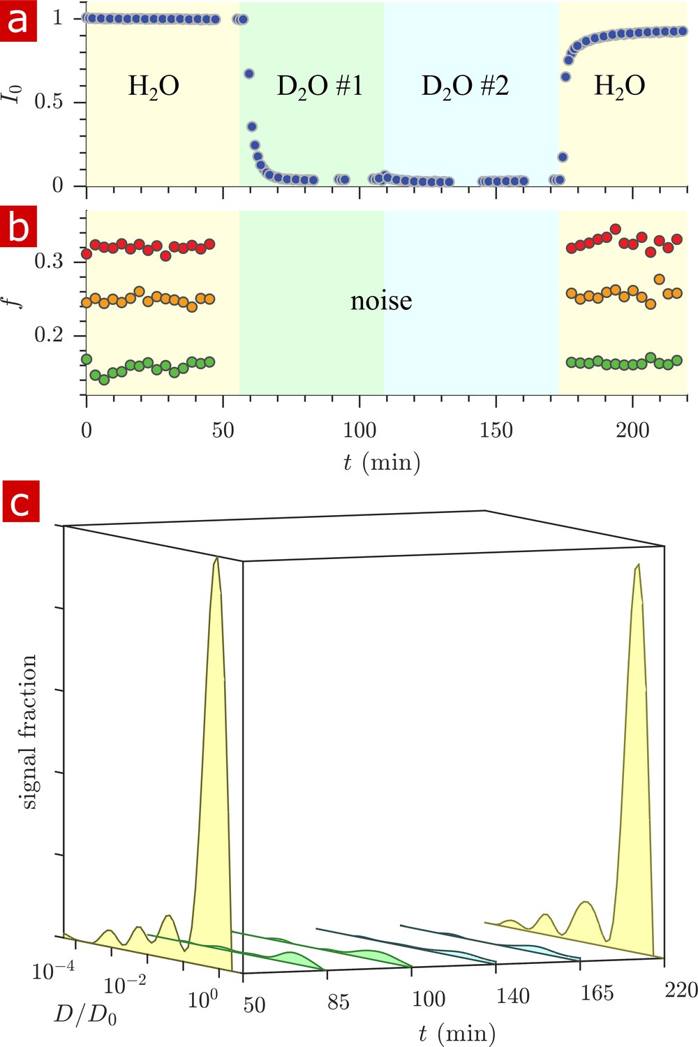
Timecourse study of D₂O wash.

The sample was washed from aCSF to aCSF made with deuterated water in two steps and back to aCSF as shown by the yellow, green, blue, and yellow pastel color shadings for H₂O, D₂O #1, D₂O #2, and H₂O. (a) The proton signal intensity from rapid exchange measurement data normalized to remove $T_{1}$ effects at different mixing times. (b) Exchanging fractions from rapid measurements with $t_{m} = 0.2$ (blue), 4 (red), and 20 ms (orange). (c) 1-D diffusion measurements were performed at points throughout the timecourse (seen as breaks in the data in (a)) and distributions are presented as signal fractions ( $P (D) \times I_{0}$ ).

Appendix 5—figure 1

Download asset Open asset

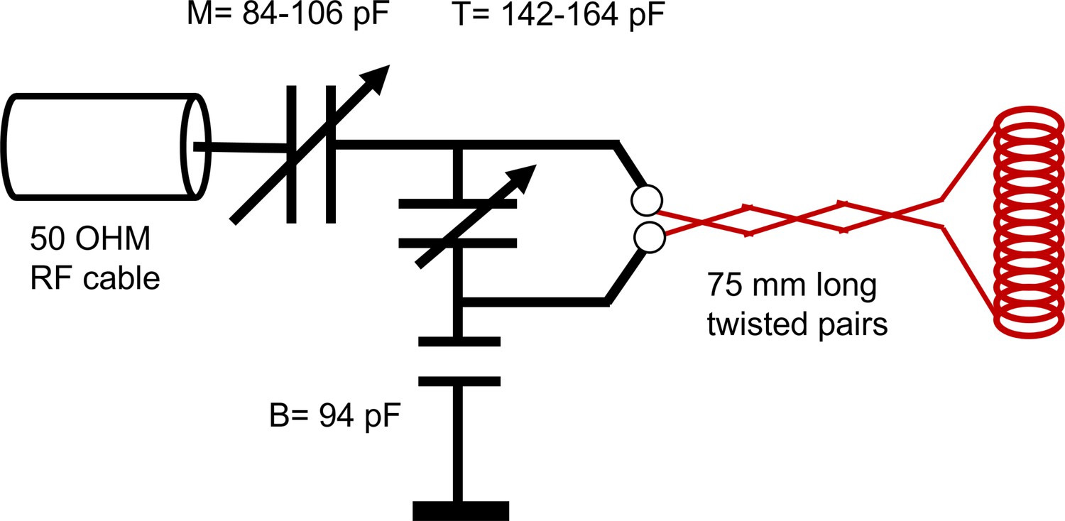
RF circuit design.

Drawing of the circuit for the RF showing the capacitance of the tune (T), match (M), and balance (B). Note a single wrapping of the solenoid was drawn rather than the actual double-wrap for visual simplicity.

Appendix 5—figure 2

Download asset Open asset

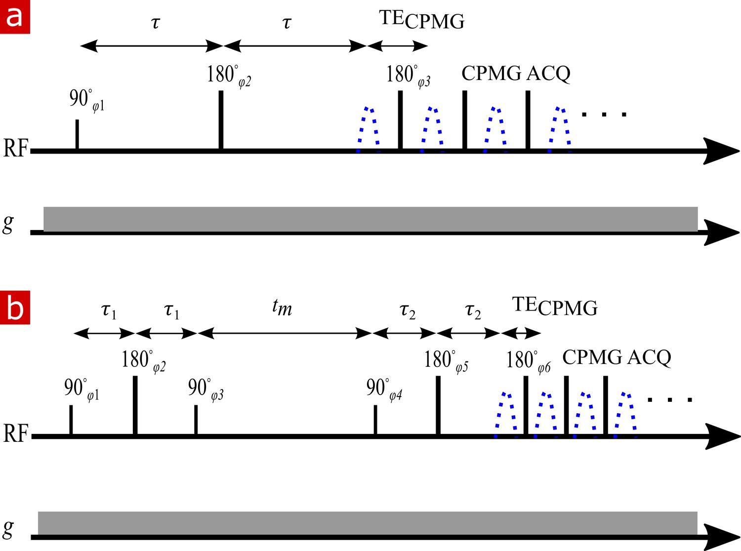
NMR diffusion and exchange pulse sequences.

(a) Spin echo pulse sequence for measuring diffusion with a static gradient. $τ$ is varied to control $b$ . (b) DEXSY pulse sequence for measuring exchange with a static gradient. The two SE encoding blocks with $τ_{1}$ and $τ_{2}$ , varied independently to control $b_{1}$ and $b_{2}$ , are separated by $t_{m}$ . Signal is acquired in a CPMG train for both (a) and (b).

Appendix 6—figure 1

Download asset Open asset

$T_{2}$ measurement.

Representative Carr-Purcell-Meiboom-Gill (CPMG) (10 s repetition time (TR), 8000 echoes, TE = 25 μs) on fixed spinal cord. (a) The echo shape summed over all echoes (real signal (blue) phased maximum and imaginary signal phased to zero (red)). (b) Real signal decay (orange circles) and exponential fit with $T_{2} = 163$ ms and $I_{0} = 6.5 μ V$ (white line) and residuals of the fit.

Appendix 6—figure 2

Download asset Open asset

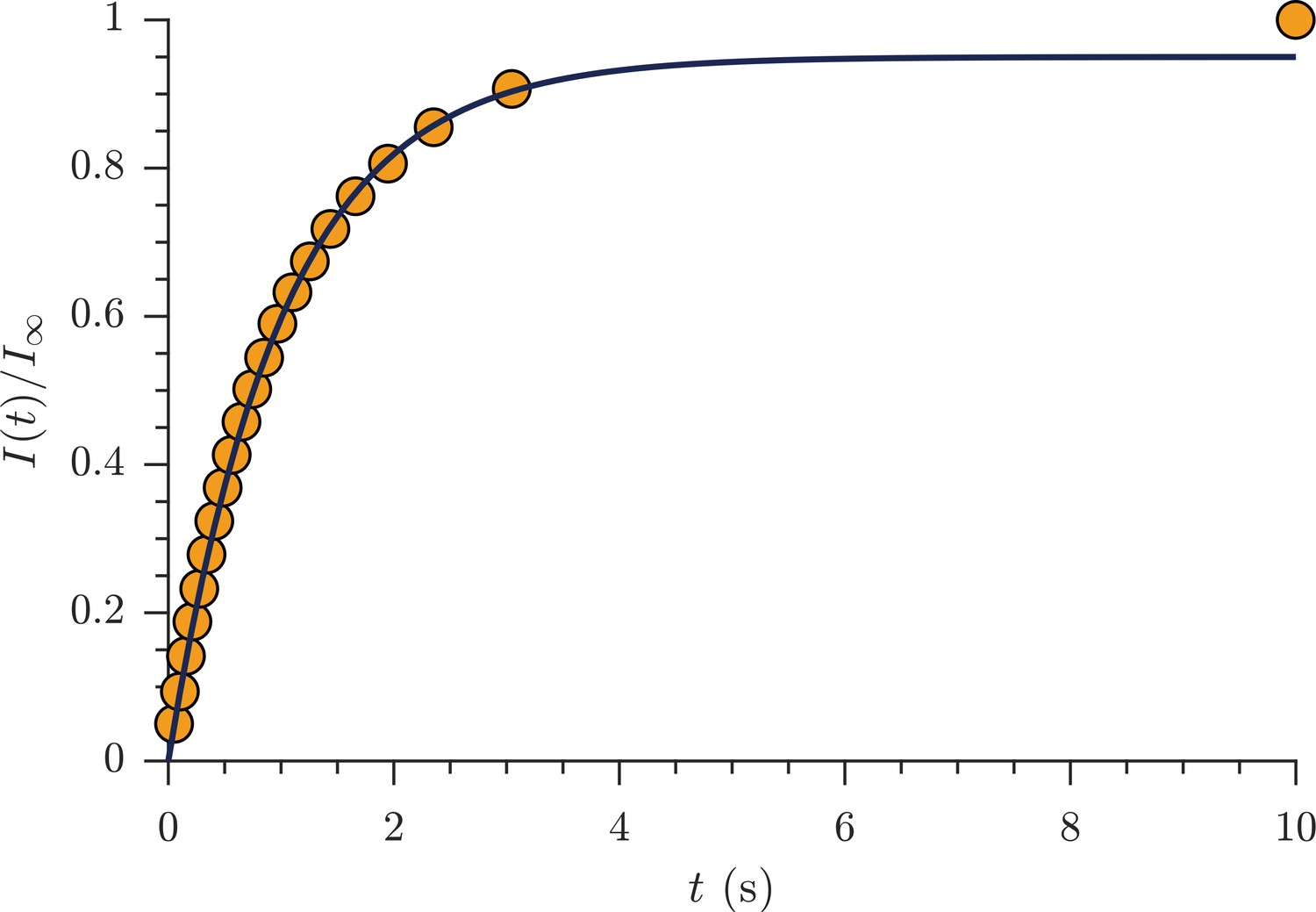
$T_{1}$ measurement.

Representative saturation recovery experiment on fixed spinal cord (1 s TR, 21 recovery time points logarithmically spaced from 50 ms to 10 s) showing signal intensity normalized by signal at 10 s recovery time (orange circles) and exponential fit with estimated T₁ = 990 ms (solid black line).

Appendix 7—figure 1

Download asset Open asset

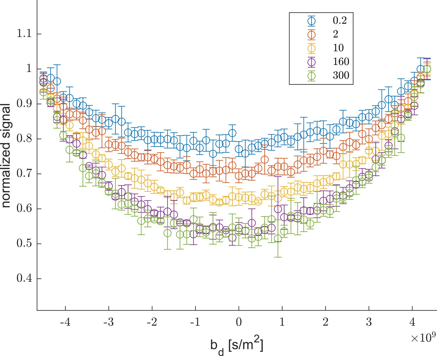
Rapid exchange test #1.

The curvature along slices of $b_{s} = 4500 s / {mm}^{2}$ as a function of $b_{d}$ highlighting the increase in the depth of the curvature with increasing $t_{m}$ , shown in figure legend. The increased depth is due to increased exchange (Song et al., 2016; Cai et al., 2018).

Appendix 7—figure 2

Download asset Open asset

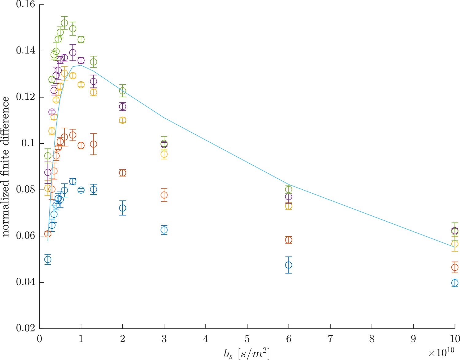
Rapid exchange test #2.

Difference between $2 I_{b_{d} = 0}$ and $I_{b d = + b s} + I_{b d = - b s}$ , normalized by $I_{0, 0}$ , as a function of $b_{s}$ , showing the optimal $b_{s}$ for measuring the largest curvature response as occurring near $b_{s} = 6000 s / {mm}^{2}$ . The line is a prediction of the finite difference for a two-site system, from Equation 8 in Cai et al. (2018) using $f = 0.15$ , $D_{e} = 10^{- 9}$ , and $D_{i} = 10^{- 11} s / {mm}^{2}$ .

Appendix 7—figure 3

Download asset Open asset

Rapid exchange test #3.

High temporal resolution exchange rate measurement from the rapid measurement with $b_{s} = 4500 s / {mm}^{2}$ and 53 $t_{m}$ points between 0.1 and 300 ms. First order rate model fits estimate AXR = 113.7 ± 5.2 s⁻¹ (solid line).

Tables

Appendix 5—table 1

Static gradient spin echo DEXSY Phase Cycles.

φ₁	φ₂	φ₃	φ₄	φ₅	φ₆	φ_rec
0	+π/2	0	0	+π/2	π/2	π
π	-π/2	0	0	+π/2	π/2	0
0	+π/2	π	0	+π/2	π/2	0
π	-π/2	π	0	+π/2	π/2	π
0	+π/2	0	π	-π/2	π/2	0
π	-π/2	0	π	-π/2	π/2	π
0	+π/2	π	π	-π/2	π/2	π
π	-π/2	π	π	-π/2	π/2	0

Additional files

Transparent reporting form: https://cdn.elifesciences.org/articles/51101/elife-51101-transrepform-v2.docx
Download elife-51101-transrepform-v2.docx

Download links

A two-part list of links to download the article, or parts of the article, in various formats.

Downloads (link to download the article as PDF)

Open citations (links to open the citations from this article in various online reference manager services)

Mendeley

Cite this article (links to download the citations from this article in formats compatible with various reference manager tools)

Nathan H Williamson
Rea Ravin
Dan Benjamini
Hellmut Merkle
Melanie Falgairolle
Michael James O'Donovan
Dvir Blivis
Dave Ide
Teddy X Cai
Nima S Ghorashi
Ruiliang Bai
Peter J Basser

(2019)

Magnetic resonance measurements of cellular and sub-cellular membrane structures in live and fixed neural tissue

eLife 8:e51101.

https://doi.org/10.7554/eLife.51101

Share this article

Cite this article

Diffusion coefficient distributions.

Figure 1—source data 1

Figure 1—source data 2

Measurement of aCSF D0 at 25°C.

Diffusion measurements performed on a fixed spinal cord.

Figure 2—source data 1

Variability of diffusion data from measurements repeated on the same samples.

Full 2-D DEXSY diffusion exchange distribution for a fixed spinal cord.

Figure 3—source data 1

Fractions of exchanging and non-exchanging water.

Rapid measurement of exchange fractions.

Figure 4—source data 1

Variability of apparent exchange rates (AXRs).

Sensitivity to membrane structure sizes from the diffusion signal attenuation.

Diffusion in fixed vs. live.

Figure 6—source data 1

Sample-to-sample variability of diffusion data.

Timecourse study of Triton X delipidation.

Figure 7—source data 1

Timecourse of restriction during Triton X delipidation.

Diffusion coefficient distributions of 5% Triton X in aCSF.

Timelapse video of diffusion coefficient distributions during delipidation.

Diffusion measurement after delipidation.

Experimental setup.

Timecourse study of D2O wash.

RF circuit design.

NMR diffusion and exchange pulse sequences.

T2 measurement.

T1 measurement.

Rapid exchange test #1.

Rapid exchange test #2.

Rapid exchange test #3.

Static gradient spin echo DEXSY Phase Cycles.

Transparent reporting form

Downloads (link to download the article as PDF)

Open citations (links to open the citations from this article in various online reference manager services)

Cite this article (links to download the citations from this article in formats compatible with various reference manager tools)

Measurement of aCSF $D_{0}$ at 25°C.

Timecourse study of D₂O wash.

$T_{2}$ measurement.

$T_{1}$ measurement.