Hippocampal remapping as hidden state inference
- Center for Brains Minds and Machines, Harvard University, United States
- Picower Institute for Learning and Memory and Department of Brain and Cognitive Sciences, Massachusetts Institute of Technology, United States
- Department of Psychology, Harvard University, United States
Figures
Figure 1
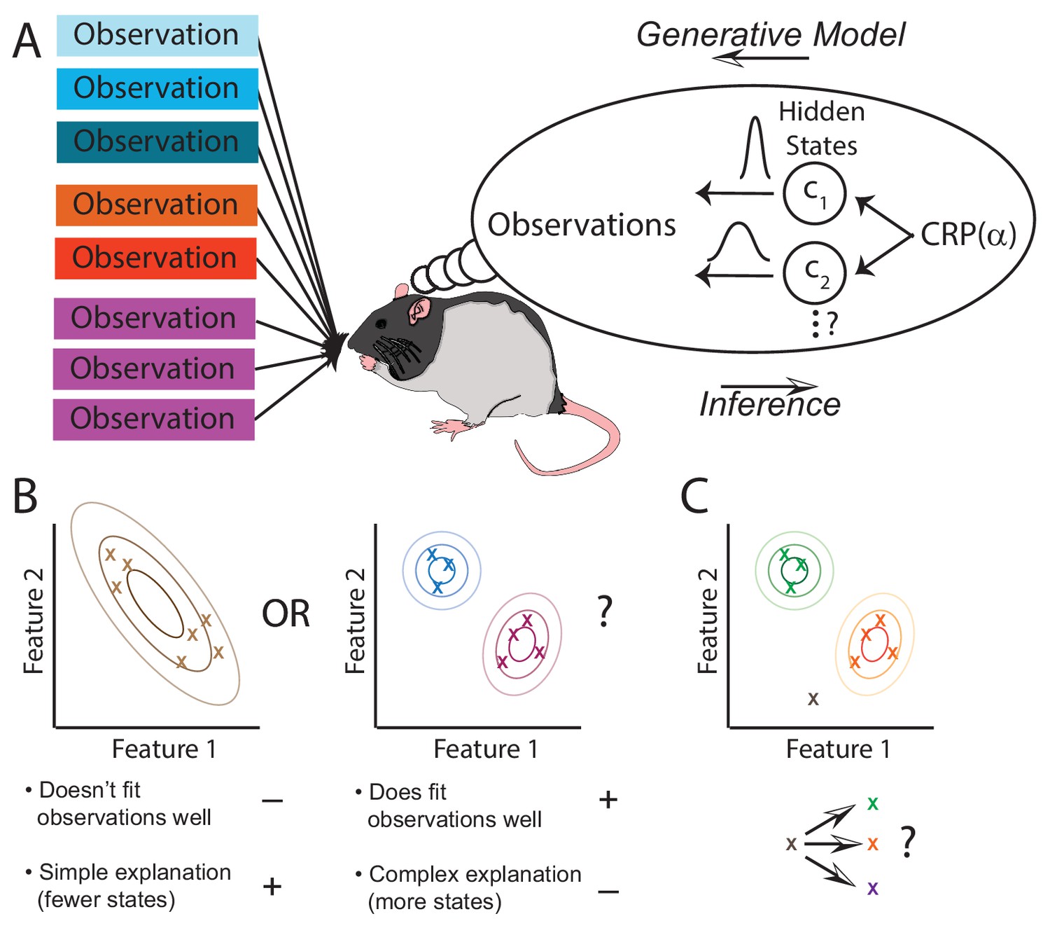
The hidden state inference framework.
(A) Schematic of hidden state inference. We impute an internal generative model to the animal, according to which observations are generated by a small number of hidden states. States are sampled from the Chinese Restaurant Process, parametrized by (see Materials and methods for details). Each state is associated with a particular distribution over observations. The animal receives those observations but does not have direct access to the states that generated them. We model the animal as probabilistically inverting this generative model by computing the posterior distribution over hidden states given observations. (B) Example inference problem. Given a set of observations (x’s), the animal must infer how many hidden states there are. There is a tradeoff between increasing the number of hidden states in order to better fit the observations vs. decreasing the number of states in order to decrease the complexity of the explanation. The partition evidence ratio can be calculated given a particular set of observations to express the relative preference for the 1-state model vs. the 2-state model. See Equation 7 in the Materials and methods section for more details. (C) Another example inference problem. Given an assignment of past observations (green and orange x’s) to hidden states (green and orange) and a novel observation (gray x), the animal forms a belief about hidden state assignment of the novel observation. This belief consists of probabilities of assigning the novel observation to each of the past hidden states (green or orange) or alternatively to a novel hidden state (purple). We can compare any two of these alternatives with the state evidence ratio. See Equation 11 in the Materials and methods section for more details.
Figure 2
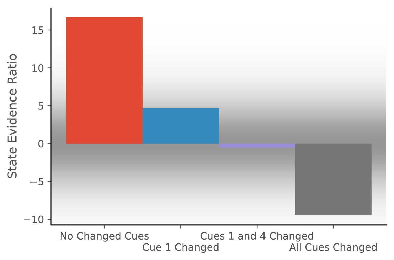
Hidden state inference is informed by cue constellations.
Observations are generated from a distribution with four features, each drawn from a Gaussian with mean 0 and standard deviation of 0.2.We train the model with 20 observations drawn from that distribution. We then compare the posterior probability of assigning a probe observation to the same hidden state as the previous observations vs. assigning it to a novel hidden state (Equation 11 for same vs. novel ). The first probe is an observation where each feature has a value of 0 (no cues changed). The model prefers assigning this probe observation to the same hidden state as the previous observations, corresponding to no remapping. The second probe is an observation where the first feature has a value of 1 and the other features have values of 0 (cue one changed). The third probe is an observation where the first and last features have a value of 1 and the other features have values of 0 (cues 1 and 4 changed). For both of these, the model assigns a state evidence ratio near 0, representing relatively high uncertainty about hidden state assignment, which corresponds to partial remapping. The grey background has saturation proportional to a Gaussian centered at 0 with a standard deviation of 5; values with a grey background can be heuristically thought of as partial remapping, whereas values with a white background can be thought of as either complete remapping or lack of remapping depending on whether two states are more likely (negative values) or one state is more likely (positive values). The fourth probe is an observation where all four features have values of 1 (all cues changed), for which the model prefers assigning the probe observation to a new hidden state, corresponding to global remapping.
Figure 3
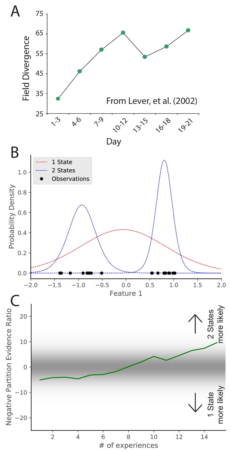
Learning to distinguish.
(A) Adapted from Lever et al., 2002, who compared place cell representations between alternating presentations of square and circle boxes. Field Divergence is expressed in percent and represents the fraction of place fields that remap between the two enclosures. The representations of the enclosures are initially similar, but diverge with learning. (B) Simulated observations (black dots) are generated from Gaussians centered at −1, 1. The model compares the posterior probability of the observations coming from one inferred hidden state (red) or two inferred hidden states (blue). (C) The relative probability assigned to the observations coming from two hidden states vs. one hidden state (Equation 7) is shown as a function of amount of experience. Early on, there is uncertainty about how many hidden states there are, whereas later two hidden states is more probable, similar to the empirical observations. As in Figure 2, values with a grey background can be thought of as partial remapping whereas values with a white background can be thought of as either complete remapping or lack of remapping depending on whether two states are more likely or one state is more likely. Note that the axis here has been flipped relative to Figure 2 in order to match the axis of the empirical results shown in panel A.
© 2002 Springer Nature. All rights reserved. Panel A is adapted from Lever et al., 2002 with permission (originally published as Supplementary Information Sheet 5). It is not covered by the CC-BY 4.0 licence and further reproduction of this panel would need permission from the copyright holder.
Figure 4
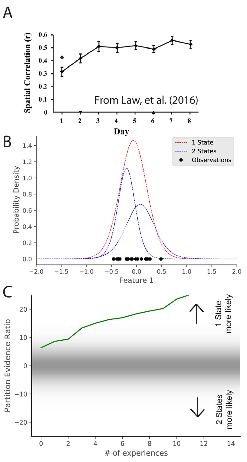
Map stabilization requires certainty about distributional statistics.
(A) Data from Law et al., 2016, showing the spatial correlation of the hippocampal map in repeated presentations of the same environment over multiple training days. Initially, the correlation is low, indicating extensive remapping between observations, but over the course of training the extent of remapping between observations decreases. (B) Observations (black dots) are generated from two Gaussians, both of which are centered at 0. The model compares the posterior probability of the observations coming from one inferred hidden state (red) or two inferred hidden states (blue). (C) The relative probability assigned to the observations coming from one hidden state vs. two hidden states (Equation 7) is shown as a function of amount of experience. Early in training, the two hypotheses have similar probabilities, whereas later one hidden state is overwhelmingly more probable. This corresponds to an increase in certainty over training, which would translate into a decreased tendency to remap, similar to the empirical observations. Note that the axis here has been flipped relative to Figure 3C in order to match the axis of the empirical results shown in panel A.
© 2016 Wiley Periodicals, Inc. All rights reserved. Panel A is reproduced from Law et al., 2016 with permission (originally published as Figure 2A). It is not covered by the CC-BY 4.0 licence and further reproduction of this panel would need permission from the copyright holder.
Figure 5
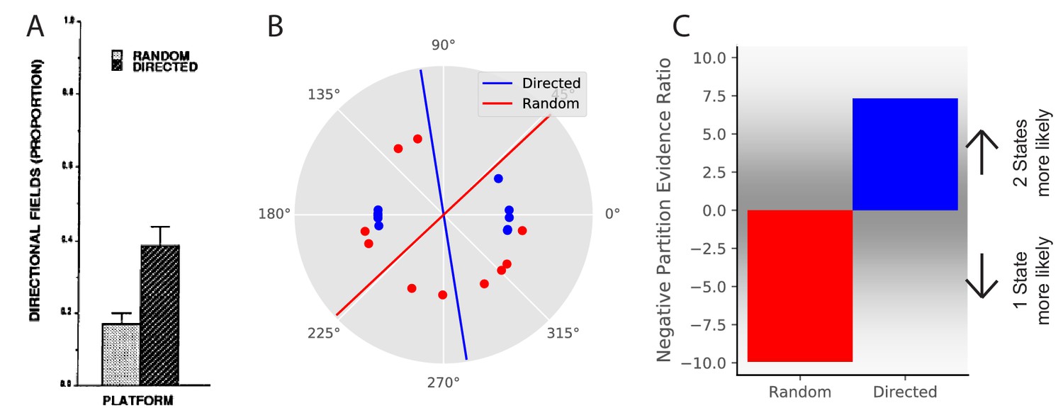
Place field directionality depends on statistics of behavior.
(A) Data from Markus et al., 1995, showing that place field remapping depends on the animal’s direction more when the animal is running in a stereotyped path than when the animal is running in random directions. (B) The model receives circular observations corresponding to the animal’s running direction. The model either receives observations drawn from a uniform distribution (red dots) or alternating from two Von Mises distributions with means of 0 and 180 degrees, and (blue dots). These observations are separated into two groups with a line that is the farthest from any observations (red and blue lines). (C) The partition evidence ratio between the hypothesis that all observations have been drawn from two hidden states separated by the lines in panel B vs. the hypothesis that all observations have been drawn from a single hidden state (Equation 7) after 10 observations. The model is more likely to put probability on the hypothesis that there are two hidden states when given the directional observations as opposed to the uniform observations. This is similar to the empirical results, where place fields are more likely to remap (more likely to infer two hidden states) when the animal is running in a directed fashion.
© 1995 Society for Neuroscience. All rights reserved. Panel A is reproduced from Markus et al., 1995 with permission (originally published as Figure 6A). It is not covered by the CC-BY 4.0 licence and further reproduction of this panel would need permission from the copyright holder.
Figure 6
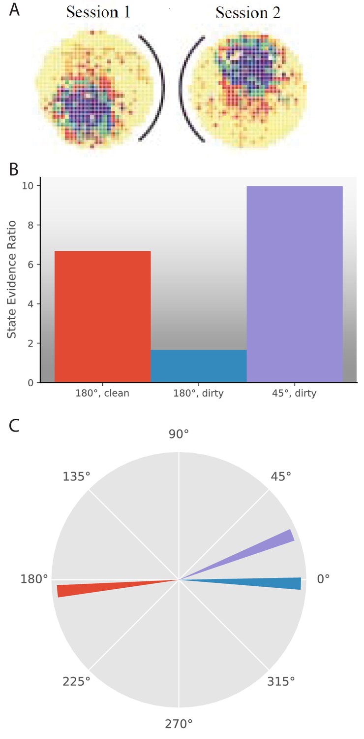
Response to cue rotation depends on experimental protocol.
(A) Data from Rotenberg and Muller, 1997. The black curve represents the location of the cue card. The heat map represents the firing rate of a given place cell. On rotation of the cue card by 180°, the place field is maintained, but rotated 180° with respect to the room reference frame. (B–C) Results of simulation of several experimental manipulations: In ‘180°, clean’, the cue card is rotated 180° while the animal is absent and the maze is cleaned before returning the animal. In ‘180°, dirty’, the cue card is rotated 180° while the animal is present and odor cues left by the animal are not removed. In ‘45°, dirty’, the cue card is rotated 45° while the animal is present and odor cues left by the animal are not removed. (B) The state evidence ratio is in favor of assigning to the same hidden state in all three manipulations. However, there is more uncertainty under the ‘180°, dirty’ manipulation. (C) The highest probability reference direction is depicted for each manipulation.
© 1997 The Royal Society (UK). All rights reserved. Panel A is reproduced from Rotenberg and Muller, 1997 with permission (originally published as parts of Figure 2A). It is not covered by the CC-BY 4.0 licence and further reproduction of this panel would need permission from the copyright holder.
Figure 7
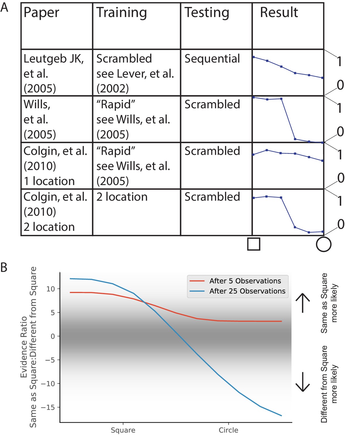
Morph experiments.
(A) Different experimental protocols give different results for the morph experiment. The results in the fourth column show the similarities in population representation of the intermediate morph shapes compared to the square shape. The results in the fourth column are adapted from the corresponding paper cited in the first column. All values are shown on a scale ranging from 0 to 1, where one is complete concordance of population representations and 0 is random concordance. We classify the results into two qualitative classes: the first and third rows have results where all levels of morph result in partial remapping, whereas the second and fourth rows switch between no remapping and complete remapping as morph level increases. Scrambling during testing does not seem to be related to this effect. Moreover, the same experimental protocol can have qualitatively different results in different labs (compare second and third rows). (B) We provide observations from two alternating Gaussians with means −1 and +1, just as in Figure 3. We test after 5 (red) or 25 (blue) training observations by providing intermediate values and measuring the relative probability of being assigned to the same hidden state as the −1 mean observations. We thus predict that both qualitative results can be achieved in the same lab simply by performing the morph testing at different points of training.
Figure 8
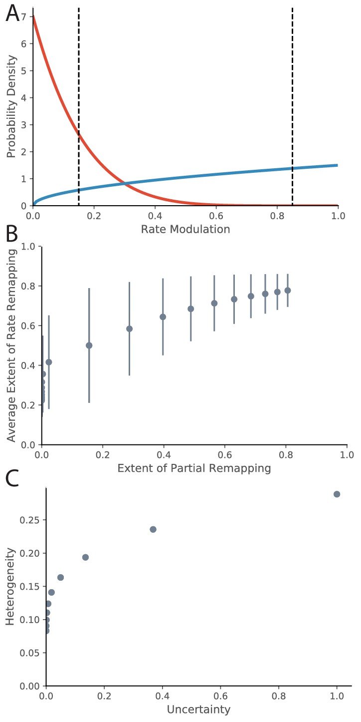
Relationship between Rate Remapping and Partial Remapping.
(A) The Beta distribution is used to illustrate the distribution in remapping responses over the place field population. Examples of the Beta distribution for parameter values (red) and (blue). We can draw a correspondence between the difference between these parameters and the evidence ratio. We can also characterize remapping behavior by saying that place fields with rate modulation less than the left-hand black dotted line do not remap, place fields between the black dotted lines rate remap, and place fields with rate modulation greater than the right-hand dotted black line completely remap. The extent of partial remapping would then be the fraction of cells that completely remap (fall to the right of the right-hand dotted black line). (B) The average extent of rate remapping has a positive relationship with the extent of partial remapping for a range of evidence ratios. Error bars are the standard deviation of the Beta distribution for those parameter values. (C) The amount of heterogeneity in rate remapping extents across the population of place fields has a positive relationship with the amount of uncertainty that the animal has over a range of evidence ratios.
Figure 9
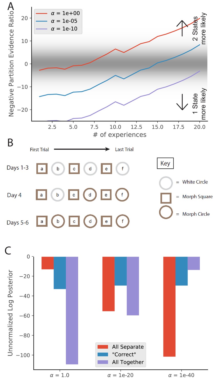
Animal-to-animal variability may be the result of animal-specific parameter settings.
(A) Simulations from Figure 3C with different values of . Larger values of alpha lead to a greater tendency to infer a larger number of hidden states, and therefore a faster transition from preferring the single-state model to the two-state model. (B) The training protocol from Supporting Figure 1C of Wills et al., 2005. (C) In red is the probability assigned to the hypothesis that the white circle, morph circle, and morph square are all generated by separate hidden states. In blue is the probability assigned to the hypothesis that the white circle and morph circle are generated by the same hidden state and the morph square is generated by a separate hidden state, which is the hypothesis that the authors expected. In purple is the probability assigned to the hypothesis that all of the enclosures are generated by the same hidden state (Equation 6). Different settings of result in different preferred assignments of observations to hidden states, corresponding to the finding that different animals had different remapping behaviors.
© 2005 AAAS. All rights reserved. Panel B is reproduced from Wills et al., 2005 with permission (originally published as Supporting Figure 1C). It is not covered by the CC-BY 4.0 licence and further reproduction of this panel would need permission from the copyright holder.
Figure 10
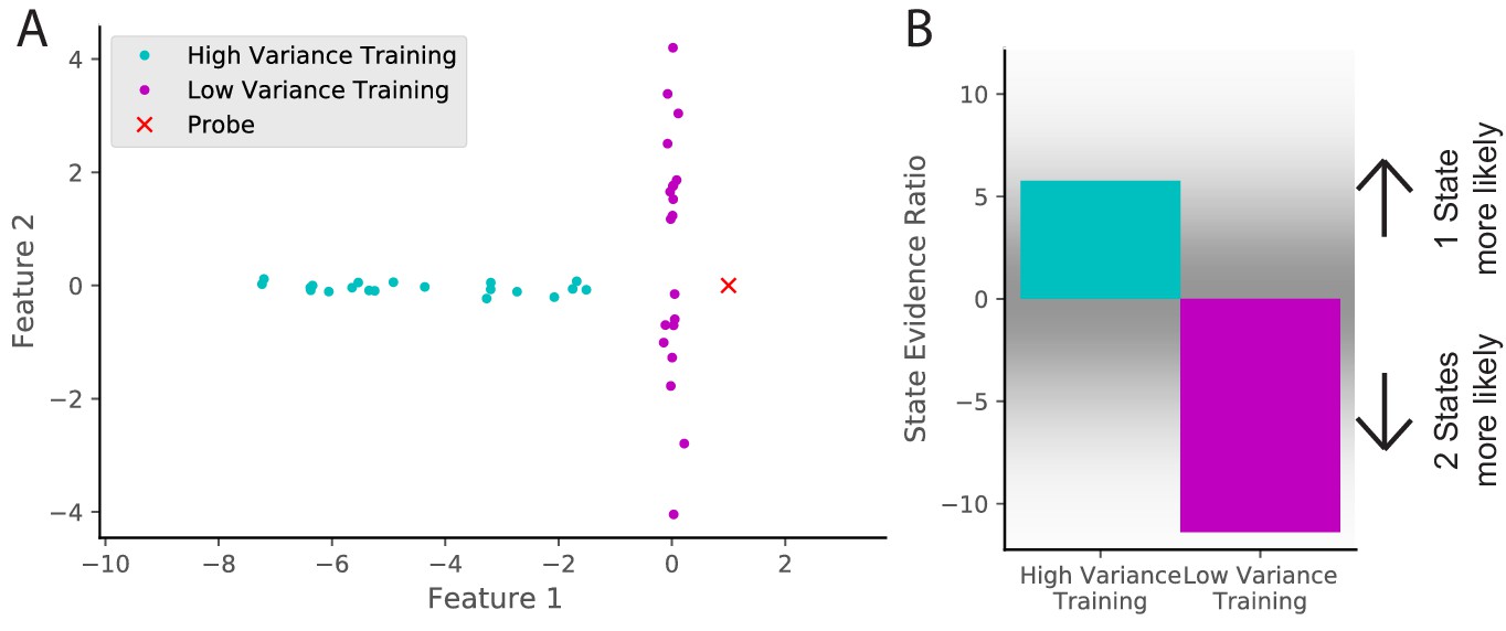
Cue variability should affect remapping behavior.
(A) Two training protocols (cyan and magenta) give (B) qualitatively different hidden state inferences when presented with the same novel observation (red dot in A). The cyan training is drawn from a Gaussian with mean [−5,0] and standard deviations [2, 0.1], whereas the magenta training is drawn from a Gaussian with mean [0,0] and standard deviations [0.1, 2]. The probe is presented after 20 training observations. The state evidence ratio here is the comparison between the assignment of the probe to the same hidden state as the training samples vs. a novel hidden state (Equation 11).
Additional files
Download links
A two-part list of links to download the article, or parts of the article, in various formats.
Downloads (link to download the article as PDF)
Open citations (links to open the citations from this article in various online reference manager services)
Cite this article (links to download the citations from this article in formats compatible with various reference manager tools)
Hippocampal remapping as hidden state inference
eLife 9:e51140.
https://doi.org/10.7554/eLife.51140


