Figures and data in Mitigating memory effects during undulatory locomotion on hysteretic materials

Figures
Tables
Additional files

14 figures, 4 tables and 1 additional file

Figures

Figure 1

Download asset Open asset

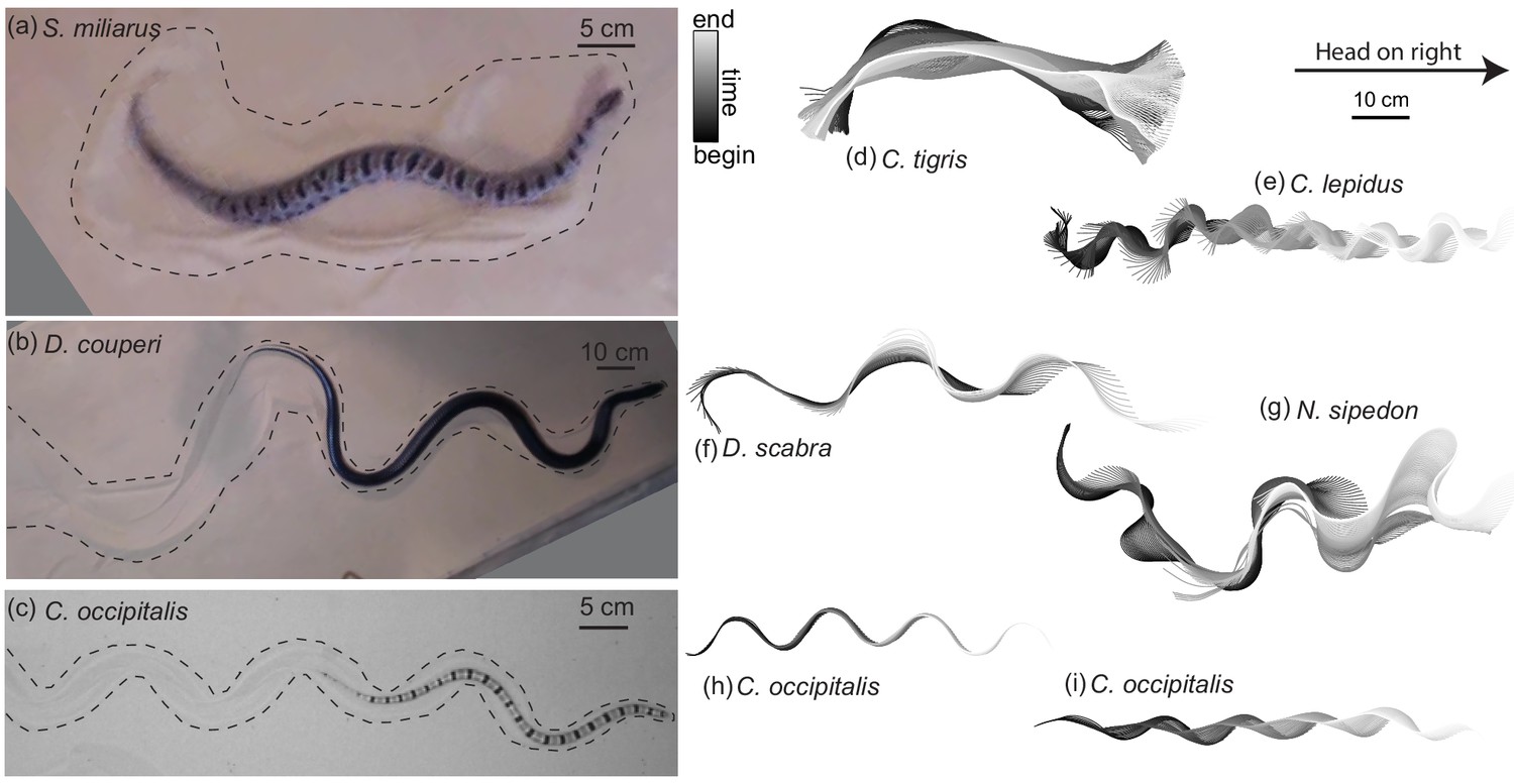
Body shape, waveform, and ability to progress across GM varies among snake species.

(**a–c**) Snapshots of snakes moving on the surface of GM. Dashed lines roughly indicate the area of material disturbed by the motion of the animal. (a) The generalist pygmy rattlesnake *Sistrurus miliarius* attempting to move on natural sand collected from Yuma, Arizona, USA. The animal has completed several undulations, sweeping GM lateral to the midline of the body. This snake failed to progress further than pictured. (b) The generalist eastern indigo snake *Drymarchon couperi*. On the same GM as (a) (c) The sand-specialist shovel-nosed snake *Chionactis occipitalis* in the lab on 300 μm glass particles. (**d–i**) Digitized midlines of animals. Color indicates time from beginning to end of the trial. All scaled to the 10 cm scale bar shown. (**d–g**) are on Yuma sand and (**h,i**) are on glass particles. (d) Tiger rattlesnake *Crotalus tigris*, a rocky habitat specialist. The animal was unable to progress on the GM. Total length of the trial $t_{t o t} =$ 25.7 s, time between plotted midlines $δ t = 100$ ms (e) Rock rattlesnake *Crotalus lepidus*, a rocky habitat specialist. $t_{t o t} =$ 9.4 s, $δ t = 33$ ms (f) Egg-eating snake *Dasypeltis scabra* inhabits a wide range of habitats in Africa. $t_{t o t} =$ 1.6 s, $δ t = 33$ ms (g) *Nerodia sipedon*, a water snake inhabiting most of the Eastern US extending into Canada. $t_{t o t} =$ 6.0 s, $δ t = 33$ ms (h) *C. occipitalis* 130 and (i) 128. These trials represent the inter-individual variation in kinematics. Some of the animals moved approximately ‘in a tube’ where all segments of the body followed in the path of their rostral neighbors (e.g. (h), $t_{t o t} =$ 1.25 s, $δ t = 12$ ms) while others used this strategy only on the anterior portion of the body, appearing to drag the posterior segments in a more or less straight line behind themselves (e.g. (i), $t_{t o t} =$ 1.01 s, $δ t = 12$ ms).

Figure 2 with 2 supplements

Download asset Open asset

Snake waveform parameters measured in experiment.

(a, *left*) $θ = acos (\hat{x} \cdot \hat{t})$ for local tangent angle, $\hat{t}$ and average direction of motion $\hat{x}$ . Example body posture shown, colored by $θ$ . (a, *right*) Example serpenoid curves (Equation 1) of different $ξ$ on a body of fixed length and $θ_{m} = 48$ deg. (b) *C. occipitalis* experimental measurements plotted in the $(θ_{m}, ξ)$ parameter space. Color indicates animal number. Markers are the mean and range of each individual taken over all trials. N = 9 individuals, n = 30 trials. The gray region in the upper right corner are waves which are inaccessible given the flexibility of the snake (Sharpe et al., 2015). $θ_{m}$ was comparable to values measured from images of tracks taken in the field (Figure 2—figure supplement 2). (*inset*) A close-up of the data with mean and range from each trial plotted individually. Color consistent with the main plot (Linear fit with 95% confidence interval to inset data: slope −0.016 (-0.020,–0.011) intercept 2.66 (2.42, 2.90), R-square = 0.6). (c) Axes as in (b), black cross is the combined *C. occipitalis* measurements. Colored crosses are the mean and range of values measured on a per-trial basis in the non-sand-specialists, different species indicated by color. N = 22 individuals, n = 38 trials.

Figure 2—figure supplement 1

Download asset Open asset

Principal component analysis (PCA) of all sand snake shapes.

(a, *top*) Tangent angle, $θ$ is the angle between $\hat{t}$ and the average direction of motion of the animal, $\hat{x}$ . (*bottom*) Example space-time plot of $θ$ , corresponding to the *bottom* trial in c. The diagonal bands indicate a head-to-tail traveling wave propagated at constant speed. (b) The two dominant PCs representing $θ$ . The solid lines are the experimental results, the dashed lines are sine fits to $A_{i} sin (ξ_{i} s + ϕ_{i})$ . Coefficients with 95% confidence bounds were $A_{1} = 0.83 (0.82, 0.84)$ , $A_{2} = 0.92 (0.90, 0.94)$ , $ξ_{1} = 1.44 (1.43, 1.45)$ , $ξ_{2} = 1.40 (1.39, 1.41)$ , $ϕ_{1} = 0.05 π (0.04 π, 0.06 π)$ , $ϕ_{2} = - 0.41 π (0.42 π, 0.39 π)$ . Both vectors were divided by the same maximum value such that the maximum amplitude was one. These two PCs account for 91% of the variance. (c) The amplitudes $α_{1}$ and $α_{2}$ associated with the PCs in e. Color indicates the frame number for all trials (N = 9, n = 30) combined. The trajectories move counterclockwise around the circular structure, indicating a traveling wave. The radius of this circle is the amplitude of the wave of $θ$ . See Stephens et al., 2008.

Figure 2—figure supplement 2

Download asset Open asset

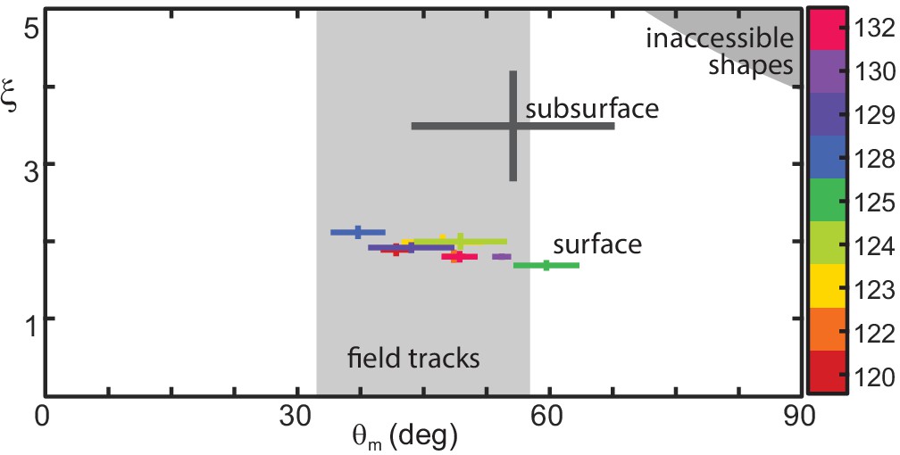
Kinematics of *C. occipitalis* compared to field measurements.

(Plot as in main text with field measurements added). The light gray rectangle illustrates the range of $θ_{m}$ measured from photographs taken of *C. occipitalis* tracks found in the desert (17 measurements). Experimental measurements plotted in the ${θ_{m}, ξ}$ parameter space. Color indicates animal number. Markers are the mean and range of each individual taken over all trials. N = 9 individuals, 30 trials. The gray cross is the waveform used by *C. occipitalis* when moving subsurface. The surface waveform was distinct from that used by this species when moving buried within the GM (Sharpe et al., 2015). While the angular amplitude was not significantly different (subsurface $θ_{m} = 54.7 \pm 11.9$ deg compared to the surface value $θ_{m} = 48.3 \pm 7.0$ deg for all snakes combined, 2-tailed t-test $P = 0.04$ mean of all trials and std of mean of all trials), the value of $ξ$ was less for surface swimming ( $ξ = 3.53 \pm 0.85$ subsurface versus $ξ = 1.90 \pm 0.14$ at the surface, P < 0.001). The gray region in the upper right corner are waves which are inaccessible given the flexibility of the snake (Sharpe et al., 2015).

Figure 3 with 1 supplement

Download asset Open asset

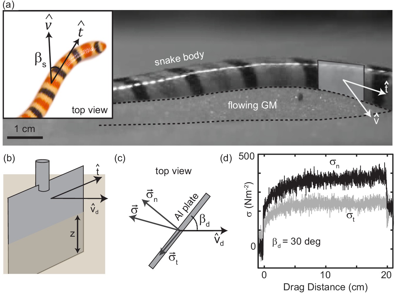
Characterizing granular forces experienced by snakes by empirically measuring stress on a partially buried plate.

(a) Side-view of *C. occipitalis* moving on the surface. Snake is moving from left to right. The surface was initially featureless, the piles of sand outlined by the black, dashed line were generated by the motion of the snake. Gray rectangle illustrates the flat plate snake body segment model, aligned with $\hat{t}$ of the midline moving in direction $\hat{v}$ . (*inset*) Top view of a snake. $β_{s}$ is the angle between the local tangent and velocity unit vectors. (b) Aluminum plate, dimensions 3 × 1.5 × 0.3 cm³. The plate was kept at a constant depth, $z$ , from the undisturbed free surface of the GM to the bottom of the intruder. (c) Top view of the plate moving in a direction $\hat{v_{d}}$ at angle $β_{d}$ . Components $σ_{t}$ and $σ_{n}$ of the total stress, $σ$ . (d) Raw drag data collected at $β_{d} = 30$ deg and $v_{d} = 10$ mm s^-1 as a function of drag distance of the plate. The upper black curve is $σ_{n}$ , the lower gray is $σ_{t}$ . Force data collected at 1000 Hz, plotted here down-sampled by a factor of 10 to facilitate rendering.

Figure 3—video 1

Download asset

posterframe for video — Side view of *C. occipitalis* moving on GM.

Video is slowed ten times.

Figure 4 with 2 supplements

Download asset Open asset

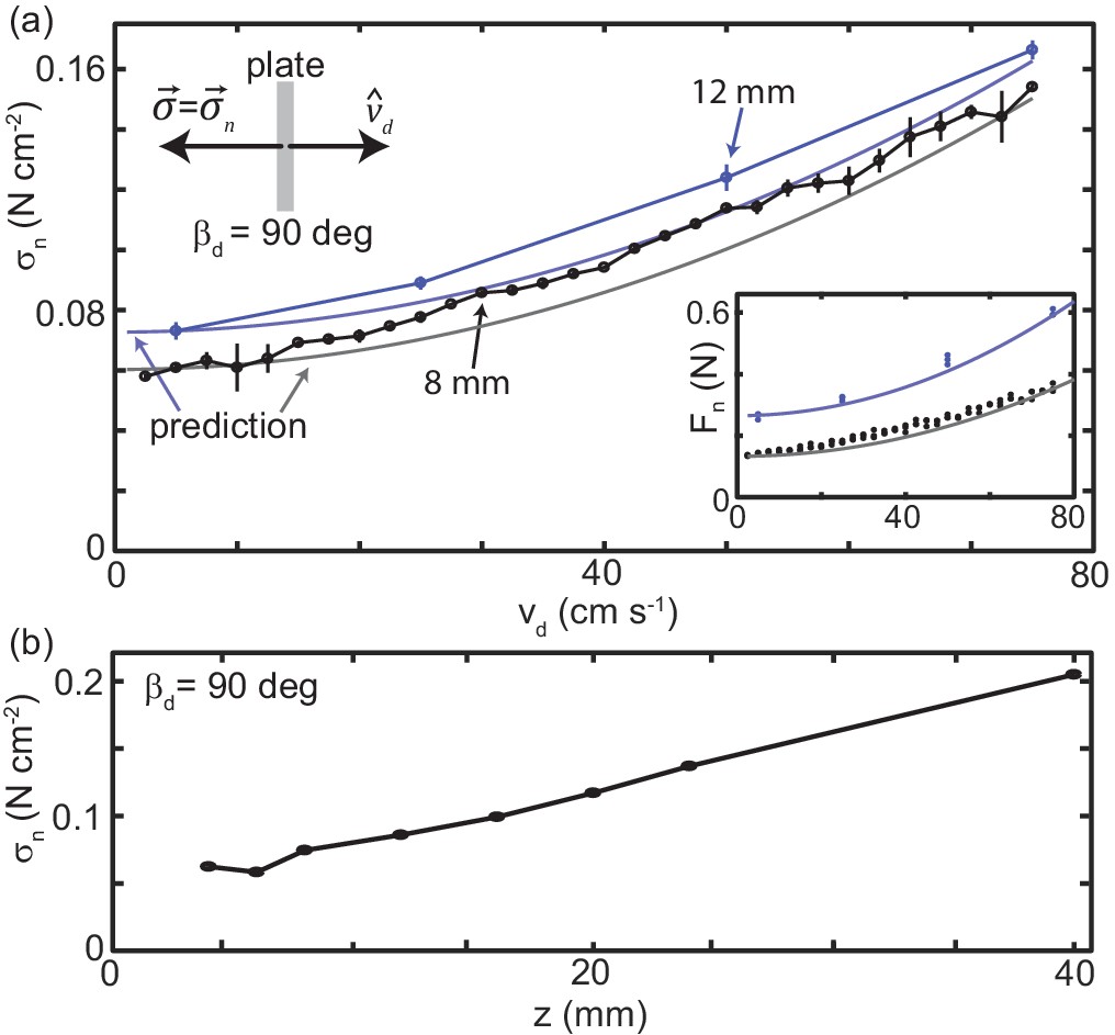
Granular drag stress as a function of speed and depth.

(a) Stress normal to the plate face as a function of $v_{d}$ at a constant depth $z = 8$ mm (black points) and $z = 12$ mm (blue points). As shown in the diagram at the upper left, $β_{d} = 90$ deg for all trials such that the total stress was equal to $σ_{n}$ . Markers are mean and std. of three trials. Where error bar is not visible error is smaller than the marker. Gray curve is the model prediction for $z = 8$ mm and light blue curve for $z = 12$ mm. (*inset*) Normal force versus $v_{d}$ measured in experiment (circle markers) and as predicted by the model (solid curves). Color is consistent with the main plot. Each dot is the average force measured in one trial, all trials shown. (b) Stress normal to the plate face as a function of $z$ at $v_{d} = 10$ mm s^-1. All experimental data shown in this figure are averaged from 10 to 20 cm drag distance. Over this distance the force had reached steady state and the robot arm was moving at the commanded velocity.

Figure 4—figure supplement 1

Download asset Open asset

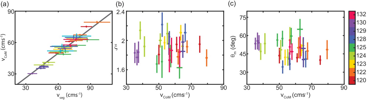
*C. occipitalis* movement speed independent of waveform parameters.

(a) Center-of-mass velocity, $v_{C o M}$ , versus segment velocity (as if one were riding on the body), $v_{s e g}$ . Lines are mean and std. of each measurement. Each data point is an individual trial, individual number as shown in colorbar to the far right. Colors are consistent with those in main text Figure 2. Gray line is the linear fit (mean and 95% confidence intervals of slope = 0.81 (0.74, 0.89), y-intercept = 0.67 (-4.63 5.94), R-squared = 0.94, RMSE = 2.88) N = 9 individuals, n = 30 trials. (b) Number of waves on the body, $ξ$ , versus $v_{C o M}$ . Mean and std. for each trial, colored according to individual. (c) Attack angle, $θ_{m}$ , versus $v_{C o M}$ . Mean and std. for each trial, colored according to individual.

Figure 4—figure supplement 2

Download asset Open asset

*C. occipitalis* tracks.

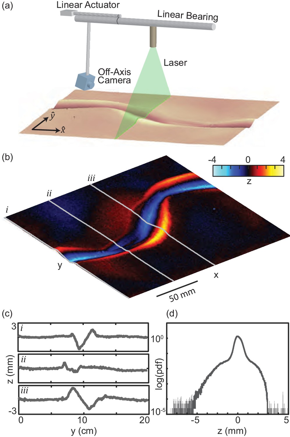
(a) Diagram of the laser-line apparatus. A laser sheet spans the sand-fluidized bed. An off-axis camera (Logitech C920 HD Pro Webcam) captured images of the laser line. Both the laser and camera were affixed to a linear bearing and moved using a linear actuator (Firgelli). We used MATLAB to move the actuator and collect an image every 1 mm, verified using a ruler placed in view of the camera. The location of bright pixels in the images was used to estimate the height of the material at that x location as a function of y. (b) Track in the GM remaining after a trial. Warm colors indicate the piles formed rising above the free surface. The snake travelled in the direction indicated. The body intrudes beneath the free surface and yields the material, creating piles on the anterior edges of the path like those described by Mosauer, 1933 and seen in the tracks observed in the field. (c) Height of the material as a function of y at three x locations, i, ii, and *iii* as shown in (b). (d) Log of the probability density function of all z measurements shown in (b). The free surface is at zero.

Figure 5

Download asset Open asset

Stress as a function of plate drag angle.

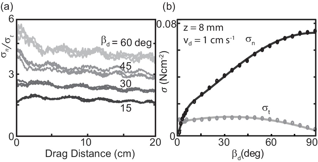
(a) Stress anisotropy versus drag distance. Since $σ_{t}$ is small, values with noise included can approach zero. As we were interested in the force evolution over several cm (for the plotted drag speed this corresponds to signals $< 1$ Hz), we removed fluctuations above 5 Hz using a low-pass butterworth filter. Curves from three trials are shown for each of four different, fixed $β_{d} = 15$ (darkest, bottom curve), 30, 45, and 60 deg (lightest, top curve) as labeled on the right of the plot. The slopes of a linear regression fit to the average of three trials as a function of drag distance were −1.8 × 10^-5, −2.9 × 10^-5, −5.0 × 10^-5 and −6.4 × 10^-5 cm^-1 for $β_{d} =$ 15, 30, 45, and 60 deg, respectively (R-square = 0.6, 0.8, 0.8, and 0.7). (b) Average stress as a function of changing drag angle. Each measurement was calculated by averaging the raw stress data from 10 to 20 cm drag distance. Each data point is the mean and standard deviation of three trials; error bars are smaller than the markers. Solid lines are the fit functions used in the RFT calculations.

Figure 6

Download asset Open asset

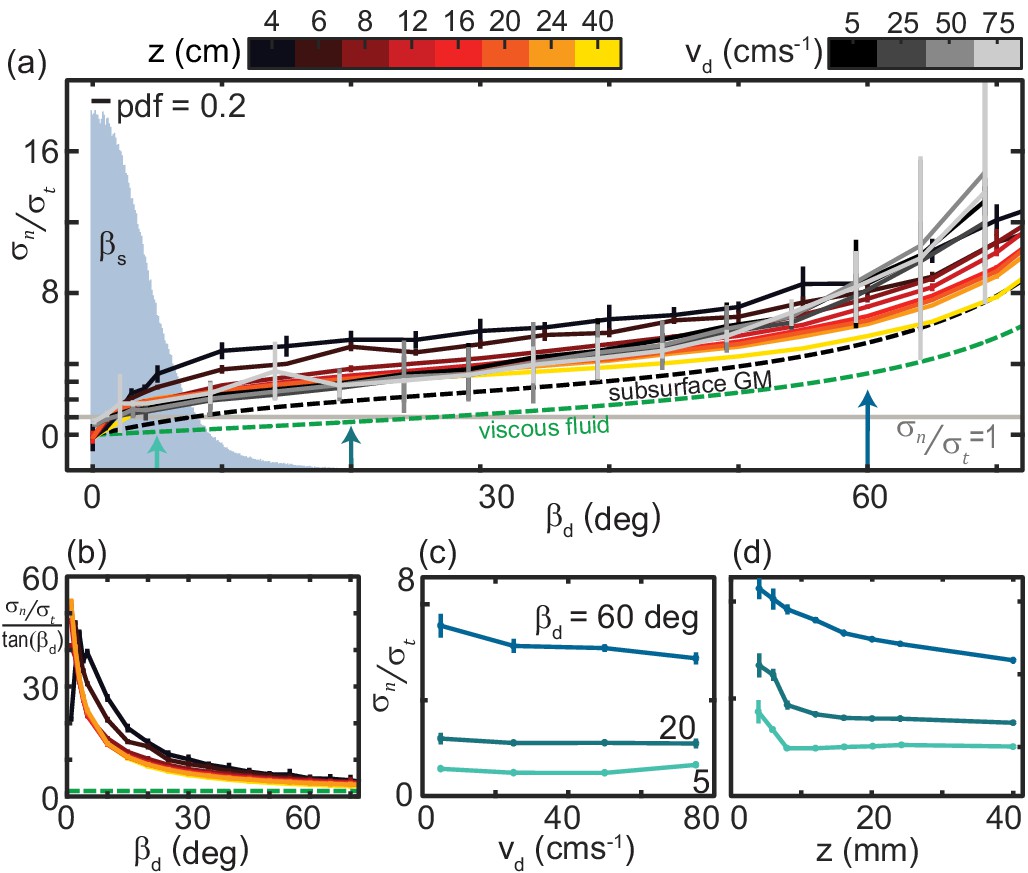
The ratio of granular normal to tangential stress, $σ_{n} / σ_{t}$ , is not strongly dependent on speed or depth.

(a) $σ_{n} / σ_{t}$ as a function of $β_{d}$ . Light gray horizontal line indicates $σ_{n} / σ_{t} = 1$ . All depths and speeds are plotted as indicated by color. Dashed curves are the anistropy for a low-Re swimmer in Newtonian fluid (green, $C_{n} / C_{t} \approx 1.5$ for a smooth, long, and slender swimmer Boyle, 2010) and subsurface in the same ≈ 300 µm GM used in this study (black). Labels are below the associated curves. The solid gray area is the probability density (pdf) of $β_{s}$ measured on the snake in experiment (N = 9 individuals, n = 30 trials). (b) $\frac{σ_{n} / σ_{t}}{tan (β_{d})}$ versus $β_{d}$ for the surface granular drag at varying $z$ and viscous fluid shown in (a). Line color and types consistent with (a). (c) $σ_{n} / σ_{t}$ as a function of $v_{d}$ at the values of $β_{s}$ indicated. Colors correspond to the colored arrows on the horizontal axis in (a). Linear fits to the data (not shown) with slope, m, and 95% confidence bounds in parentheses for $β_{d} = 60$ deg $m = - 0.019$ deg (−0.040,0.003) R-square = 0.88; $β_{d} = 20$ deg $m = - 0.003$ deg (−0.007, 0.002) R-square = 0.75; $β_{d} = 5$ deg $m = 0.003$ deg (−0.011, 0.016) R-square = 0.23, (d) $σ_{n} / σ_{t}$ as a function of $z$ . Colors and angles are the same as in (c).

Figure 7 with 1 supplement

Download asset Open asset

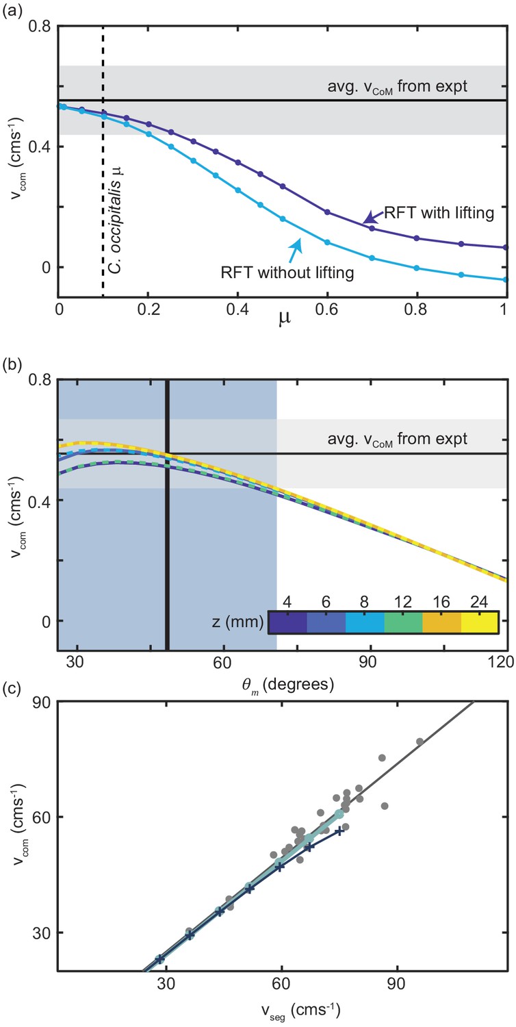
Comparison of RFT results with snake performance.

(a) $v_{C o M}$ as a function of the animal scale-grain friction. μ = 0.1 corresponding to *C. occipitalis* is indicated by the vertical dashed line. The light blue curve is RFT calculation for the snake parameters without any lifting and the dark blue curve was calculated for lifting of segments whose $θ$ was in the lowest 41% (equivalent to the wave apexes Figure 7—figure supplement 1). The horizontal black line and gray bar are the average and range of $v_{C o M}$ calculated from experiment. (b) RFT calculation of $v_{C o M}$ as a function of $θ_{m}$ using granular force relations measured at different depths, $z$ , denoted by color. Three of the curves are dashed so that all six curves can be seen. The vertical line and blue bar denote the mean and range of $θ_{m}$ measured in experiment. (c) Relationship between $v_{C o M}$ and $v_{s e g}$ measured in *C. occipitalis* experiment (gray circles) and predicted by RFT using force relations measured at $z = 8$ mm for constant $v_{d} = 10$ mm s^-1 (light blue line) and $v_{d} = v_{s e g}$ (dark blue line and cross markers). Solid gray line is a linear fit to the animal data $v_{C o M} = 0.82 v_{s e g} + 0.54$ (R-square = 0.94).

Figure 7—figure supplement 1

Download asset Open asset

Measurement of the vertical wave of lifting.

(a) An OptiTrack motion capture system (four Prime 17W cameras) captured 3D kinematics of *C. occipitalis* moving in the fluidized track way by tracking 3 mm diameter IR-reflective markers placed at 1.5 cm intervals along the mid-line. Space-time plot of $θ$ is the fractional arclength from the neck at $s = 0$ to the vent at $s = 1$ . (b) Space-time plot of the vertical position of the snake's midline measured relative to the free surface. Axes are as in (a). (c) Probability density of the wavenumber of the horizontal wave (gray) and vertical wave (red). The ratio of the median values of the two curves is 2.1, indicating that the spatial frequency of the wave of lifting is twice that of the wave in the horizontal plane. There were some outliers due to measurement error which were $ξ > 10$ that have been excluded as unphysical. (d) The phase of the wave in $z$ versus the wave in $θ$ . The wave in $z$ is traveling at twice the frequency of that in $θ$ . The result is that the peaks of the wave in $z$ align with the extrema in $θ$ , that is, the apexes of the horizontal wave are lifted off of the substrate. N = 3 individuals (122–11 trials, 124–3 trials, 131–3 trials). Ratio of the median values of each curve is 2.1. (e) Diagram of the lifting used in RFT calculation. Shown is an example serpenoid curve of the average waveform measured in experiment. The CoM position of each of the 100 segments used in the calculation are displayed as circles, colored by whether they are in contact with the substrate (gray) or lifted (red, force set to zero).

Figure 8 with 1 supplement

Download asset Open asset

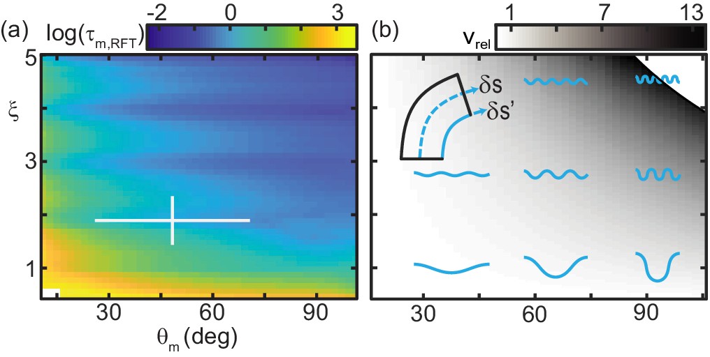
Trade-off between external torque and internal actuation speed.

(a) RFT prediction of the peak joint level torque, $τ_{m, R F T}$ , occurring during one undulation cycle as a function of $θ_{m}$ and $ξ$ . Color indicates the log of $τ_{m, R F T}$ . White cross is the mean and range of animal $θ_{m}$ and $ξ$ . measured in experiment. (b) Heatmap of relative actuation speed, $v_{r e l} = \frac{v_{s h o r t, o} - v_{s h o r t} (θ_{m}, ξ, f)}{v_{s h o r t . o}}$ at the nominal waveform of *C. occipitalis* ( $θ_{m} = 48.4$ , $ξ = 1.9$ ). Frequency, $f$ , is calculated to yield the desired $v_{C o M}$ for a given waveform’s stride length (see Materials and methods for details). Diagram in upper left corner illustrates the bending beam. The nominal length of a segment at the midline is $δ s$ , blue dashed line. The length of the inside of a segment is $δ s^{'}$ , solid blue line. Relative actuation speed is the rate of change of $δ s^{'}$ at the nominal $v_{C o M}$ , assuming no-slip motion.

Figure 8—figure supplement 1

Download asset Open asset

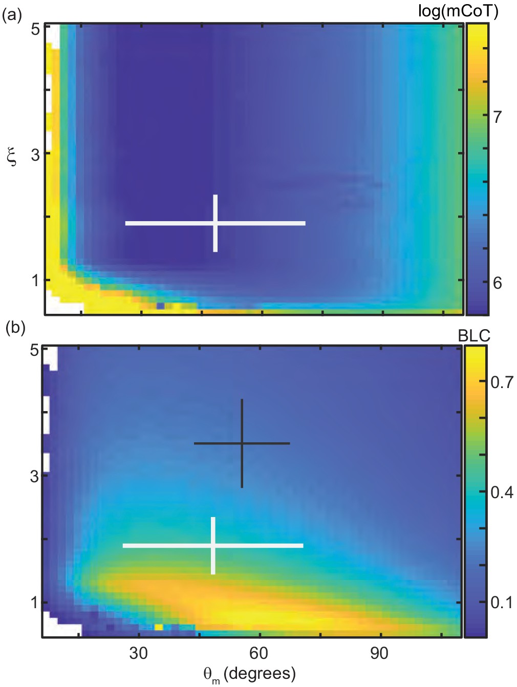
Surface RFT results for mCoT, BLC, and $τ_{m, R F T}$ .

The horizontal axis of all plots is $θ_{m}$ . Moving from left to right increases the amplitude of the body wave.Moving from left to right increases the amplitude of the body wave. The vertical axis is $ξ$ , the number of waves on the body increases from bottom to top of each plot. White crosses are average ± range of mean values measured in 30 snake trials (N = 9 individuals). (a) Mechanical cost of transport, mCoT, calculated for each pair of $θ_{m}$ and $ξ$ . The color corresponds to log(mCoT). (b) Bodylengths traveled pedr cycle, BLC. Black cross is the waveform used by *C. occipitalis* when moving subsurface within the same ≈ 300 μm glass particles. Values from Sharpe et al., 2015.

Figure 9

Download asset Open asset

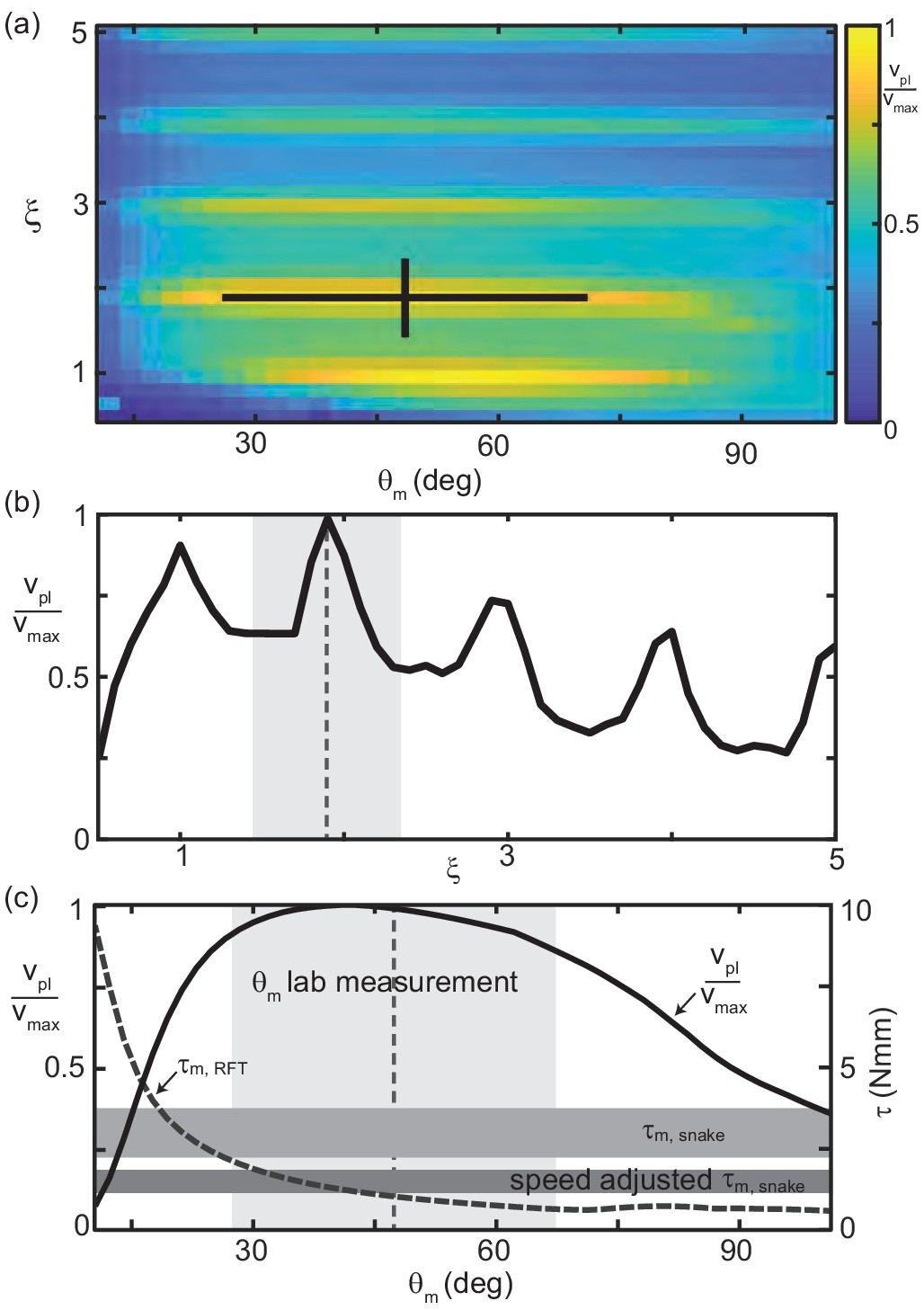
RFT reveals waveform balances internal and external concerns in *C. occipitalis*.

(a) Segment-power-limited velocity, $v_{p l}$ , divided by $v_{m a x}$ , the largest value of $v_{p l}$ , in the $θ_{m}$ , $ξ$ space. Black cross is the snake waveform as in (Figure 2(c)). (b) $v_{p l} / v_{m a x}$ versus $ξ$ for $θ_{m} = 48.4$ deg, the average experimental value. This is a vertical slice of (a). The vertical dashed line and gray shaded area are the mean and range of snake $ξ$ values. (c) Solid black curve $v_{p l} / v_{m a x}$ (left vertical axis) and gray dashed curve $τ_{m, R F T}$ (right vertical axis) versus $θ_{m}$ for $ξ = 1.90$ (the average snake value) are horizontal slices of (a) and Figure 8(a), respectively. The vertical dashed line and light gray shaded area are the mean and range of snake $θ_{m}$ . Horizontal gray bars are the estimated muscle torque capabilities of the snakes (see Materials and methods for details). The upper bar, $τ_{m, s n a k e}$ is the estimated maximum muscle torque and the bottom bar, speed adjusted $τ_{m, s n a k e}$ , is the maximum torque reduced to reflect the average muscle shortening speed of the snakes at the average experimentally measured velocity.

Figure 10 with 2 supplements

Download asset Open asset

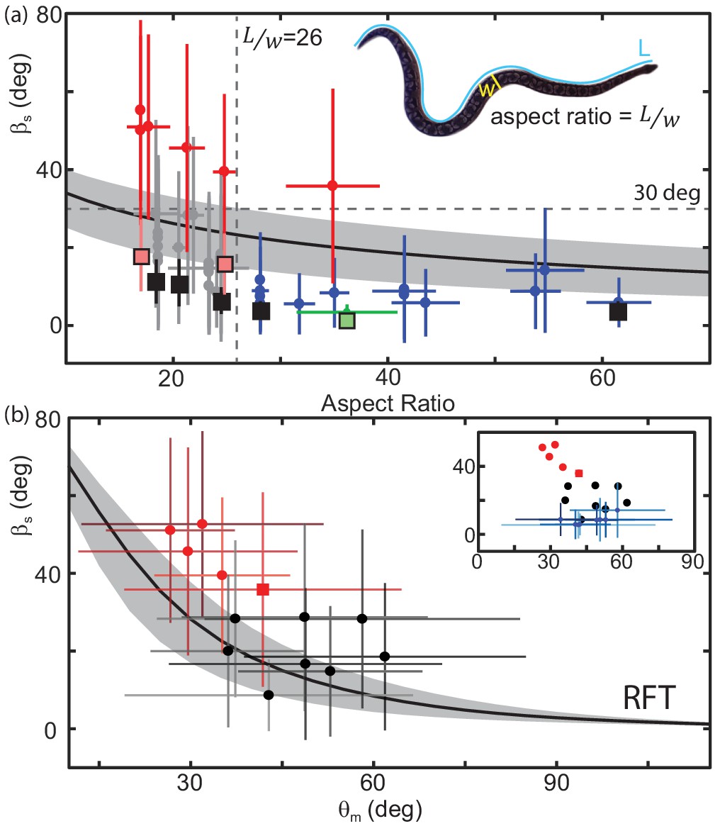
Performance depends on aspect ratio and waveform.

(a) Slip as a function of aspect ratio, $L / w$ as illustrated on the snapshot of a snake (*Acrantophis dumerili*, $L / w = 23.2$ ) where $L$ is the total length of the snake (blue curve) and $w$ is the width at the widest point (yellow line). Circle markers and vertical lines indicate the mean and std. of each trial. Horizontal bars are the range of aspect ratios measured from video stills by two different researchers. Black are successful trials, red are failures, green is *C. occipitalis*. Each animal tested had a unique aspect ratio; for the non-sand-specialists, multiple data points at the same $L / w$ indicate multiple trials for the same animal. N = 22 animals, n = 38 trials. Only mean shown for *C. occipitalis* (N = 9, n = 30). Black curve is the RFT estimation of slip using a scale friction of μ = 0.15. Gray area indicates predictions for μ = 0.1 (lower slip) and 0.2 (higher slip). Square markers indicate RFT prediction of slip for that animal using a scale friction of μ = 0.15 with vertical lines showing range from μ = 0.1 to 0.2. For *C. occipitalis* μ = 0.1 (Sharpe et al., 2015) and min/max = 0.05/0.15. All RFT predictions used force relations for 300 µm glass beads assuming intrusion depth of 8 mm. (b) Slip versus $θ_{m}$ for animals with $L / w < 26$ . Mean and standard deviation of all measurements in a trial. Square marker is the snake $L / w > 26$ which failed. If an animal performed more than one trial we combined the measurements of all trials before taking the mean and std. dev. Successful trials in black, failures in red. Black curve is the RFT prediction using the average waveform and anatomy values calculated using all species studied, $ξ = 2.5$ , mass = 0.63 kg, L = 89 cm, and an estimated scale friction of μ = 0.15. Gray band indicates predictions for friction μ = 0.1 and 0.2. (*inset*) Black and red circles are the averages from the main plot. Blue markers are successful trials $L / w > 26$ .

Figure 10—figure supplement 1

Download asset Open asset

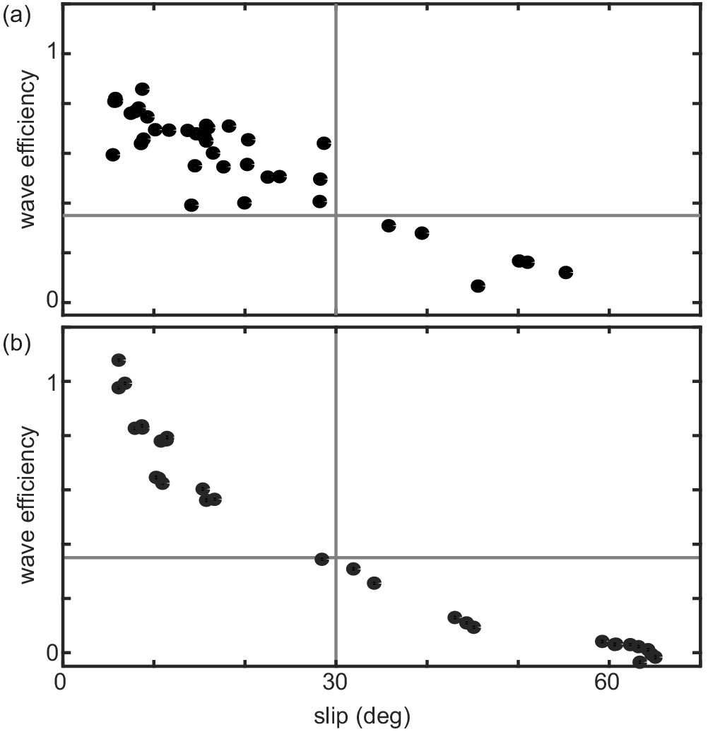
Wave efficiency versus slip.

(a) Wave efficiency, average distance traveled in one undulation cycle divided by the average wavelength, as a function of slip. Black markers are from each experimental trial taken using the various snake species on natural sand. Vertical gray line is at $β_{s} = 30$ deg and horizontal line is at wave efficiency of 0.35. (b) Wave efficiency of the robot, distance traveled in one undulation cycle (calculated as the total distance traveled divided by three) divided by the wavelength, as a function of slip. Black markers are from each experimental trial taken using the robot for all trials wavenumber 1, 1.2, and 1.4. Vertical gray line is at $β_{s} = 30$ deg and horizontal line is at wave efficiency of 0.35.

Figure 10—figure supplement 2

Download asset Open asset

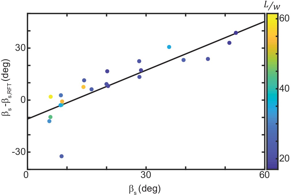
Slip measured in experiment versus RFT prediction.

Horizontal axis is the average slip measured in experiment. For animals with more than one trial the mean of the averages is plotted. Vertical axis is the difference between slip measured in experiment and that estimated using RFT and that individual’s parameters (mass, length, average wavenumber, and average attack angle). Points colored by aspect ratio. Black line is a linear fit, $R^{2} = 0.75$ .

Figure 11

Download asset Open asset

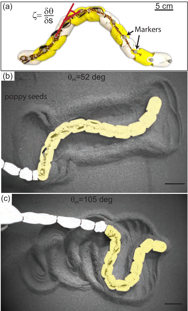
Systematic exploration of substrate memory effects using a robophysical model.

(a) The 10 joint, 11 segment robot constructed using ten Dynamixel AX-12A servo actuators (Robotis) with a stall torque of 15.3 kg·cm. Yellow and white segments are 3D printed cylindrical casings, each housing one motor. Length = 72 cm and $L / w = 11.3$ . (**b,c**) Stills of the robot taken after it has completed 2.75 undulation cycles. $θ_{m} = 52$ deg in (b), $θ_{m} = 105$ deg in (c), and $ξ = 1$ in both cases. Robot is artificially colored yellow to distinguish the body from the tail cord in white. Note the large appearance of the tail cord in c is due to perspective as the researcher was standing and loosely holding the cord above the substrate.

Figure 12

Download asset Open asset

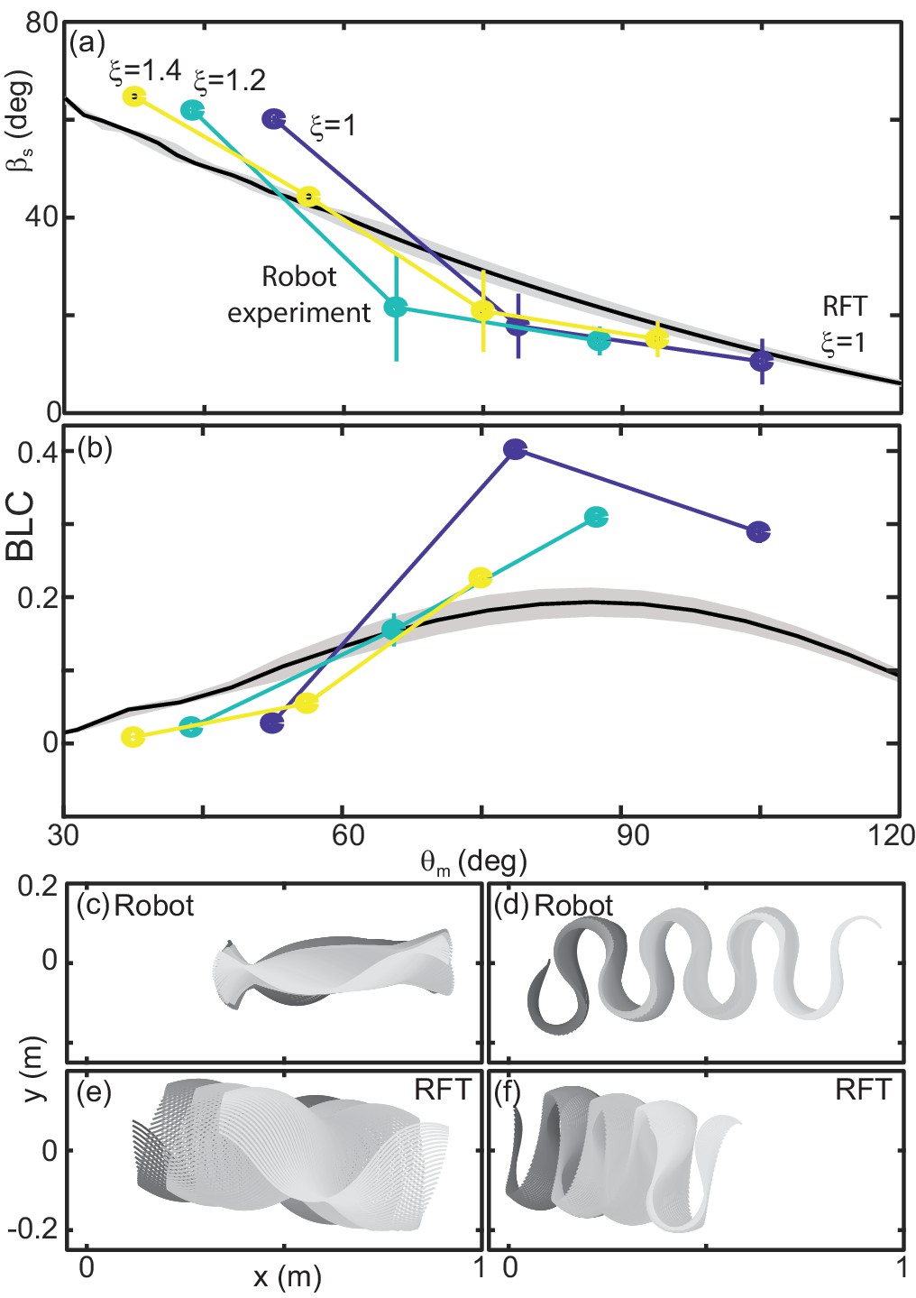
Robot performance is sensitive to the waveform and poorly predicted by RFT.

(a) Slip versus $θ_{m}$ . Robot measurements are circles connected by solid lines. $ξ$ is indicated by color, yellow is 1.4, teal is 1.2, and blue is 1. Mean and std. of three trials. Where error bars are not visible they are smaller than the marker. RFT prediction is the solid black curve. The gray shaded region indicates uncertainty in our knowledge of the robot’s mass (because of the weight of the tail cord which is held above the substrate) and friction coefficient. (b) Body lengths traveled in a single undulation cycle (BLC) as a function of attack angle. Colors and lines are consistent with (a). (**c,d**) Robot and (**e,f**) RFT predicted kinematics for $ξ = 1$ . Color indicates time from the beginning to the end (darker to lighter gray). Both robot and RFT trajectories include three complete undulations. (**c,e**) $θ_{m} = 52$ deg. (**d,f**) $θ_{m} = 105$ deg.

Figure 13 with 3 supplements

Download asset Open asset

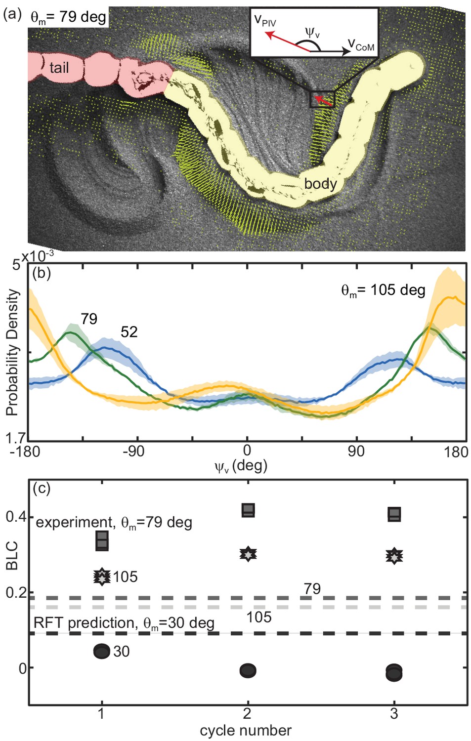
Material remodeling determines kinematics of the robot.

(a) Snapshot of the robot moving on poppy seeds with grain velocity vectors estimated using PIV shown in yellow. We measured the grain velocity vector angle, $ψ_{v}$ as shown. A mask of the body (yellow) and tail (red) was used in all PIV calculations and vectors both too close and too far from the body were not included in calculating $ψ_{v}$ . Vectors shown are representative of those included. We collected three trials per condition and three complete undulation cycles per trial. (*inset*) Diagram of $ψ_{v}$ for an example estimated grain velocity vector in red. $v_{C o M}$ is pointing in the average direction of motion of the robot. (b) Probability density of $ψ_{v}$ for each of the three $θ_{m}$ tested, $θ_{m} = 105$ (yellow), 79 (green), and 52 (blue) as labelled on the plot. Curves were calculated using all $ψ_{v}$ measured in space and time in a single trial. Solid lines are the average curve and the shaded area indicates the standard deviation across the three trials. (c) Distance traveled by the robot in a single step, normalized by body length, measured at the end of each of three consecutive undulation cycles. $ξ = 1$ for all trials shown. From darkest to lightest gray color: circles are $θ_{m} = 30$ deg, square are 70 deg, and stars are 105 deg. Three trials are plotted separately for each step. RFT prediction shown as a horizontal lines with color corresponding to experiment.

Figure 13—video 1

Download asset

Figure 13—video 2

Download asset

Figure 13—video 3

Download asset

Figure 14

Download asset Open asset

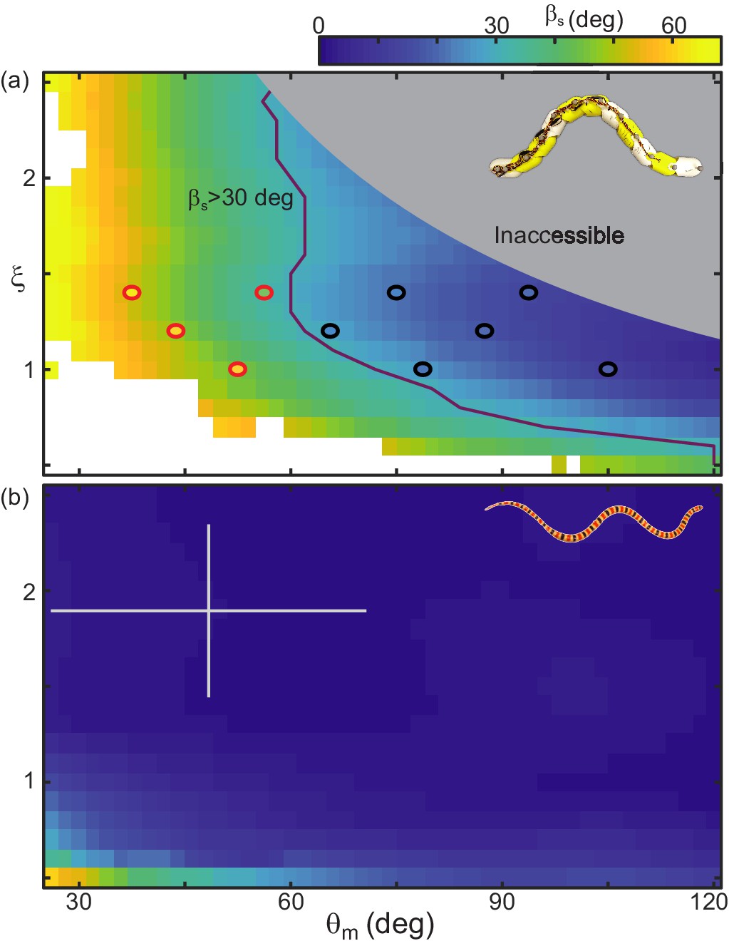
RFT prediction of slip gives a heuristic for performance.

(a) Color denotes slip as $θ_{m}$ and $ξ$ vary, calculated using RFT for robot dimensions and poppy seed force relations. Circles indicate the parameter combinations tested on the robot. Waveforms which were successful over three undulations are black, red markers denote unsuccessful parameters (distance per undulation over wavelength <0.35, Figure 10—figure supplement 1). Purple line indicates where RFT predicts $β_{s} \approx 30$ deg. The lightly shaded region denotes waveforms which the robot cannot perform. White areas indicate where the RFT calculation did not converge on a solution for at least half of the time steps. (b) Slip calculated for *C. occipitalis* morphology moving on 300 µm glass particles. Color is the same as in (a). White cross denotes mean and range of trial averages from sand-specialist experiments.

Tables

Table 1

List of frequently-used symbols and abbreviations

Symbol	Definition
GM	Granular Material
RFT	Resistive Force Theory
Re	Reynolds number. Ratio of inertial to viscous forces in a system.
$θ$	angle between body segment tangent and average direction of motion
$θ_{m}$	average maximum $θ$ , attack angle
$ξ$	spatial frequency, number of waves on the body
$v_{C o M}$	center-of-mass velocity
$v_{s e g}$	segment velocity (as if riding on the trunk)
$ω_{C o M}$	angular velocity about the center-of-mass
$β_{d}$	granular drag angle
$v_{d}$	plate drag velocity
$z$	depth intrusion into GM, measured from the free surface
$ρ$	density of granular material
$β_{s}$	snake body slip angle
$σ_{n}$	component of granular stress normal to area element
$σ_{t}$	component of granular stress tangential to area element
$σ_{n} / σ_{t}$	anisotropy factor. Ratio of normal to tangential stress
μ	scale-GM friction coefficient
$L$	total body length
$L / w$	Aspect Ratio, snake body length divided by width at the widest point
$g$	gravitational constant = 9.81 ms^-2
$s$	arclength along snake body midline measured from the head

Table 2

Anatomical information for the non-sand-specialist species.

Species	Subfamily	Family	Length (cm)	Max width (cm)	Mass (g)
Acranthophis dumerili		Boidae	183	7.9	5620
Agkistrodon bilineatus	Crotalinae	Viperidae	75.4	3.3	306.7
Agkistrodon contortrix	Crotalinae	Viperidae	80	3.1	359.5
Agkistrodon piscivorus	Crotalinae	Viperidae	92	4.5	569.5
Agkistrodon piscivorus	Crotalinae	Viperidae			874.5
Agkistrodon piscivorus	Crotalinae	Viperidae	57	2.7	161
Aspidites ramsayi		Pythonidae	1.3	3.4	749
Bothriechis schlegelii	Crotalinae	Viperidae	66.7	1.7	104
Crotalus lepidus	Crotalinae	Viperidae	43	2.2	44
Crotalus molossus	Crotalinae	Viperidae	82.1	4	370.7
Crotalus tigris	Crotalinae	Viperidae	71.1	3.1	331.6
Crotalus willardi	Crotalinae	Viperidae	47	3	134.5
Dasypeltis scabra		Colubridae	71	1.1	51
Drymarchon couperi		Colubridae	162	4.2	1018
Epicrates subflavus		Boidae	153	3	738
Lampropeltis getula	Colubrinae	Colubridae	121	3	680
Lichanura trivirgata		Boidae	71	2.6	243.5
Loxocemus bicolor		Locoxemidae	111	3.3	607.5
Nerodia sipedon	Natricinae	Colubridae	79	3.5	453.5
Senticolus triaspis	Colubrinae	Colubridae	101	1.8	198
Sistrurus catenatus	Crotalinae	Viperidae	52	2.8	174.5
Sistrurus miliarius	Crotalinae	Viperidae	47	2.8	146

Table 3

Anatomical information for the individual sand-specialist snakes.

The species Chionactis occipitalis is in the family Colubridae. Average and standard dev. of lengths 38.0±1.3 cm.

Individual	Length (cm)	Max width (cm)	Mass (g)
120	36.4	1.1	20
122	39.2	1.0	21
123	40.1	1.1	20
124	38.1	1.1	20
125	36.6	1.0	18
128	38	1.0	16
129	39.3	1.2	24
130	37.1	1.0	20
132	37.1	1.0	18

Table 4

Coefficients for fourier fits used for $F_{t}$ in RFT calculations.

Fit function is $F_{t} (β_{d}) = a 0 + a1cos (w β_{d}) + b2sin (w β_{d}) + a2cos (w β_{d}) + b2sin (w β_{d})$ . a0, a1, b1, a2, and b2 have units of Newtons. w is dimensionless.

Z (mm)	a0	a1	b1	a2	b2	W
4	0.004041	0.0002925	0.002832	−0.001038	−0.0007345	2
6	−0.02862	0.055	−0.006713	−0.01916	0.005902	0.7999
8	0.00593	0.01974	−0.001129	−0.008861	0.004105	1.232
12	0.01315	0.02947	0.02468	−0.004485	−0.005888	1.68
16	0.003115	0.07695	0.04177	−0.01298	−0.007372	1.4
20	0.05495	0.05307	0.05907	−0.001921	−0.01523	1.959
24	−0.007651	0.1935	0.09582	−0.03188	−0.01891	1.359