Mechanisms of competitive selection: A canonical neural circuit framework
- Department of Psychological and Brain Sciences, Johns Hopkins University, United States
- The Solomon H. Snyder Department of Neuroscience, Johns Hopkins University, United States
Figures
Figure 1
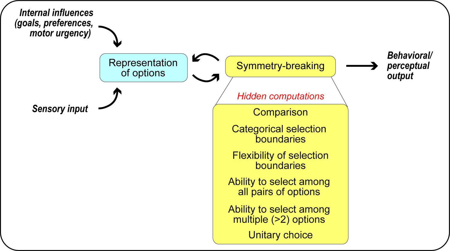
A computational framework for competitive selection based on first principles.
The computational primitives underlying competitive selection are shown as ‘hidden computations’. See also Box 1.
Figure 2
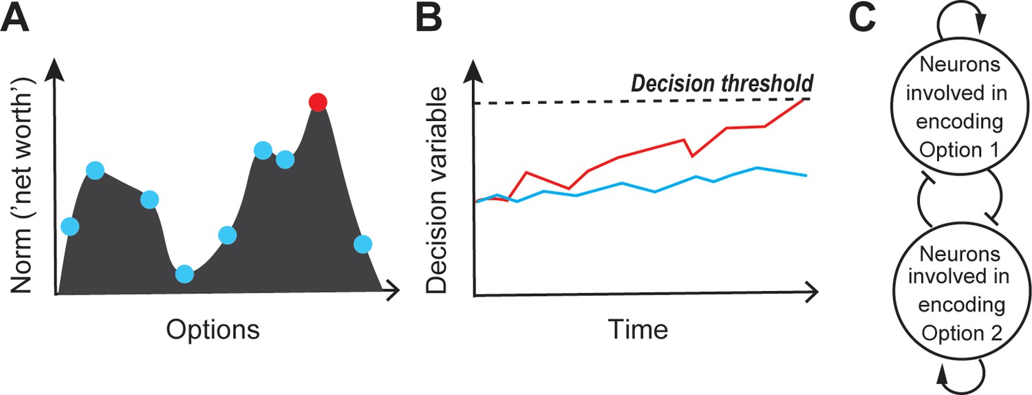
Competitive selection: theory and modeling.
(A) Schematic illustrating the peak-detection formulation of competitive selection. Shown is a representational landscape (depicted here as a continuous ‘hilly’ surface), in which each point corresponds to an option-norm pair. Dots illustrate a few specific option-norm pairs; red dot represents the winning option, i.e., the option corresponding to the highest peak in the landscape. (B) Schematic illustrating the ‘first-to-threshold’ formulation. Shown is the evolution over time of two decision variables, one red and one blue. The winning option is the one (red) that first crosses decision threshold. (C) Modeling. A prominent network architecture involving ‘mutual inhibition’, used in both the winner-take-all (WTA) and accumulation to threshold (A2T) formulations of competitive selection (Roe et al., 2001; Usher and McClelland, 2001; Machens et al., 2005; Wong and Wang, 2006; Mysore and Knudsen, 2012; see text). Arrows with pointed heads denote excitation (recurrent), and those with flat heads denote inhibition.
Figure 3
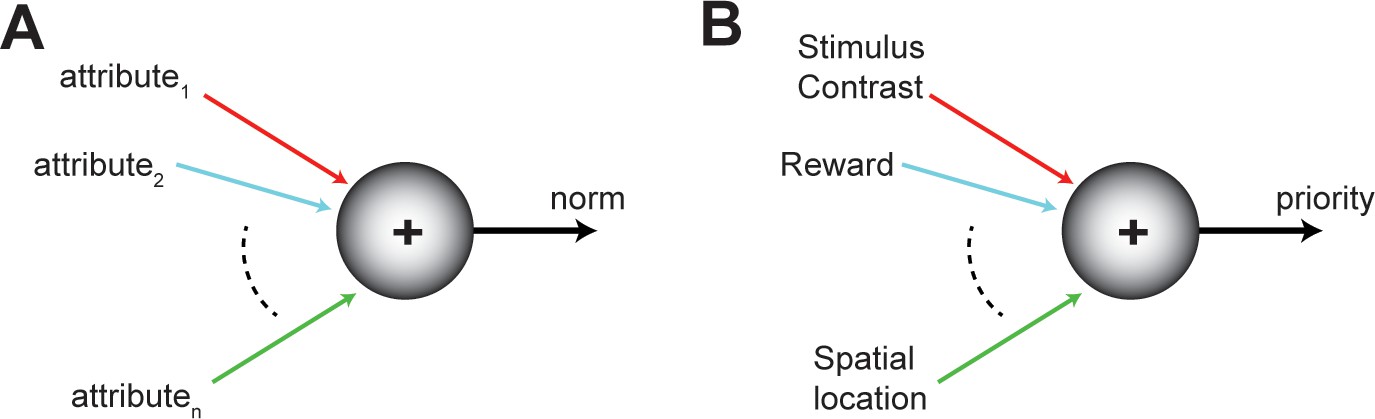
Norm of an option.
(A) Schematic showing the norm of an option as a function of its various attributes (colored axes). The norm of an option encodes its worth to the animal, and can vary from moment to moment. The norm serves as a common frame of reference for comparing among competing options. (B) Illustration of the norm in the context of selective (spatial) attention.
Figure 4
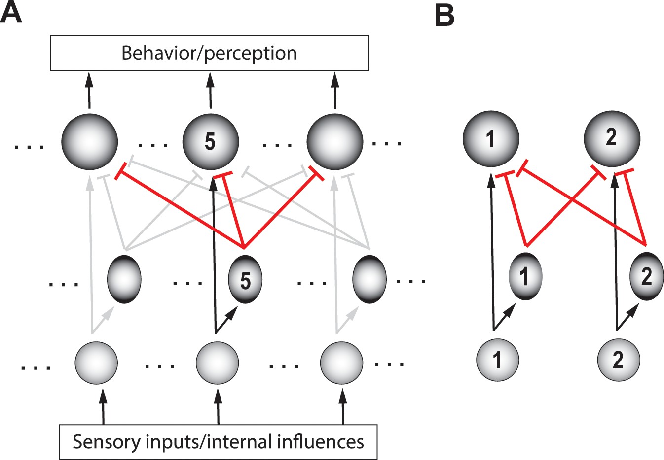
Schematic of a circuit illustrating a motif for comparison.
(A) Rows – layers of neurons; columns – neurons encoding for different options (referred to as ‘channels’); channel #5 neurons are labeled. Bottom layer (small, grey circles) – neurons in the input layer to the selection circuit, which gather information about the various attributes of each option. Middle layer (ovals) – inhibitory neurons. Top layer (large circles) – excitatory neurons that signal the winner. Although each channel is capable of triggering output, only the winning channel will. When only a single option is presented, the corresponding output neuron signals the norm of that option. Arrows with flat heads – inhibitory projections; in black: Excitatory input corresponding to option #5; in red: global feedforward inhibition from option #5 to all options (corresponding to the first computation of comparison); in grey: Excitatory and inhibitory connections corresponding to other options. (B) A two-option version of the circuit in A, redrawn for clarity. Arrows depicting input into the circuit and output from the circuit are not shown here (and in subsequent figures), for simplicity.
Figure 5
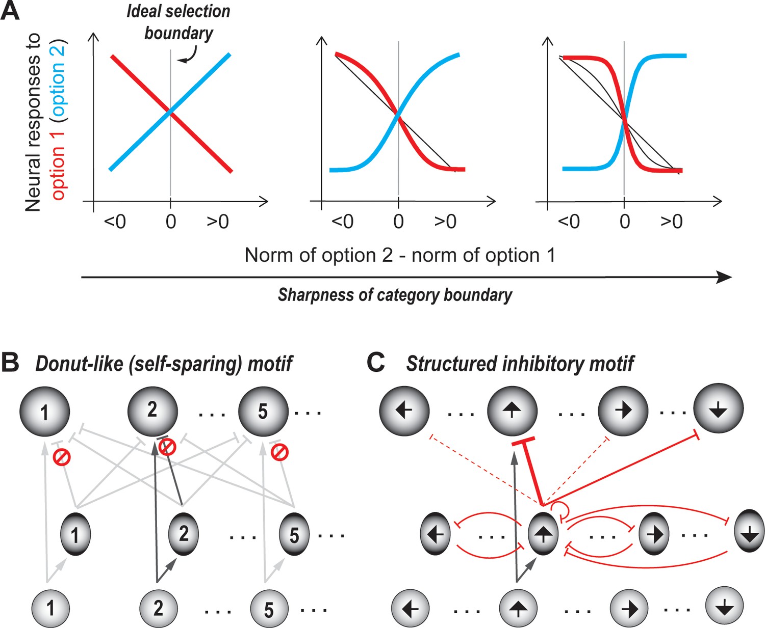
Categorical selection boundary.
(A) Neural response curves showing different degrees of categorical selection in a two option case. X-axis represents the relative norm of the two options, i.e., the difference between the norms of option 2 and option 1. Difference >0: Option two ought to be the winner (option two is stronger than option 1);<0: Option one ought to be the winner (option two is weaker than option 1); Difference = 0/vertical gray line: ideal selection boundary. Y-axes represent the mean responses of neurons that prefer option 1 (red) and option 2 (blue). These can also be thought of as the average probability that option one is going to be signaled by these neurons as the winner. (Only the means are shown for clarity, but in reality, each point on the curve is associated with a distribution of responses.) The leftmost panel illustrates the implementation of an uncertain selection boundary, one that is most vulnerable to sensory ambiguity and neural noise; subsequent panels illustrate the implementation of increasingly categorical boundaries; based on Mahajan and Mysore, 2020. (B) Schematic of selection circuit illustrating the donut-like inhibitory motif for implementing categorical selection boundaries (based on Mahajan and Mysore, 2020). In this circuit, self-inhibition, both feedforward and feedback, is zero (indicated by the red symbol). All other conventions as in Figure 3. (C) Schematic of selection circuit illustrating the structured inhibitory motif for robust-to-noise selection in the context of a circular feature space (such as motion direction (Xue and Liu, 2014). In this circuit, feedforward inhibition to similar feature values (‘self-inhibition’) as well as to opposite feature values is strong (solid red lines), with self-inhibition being the stronger of the two (thicker red line). Feedforward inhibition to all other feature values is very weak (dashed red lines). Feedback inhibition to similar, opposite, and other feature values is of uniform strength (curved red lines).
Figure 6
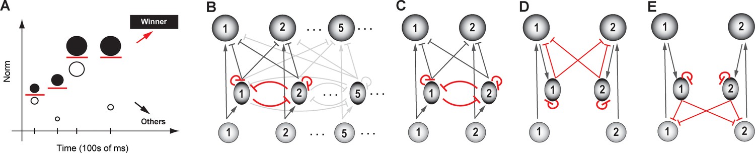
Dynamic flexibility of the selection boundary.
(A) Illustration of the need for a dynamically flexible selection boundary. Tick marks along x-axis: individual trials, or instants at which the set of options (circles parallel to the y-axis) available to the animal changes. For illustrative purposes, we consider only two options being presented in each trial. Filled circle: option with higher norm; open circle: option with lower norm. Red horizontal line: selection boundary; must change dynamically based on the set of options to correctly signal the winner; adapted from Mysore and Knudsen, 2011a. (B) Schematic of selection circuit illustrating motif required for flexibility, namely, feedback inhibition among options (highlighted in red). Feedback is implemented as reciprocal inhibition of inhibition (Mysore and Knudsen, 2012). All other conventions as in Figure 4. (C) A two-option version of the circuit in B, redrawn for clarity. (D, E) Two alternatives to C for implementing feedback inhibition among the options. Both are examples of ‘indirect’ implementation, and involve more synapses and neurons within the feedback loop than the one in B/C; adapted from Mysore and Knudsen, 2012.
Figure 7
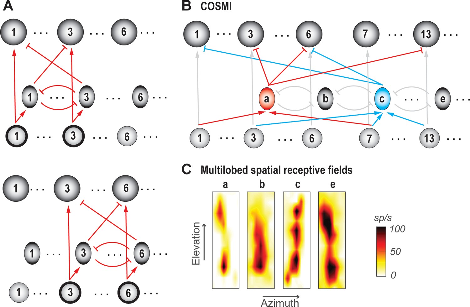
Ability to select among all viable pairs of options.
(A) Schematics illustrating the ‘copy-and paste’ circuit strategy for achieving invariance to option identities. Top panel: Illustrates a scenario in which only options 1 and 3 are available to the animal (indicated by thick outlines around the input neurons 1 and 3 in the bottom layer). All neurons involved in encoding a particular option constitute a neural ‘channel’; shown is channel 3. Bottom panel: Illustrates a different scenario in which only options 3 and 6 are available. Here, selection between channels 3 and 6 is being solved by simply ‘copying-and-pasting’ the circuit module (red connections) used for selection between options 1 and 3. (B) Schematic of selection circuit illustrating the COSMI strategy for achieving invariance to option identities, discovered in the context of selection for spatial attention (Mahajan and Mysore, 2018; Mahajan and Mysore, 2020). COSMI- Combinatorially optimal coding by sparse, multilobe inhibitory neurons (see also Box 3). A group of high-firing inhibitory neurons, fewer in number than the number of spatial locations encoded (or number of channels), encode space densely with spatial receptive fields that have multiple hotspots or lobes. (C) Spatial receptive fields (RFs) of four Imc neurons, three of which are multilobed; neurons a,b,c,e, here, correspond loosely to the ones in B; adapted from Mahajan and Mysore, 2018.
Figure 8
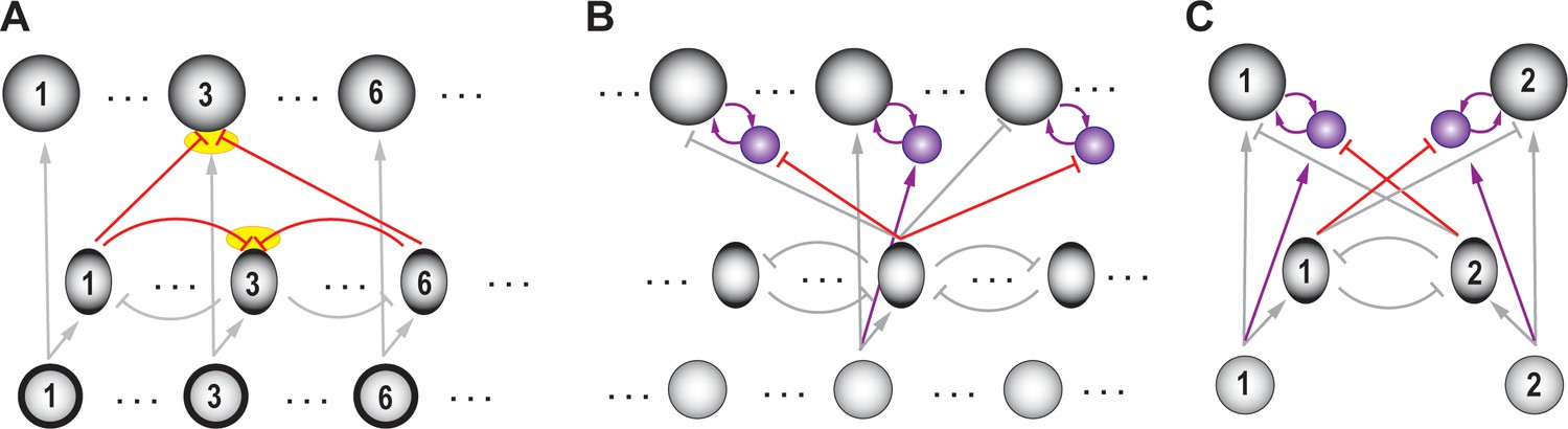
Ability to select among multiple (>2) options, and generation of unitary choice.
(A) Ability to select among more than two options. Schematic of selection circuit illustrating a scenario in which multiple options (here, options 1, 3, and 6) are presented simultaneously. Yellow ovals: Highlights the open question pertaining to the rules by which inhibition (feedforward as well as feedback) from all other options is combined to impact the representation of each option. All other conventions as in previous figures. (B–C) Unitary output generation. (B) Schematic of selection circuit illustrating a potential circuit motif for generating unitary choice (see text). Purple circles: amplifier neurons providing recurrent excitation (purple arrows); they are also recipients of high-gain competitive inhibition in a donut-like pattern (red arrows) (Mahajan and Mysore, 2020). (C) A two-option version of the circuit in B, redrawn for clarity.
Figure 9
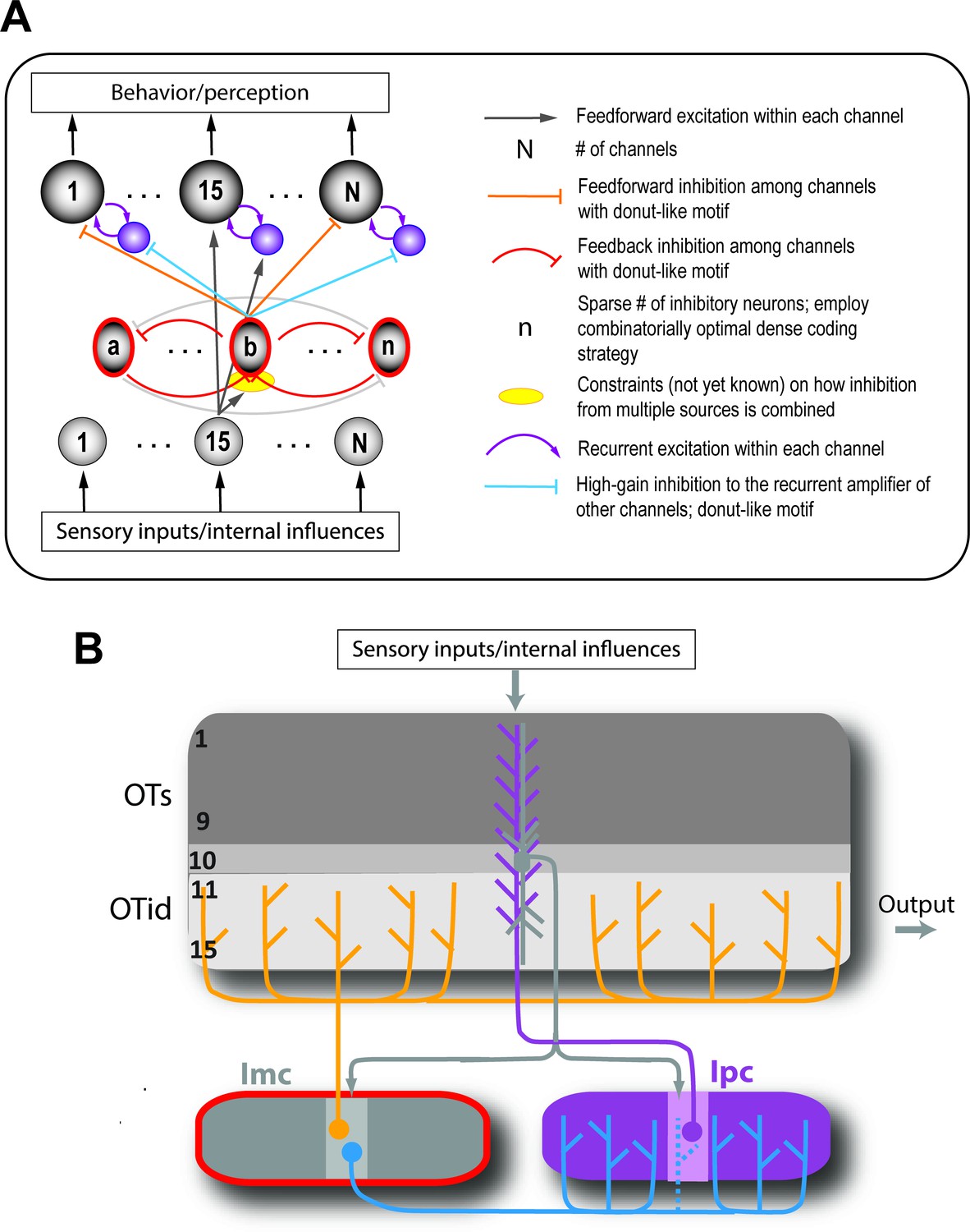
Canonical circuit for competitive selection.
(A) Schematic combining the circuit motifs from Figure 4 through Figure 8. It represents the proposed neural circuit implementation corresponding to the framework for competitive selection (Figure 1). Only connections with respect to channel 15 are highlighted, for visual clarity. (B) The spatial selection circuit in the avian midbrain, thought to be conserved across vertebrates, parallels the proposed circuit. It includes the optic tectum (OT, superior colliculus in mammals), GABAergic isthmi neurons (Imc; grey structure with red outline), and cholinergic isthmi neurons (Ipc; purple structure).
Figure 10
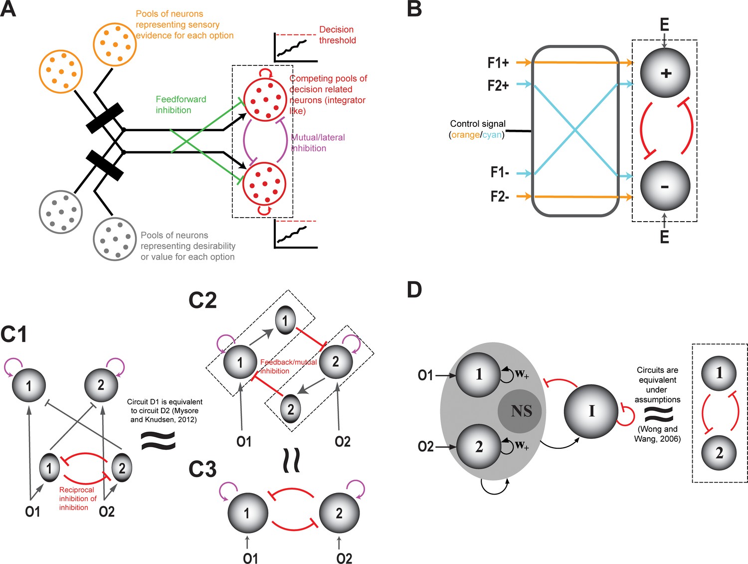
Comparison with prominent models of competitive selection.
In all panels, shaded circles and ovals represent neurons or neural populations; arrows with triangular heads indicate excitatory connections, and with flat heads, inhibitory connections. O1 and O2 represent two options. (A) Schematic of a model of decision-making adapted from Roe et al., 2001, Usher and McClelland, 2001; Usher and McClelland, 2004, Churchland and Ditterich, 2012. (B) Model of decision-making and working memory in a tactile delayed match-to-sample task adapted from Machens et al., 2005. F1 is the first stimulus presented (tactile stimulation), F2 is the stimulus presented after a delay. F1+/F2+ (F1-/F2-) represent neurons that respond with increasing (decreasing) firing rates for increasing tactile stimulation frequency. The (+) and (-) represent pools of decision making neurons which mutually inhibit each other via feedback inhibition. The control signal helps route information from the F+/F- pools of neurons to the decision-making pools. The two states of the control signal are depicted here with two colors – orange and cyan. (C) C1 shows a 2-option version of the competitive selection framework proposed here (and found in several species – see subsection titled ‘Plausibility: Biological…’). C2 shows a circuit equivalent of the model in C1 (Mysore and Knudsen, 2012) which can be reduced to the classic mutual inhibition model. C3 shows the high-level, mutual inhibition model that summarizes all the models discussed in A,B and C; same as Figure 2C. Note that C2 implements a combination of feedback inhibition and donut-like inhibition (Mahajan and Mysore, 2020). (D) A recurrent network model of decision-making and time-integration (Amit and Brunel, 1997; Wang, 2002; Lo and Wang, 2006; Wong and Wang, 2006; Furman and Wang, 2008; Louie et al., 2011; Deco et al., 2013) (Adapted from Wong and Wang, 2006). Under special assumptions of linear input-output functions and gating variables, this model also reduces to the classic mutual inhibition model in C3. I: denotes population of inhibitory neurons; NS: denotes population of neurons nonselective for either input.
Download links
A two-part list of links to download the article, or parts of the article, in various formats.
Downloads (link to download the article as PDF)
Open citations (links to open the citations from this article in various online reference manager services)
Cite this article (links to download the citations from this article in formats compatible with various reference manager tools)
Mechanisms of competitive selection: A canonical neural circuit framework
eLife 9:e51473.
https://doi.org/10.7554/eLife.51473


