Local cortical desynchronization and pupil-linked arousal differentially shape brain states for optimal sensory performance
- University of Lübeck, Germany
Figures
Figure 1
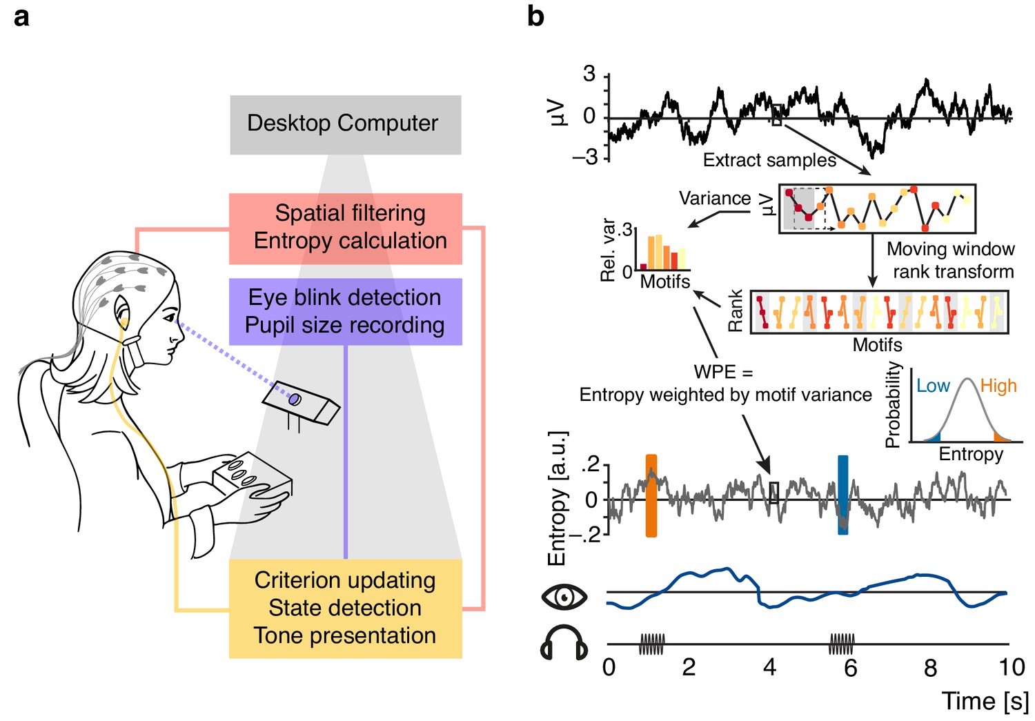
Illustration of the real-time closed-loop setup to track states of desynchronization.
(a) Setup: EEG signal was spatially filtered before entropy calculation. Pupil size was recorded and monitored consistently. Pure tone stimuli were presented via in-ear headphones during states of high or low entropy of the incoming EEG signal. (b) Schematic representation of the real-time algorithm: spatially filtered EEG signal (one virtual channel) was loaded before entropy was calculated using a moving window approach (illustrated for 18 samples in the upper box; 200 samples were used in the real-time algorithm). Voltage values were transformed into rank sequences (‘motifs’) separated by one sample (lower box; Equation 1 in Materials and methods; different colours denote different motifs), and motif occurrence frequencies were weighted by the variance of the original EEG data constituting each occurrence (Equations 3 and 4). Each entropy value was calculated based on the resulting conditional probabilities of 200 samples, before the window was moved 10 samples forward (i.e., effectively down-sampling to 100 Hz). Inset: The resulting entropy time-course was used to build a continuously updated distribution (forgetting window = 30 s). Ten consecutive entropy samples higher than 90% (or lower than 10%) of the currently considered distribution of samples defined states of relatively high and low desynchronization, respectively. Additionally, pupil size was sampled continuously.
Figure 2 with 1 supplement
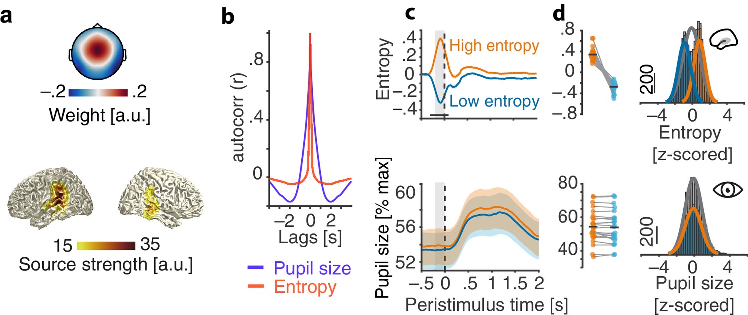
Evaluation of the real-time closed-loop setup for states of local desynchronization and arousal.
(a) Grand average spatial filter weights based on data from an auditory localizer task (top) and grand average source projection of the same data (masked at 70% of maximum; bottom). (b) Autocorrelation functions for EEG entropy (red) and pupil size time courses (blue). Entropy states are most self-similar at ~500 ms (~2 Hz) and pupil states at ~2 s (~0.5 Hz). (c) Grand average time-courses of entropy (upper panel) and pupil diameter (lower panel) for low-entropy (blue) and high-entropy states (orange) ± standard error of the mean (SEM). Subject-wise averages in the pre-stimulus time-window (−200–0 ms, grey boxes) in right panels. Entropy was logit transformed and baseline corrected to the average of the preceding 3 s for illustration. Pupil size was expressed as percentage of each participant’s maximum pupil diameter across all pre-stimulus time-windows. (d) Histograms and fitted distributions of absolute z-scored pre-stimulus entropy (top) and z-scored pupil size (bottom) for low-entropy states (blue), high-entropy states (orange), and both states combined (grey). Note the independence of entropy states and pupil states.
Figure 2—figure supplement 1
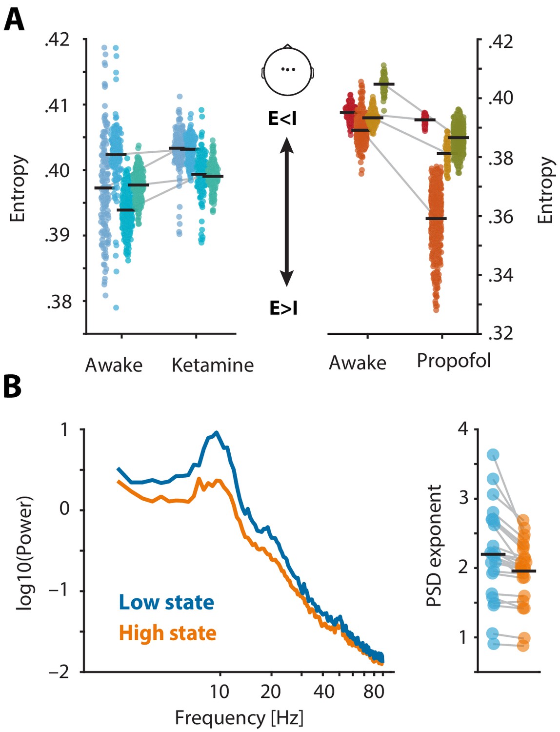
EEG entropy as a marker of E/I balance based on anaesthesia recordings from Sarasso et al. (2015).
Figure 3 with 1 supplement

Contribution of pre-stimulus entropy and pupil size to ongoing auditory cortical EEG activity.
(a) Grand average gamma power across time (40–70 Hz, baselined to the whole trial average, in dB) for low states (left), high states (middle) and the difference of both (right). Entropy states are shown in the upper panel, pupil states in the lower panel. Dashed line represents tone onset, white rectangle outlines the pre-stimulus window of interest. (b) As in (a) but for 0–40 Hz. (c) Mean-centred single subject (dots) and grand average gamma power (black lines) in the pre-stimulus time-window (−0.4–0 s), residualized for baseline entropy and pupil size, shown for five bins of increasing pre-stimulus entropy (left) and pupil size (residualized for entropy baseline and pre-stimulus entropy, middle). Grey line represents average fit, red colours show increasing entropy, blue colours increasing pupil size. Effects of entropy and pupil size are contrasted in the right panel. (d) As in (c) but for low-frequency power (1–8 Hz). Note the different y-axis range between entropy and pupil effects. All binning for illustrational purposes only. ***p<0.0001, **p<0.001.
Figure 3—figure supplement 1

Ongoing activity in the alpha and beta band as a function of EEG entropy and pupil size.
Figure 4 with 2 supplements
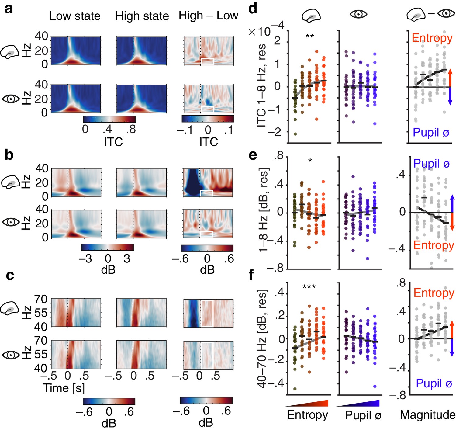
Influence of pre-stimulus entropy and pupil size on tone-related activity.
(a) Grand average ITC (0–40 Hz) across time for low states (left), high states (middle) and the difference of both (right). Entropy states shown in the upper, pupil states in the lower panel. Dashed black lines indicate tone onset, white rectangles the post-stimulus window of interest. (b) As in (a) but for low-frequency power (0–40 Hz, baselined the average of the whole trial). (c) As in (b) but for gamma power (40–70 Hz). (d) Mean centred single subject (dots) and grand average ITC (black lines), residualized for baseline entropy and pupil size, in the post-stimulus time-window (0–.4 s, 1–8 Hz) for five bins of increasing pre-stimulus entropy (left) and pupil size (residualized for entropy baseline and pre-stimulus entropy, middle). Grey line represents average fit, red colours increasing entropy, blue colours increasing pupil size. Effects of entropy and pupil size are contrasted in the right panel. (e) As in (d) but for post-stimulus low-frequency power (0–.4 s, 1–8 Hz). (f) As in (e) but for post-stimulus gamma power (0–.4 s, 40–70 Hz). Again, all binning for illustrational purposes only. ***p<0.0001, **p<0.001, *p<0.05.
Figure 4—figure supplement 1
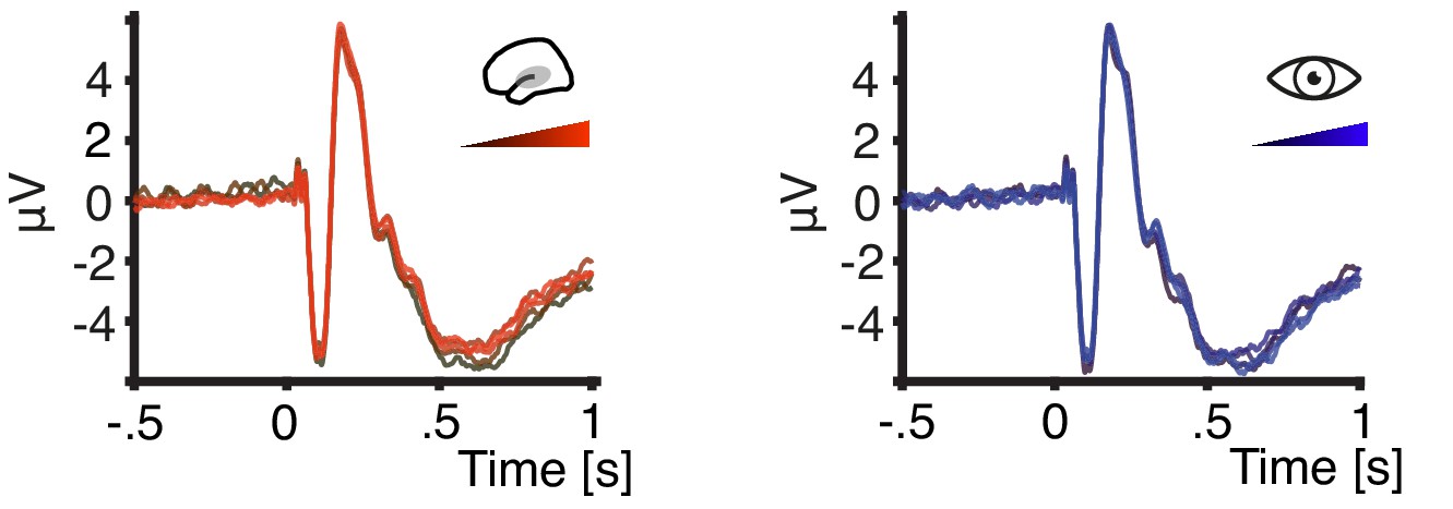
Grand average ERPs for increasing pre-stimulus entropy and pupil size.
Figure 4—figure supplement 2

Tone-related activity in the alpha and beta band as a function of pre-stimulus EEG entropy and pupil size.
Figure 5 with 2 supplements

Effects of pre-stimulus entropy and pre-stimulus pupil size on perceptual performance.
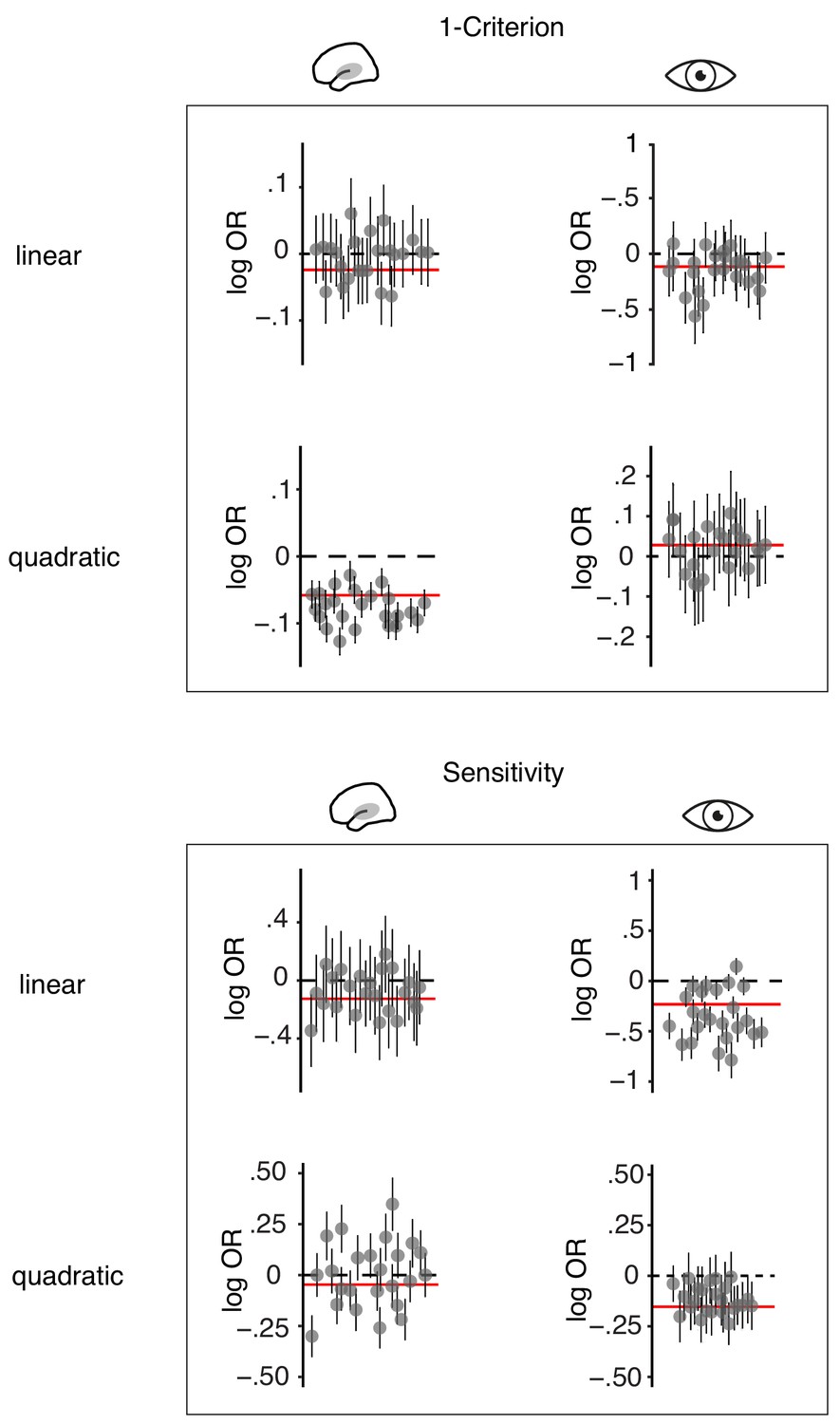
(a) Fixed effects results: probability of judging one tone as ‘high’ as a function of pitch difference from the median (normalized), resulting in grand average psychometric functions for five bins of increasing entropy (red colours) including point estimates ± 1 SEM. Dashed grey lines indicate bias-free response criterion. Insets show 1–criterion (upper) and sensitivity estimates (lower) ±2 SEMs. Bottom left panel shows single subject log odds (log OR) for the quadratic relationship of pre-stimulus entropy and response criterion (±95 % CI), bottom right panel single subject log ORs for the quadratic relationship of pre-stimulus entropy and sensitivity. Participants sorted for log OR, red line marks fixed effect estimate. (b) As in (a) but for five bins of increasing pre-stimulus pupil size. (c) Single subject (dots) and average response speed (black lines) as a function of increasing pre-stimulus entropy (five bins). (d) As in (c) but as a function of pre-stimulus pupil size. Again, all binning for illustration only. *p<.005.
Figure 5—figure supplement 1
Overview of fixed and random effects.
Figure 5—figure supplement 2
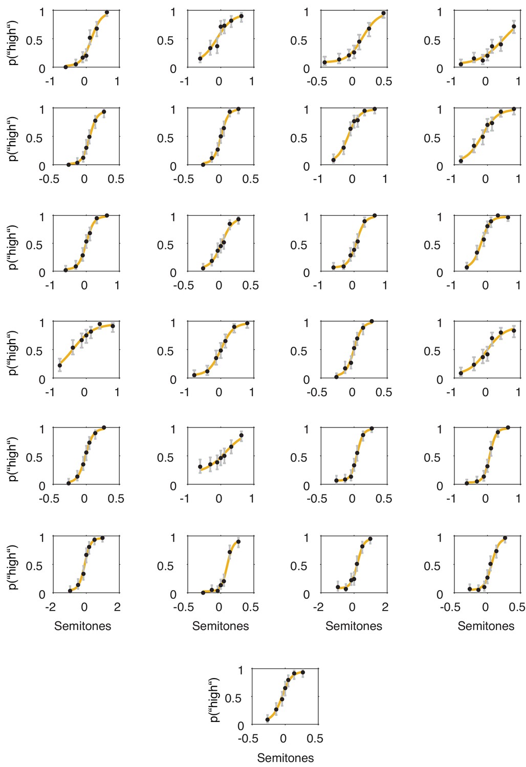
Single participant psychometric functions.
Figure 6 with 1 supplement
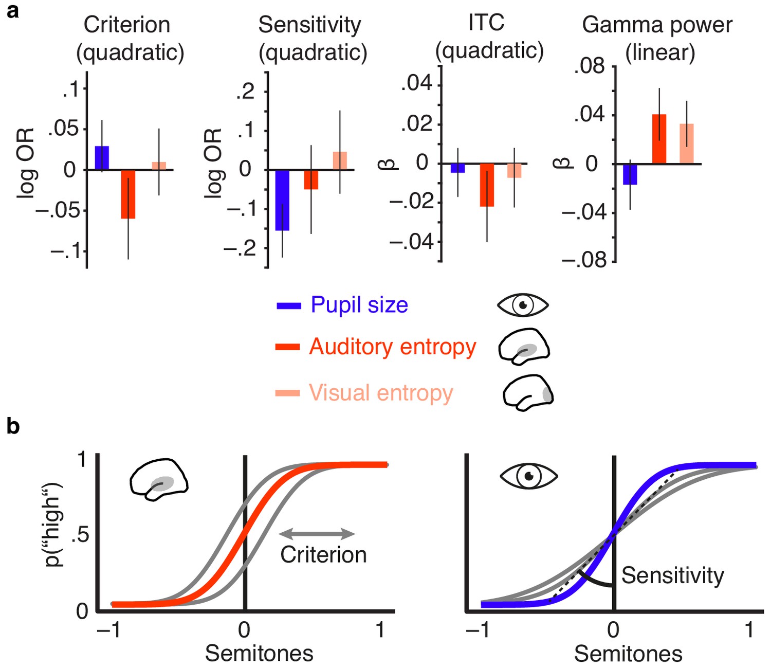
Distinct effects of local desynchronization (i.e., auditory entropy) and global arousal (i.e., pupil size).
(a) Effect sizes (fixed effects, with 95% confidence intervals) for the quadratic relationships of criterion and sensitivity with pupil size (blue), auditory cortex entropy (red) and visual cortex entropy (pale pink). Similarly for the quadratic relationship of pupil size, auditory cortex entropy, and visual cortex entropy with ITC and linear relationships with stimulus-related gamma power. (b) Illustrating the quadratic influence of entropy on response criterion (left panel) and pupil size on sensitivity (right panel) by means of an optimal psychometric function (red vs. blue) and non-optimal ones (grey).
Figure 6—figure supplement 1
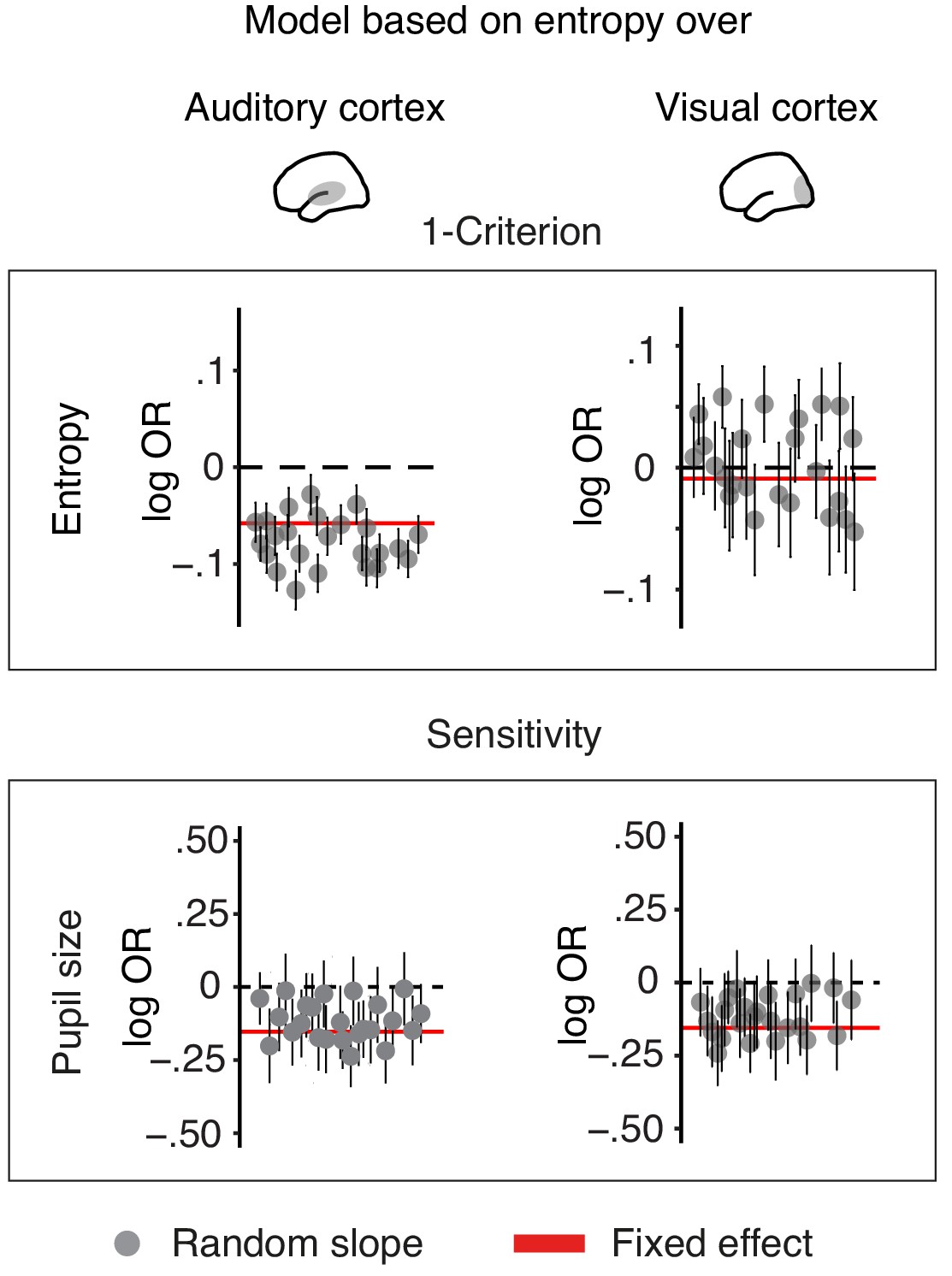
Comparison of results from different brain–behaviour models.
Author response image 1
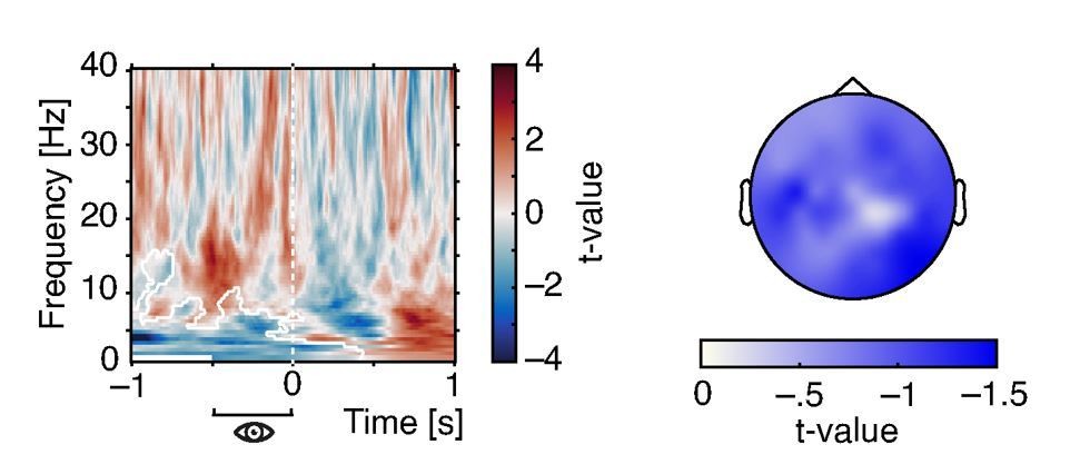
Effects of pre-stimulus pupil size on oscillatory power.
Time-frequency resolved t-values from a cluster test on regression coefficients expressing the relationship between pre-stimulus pupil size (averaged between –.5 and 0 s) oscillatory power (left). Note the negative cluster covering low frequencies (white outlines). T-values averaged over time and frequency points within the significant cluster display a wide-spread topography that peaks over occipito-parietal regions (right).
Additional files
-
Supplementary file 1
Estimates and statistics of the model predicting pre-stimulus low-frequency power.
The table shows model coefficients, standard errors, effect size estimates as well as goodness of fit statistics for the model reported in results and discussion sections.
- https://cdn.elifesciences.org/articles/51501/elife-51501-supp1-v2.docx
-
Supplementary file 2
Estimates and statistics of the model predicting pre-stimulus alpha power.
The table shows model coefficients, standard errors, effect size estimates as well as goodness of fit statistics for the model reported in results and discussion sections.
- https://cdn.elifesciences.org/articles/51501/elife-51501-supp2-v2.docx
-
Supplementary file 3
Estimates and statistics of the model predicting pre-stimulus beta power.
The table shows model coefficients, standard errors, effect size estimates as well as goodness of fit statistics for the model reported in results and discussion sections.
- https://cdn.elifesciences.org/articles/51501/elife-51501-supp3-v2.docx
-
Supplementary file 4
Estimates and statistics of the model predicting pre-stimulus gamma power.
The table shows model coefficients, standard errors, effect size estimates as well as goodness of fit statistics for the model reported in results and discussion sections.
- https://cdn.elifesciences.org/articles/51501/elife-51501-supp4-v2.docx
-
Supplementary file 5
Estimates and statistics of the model predicting post-stimulus low-frequency power.
The table shows model coefficients, standard errors, effect size estimates as well as goodness of fit statistics for the model reported in results and discussion sections.
- https://cdn.elifesciences.org/articles/51501/elife-51501-supp5-v2.docx
-
Supplementary file 6
Estimates and statistics of the model predicting post-stimulus alpha power.
The table shows model coefficients, standard errors, effect size estimates as well as goodness of fit statistics for the model reported in results and discussion sections.
- https://cdn.elifesciences.org/articles/51501/elife-51501-supp6-v2.docx
-
Supplementary file 7
Estimates and statistics of the model predicting post-stimulus beta power.
The table shows model coefficients, standard errors, effect size estimates as well as goodness of fit statistics for the model reported in results and discussion sections.
- https://cdn.elifesciences.org/articles/51501/elife-51501-supp7-v2.docx
-
Supplementary file 8
Estimates and statistics of the model predicting post-stimulus gamma power.
The table shows model coefficients, standard errors, effect size estimates as well as goodness of fit statistics for the model reported in results and discussion sections.
- https://cdn.elifesciences.org/articles/51501/elife-51501-supp8-v2.docx
-
Supplementary file 9
Estimates and statistics of the model predicting post-stimulus low-frequency phase coherence.
The table shows model coefficients, standard errors, effect size estimates as well as goodness of fit statistics for the model reported in results and discussion sections.
- https://cdn.elifesciences.org/articles/51501/elife-51501-supp9-v2.docx
-
Supplementary file 10
Estimates and statistics of the model predicting decisions (high vs. low).
The table shows model coefficients, standard errors, effect size estimates as well as goodness of fit statistics for the model reported in results and discussion sections.
- https://cdn.elifesciences.org/articles/51501/elife-51501-supp10-v2.docx
-
Supplementary file 11
Estimates and statistics of the model predicting decisions based on visual cortex entropy.
The table shows model coefficients, standard errors, effect size estimates as well as goodness of fit statistics for the model reported in results and discussion sections.
- https://cdn.elifesciences.org/articles/51501/elife-51501-supp11-v2.docx
-
Supplementary file 12
Estimates and statistics of the model predicting response speed.
The table shows model coefficients, standard errors, effect size estimates as well as goodness of fit statistics for the model reported in results and discussion sections.
- https://cdn.elifesciences.org/articles/51501/elife-51501-supp12-v2.docx
-
Transparent reporting form
- https://cdn.elifesciences.org/articles/51501/elife-51501-transrepform-v2.pdf
Download links
A two-part list of links to download the article, or parts of the article, in various formats.
Downloads (link to download the article as PDF)
Open citations (links to open the citations from this article in various online reference manager services)
Cite this article (links to download the citations from this article in formats compatible with various reference manager tools)
Local cortical desynchronization and pupil-linked arousal differentially shape brain states for optimal sensory performance
eLife 8:e51501.
https://doi.org/10.7554/eLife.51501


