Gradients in the mammalian cerebellar cortex enable Fourier-like transformation and improve storing capacity
- Leipzig University, Germany
- VU University, Netherlands
- CNRS, Université de Strasbourg, France
Figures
Figure 1 with 3 supplements
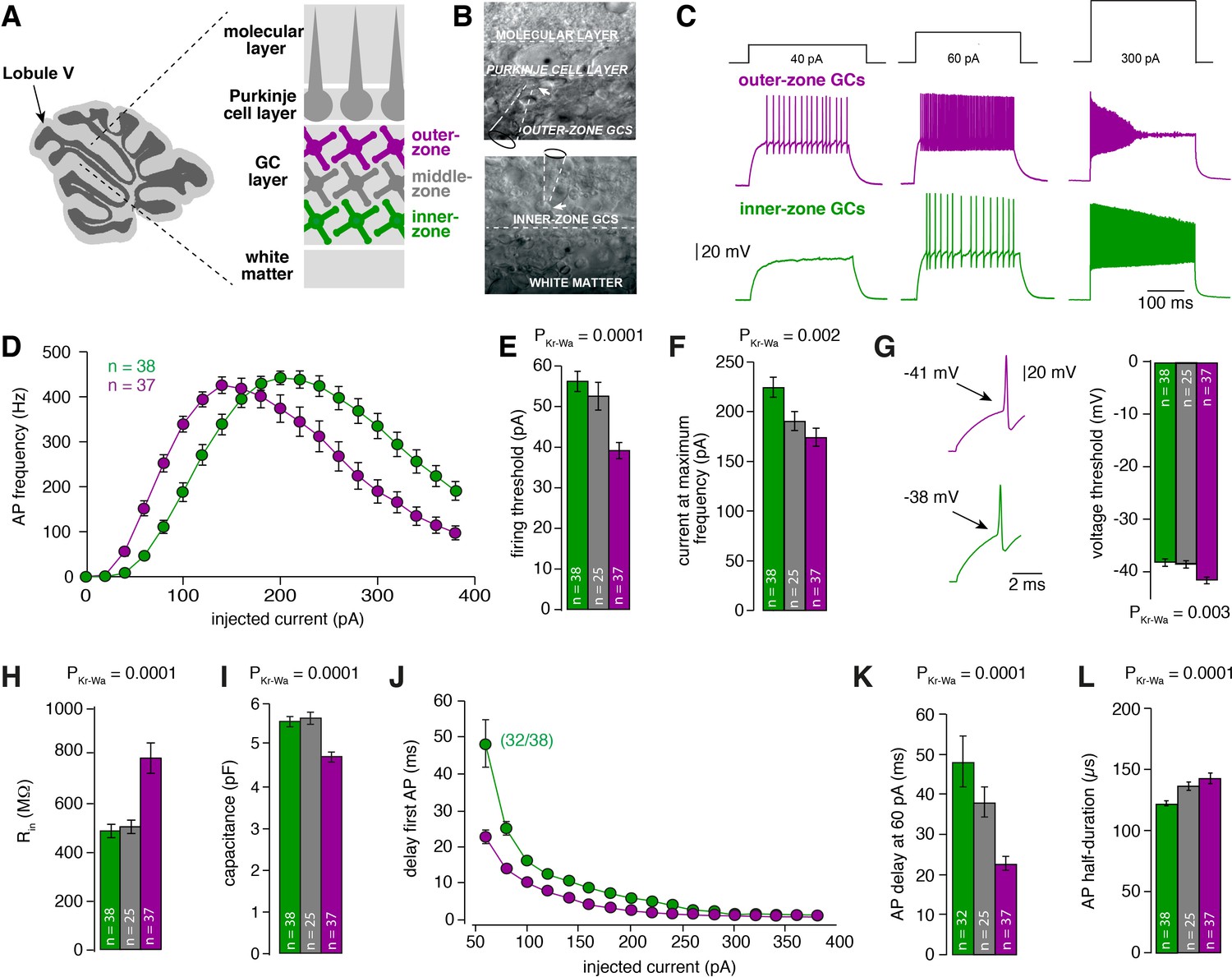
Gradients in the biophysical properties of inner- to outer-zone GCs.
(A) Scheme of a parasagittal slice from the cerebellar cortex where lobule V is indicated by an arrow. Enlargement shows a schematic representation of the white matter, the GC, PC and molecular layer of the cerebellar cortex. Throughout the manuscript, inner-zone GCs (close to the white matter) are depicted in green, the middle-zone GCs in gray, and the outer-zone GC (close to the PCs) in magenta. (B) Example differential-interference-contrast (DIC) microscopic images of acute cerebellar slices during recordings from outer- (top) and an inner-zone GCs (bottom). The pipette is indicated with a dashed line. (C) Example current-clamp recordings from an outer-zone GC (magenta, top) and an inner-zone GC (green, bottom) after injection of increasing currents (40 pA, 60 pA and 300 pA). (D) Average action potential frequency from inner- (green, n = 38) and outer- (magenta, n = 37) zone GCs plotted against the injected current. Note that the maximum frequency is similar but outer-zone GCs achieved the maximum firing rate with a lower current injection (error bars represent SEM). (E) Average current threshold for action potential firing of inner-, middle- and outer-zone GCs (PDunns = 0.0001 for inner- vs outer-zone GCs). All bar graphs represent mean and SEM. (F) Average current needed to elicit maximum firing frequency for inner-, middle- and outer-zone GCs (PDunns = 0.001 for inner- vs outer-zone GCs). (G) Left: example action potentials from an inner- and outer-zone GC with the indicated (arrows) mean voltage-threshold for firing action potentials. Right: Comparison of the average voltage threshold for action potential firing (PDunns = 0.006 for inner- vs outer-zone GCs). (H) Average input resistance of inner-, middle- and outer-zone GCs (PDunns = 0.0001 for inner- vs outer-zone GCs). (I) Average capacitance of inner-, middle- and outer-zone GCs (PDunns = 0.0001 for inner- vs outer-zone GCs). (J) Delay time of the first action potential plotted against injected current. Note that only 32 of 38 inner-zone GCs fired action potentials at a current injection of 60 pA. (K) Delay of the first action potential of inner-, middle- and outer-zone GCs at a current injection of 60 pA (PDunns = 0.0001 for inner- vs outer-zone GCs). (L) Average action potential half-duration of inner-, middle- and outer-zone GCs (PDunns = 0.0001 for inner- vs outer-zone GCs).
Figure 1—figure supplement 1
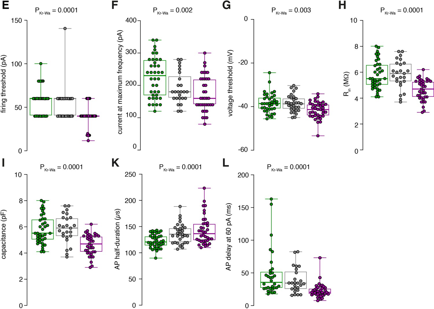
Raw data of the bar graphs from Figure 1.
Figure 1—figure supplement 2
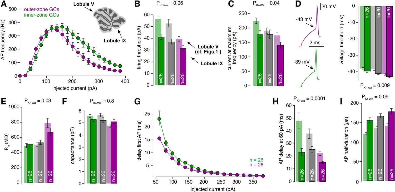
Gradients in the biophysical properties of GCs and PFs are preserved throughout the cerebellar cortex.
(A) Average action potential frequency from inner (green) and outer-zone GCs (magenta) plotted against the injected current. Inset: An image of a cerebellar slice indicating lobule V and lobule IX by arrows. (B) Bar graphs represent the firing threshold of GCs from inner (dark-green), middle (dark-gray) and outer-zone (dark-magenta). The light-colored bar graphs in the background are the data from lobule V shown in Figure 1. Firing threshold is higher in inner- compared to outer-zone GCs from lobule IX, and with the same current injection, GCs from lobule IX fire action potentials faster compared to lobule V. The numbers of recorded GCs for lobule IX (n) are indicated (PDunns = 0.06 for inner- vs outer-zone GCs). (C) Average current needed to elicit the maximum number of action potentials for of inner- (green), middle- (gray) and outer-zone GCs (magenta) (PDunns = 0.06 for inner- vs outer-zone GCs). (D) Left: example action potentials from an inner- and outer-zone GC with the indicated (arrows) mean voltage threshold for firing action potentials. Right: Average voltage threshold to elicit action potentials in inner-, middle- and outer-zone GCs from lobule IX compared with data from lobule V. Voltage threshold for outer-zone GCs is lower compared to inner-zone GCs from lobule IX (PDunns = 0.009 for inner- vs outer-zone GCs). (E) Input resistance of GCs from outer-zone of lobule IV is higher compared to inner- and middle-zone GCs but there is no difference between the input resistance of GCs from lobule V and IX (PDunns = 0.03 for inner- vs outer-zone GCs). (F) Average capacitance of inner-, middle- and outer-zone GCs. In contrary to lobule V, there is no difference in the capacitance of GC from inner-, middle, or outer-zone (PDunns = 0.8 for inner- vs outer-zone GCs). (G) Delay of the first action potential plotted against the injected current. (H) Delay of the first action potential after a current injection of 60 pA from inner-, middle- and outer-zone GCs from lobule IX compared to lobule V (PDunns = 0.01 for inner- vs outer-zone GCs). (I) The action potential half-duration of inner-zone (dark-green) GCs from lobule IX is shorter compared to middle (dark-gray)- and outer-zone (dark-magenta) GCs (PDunns = 0.09 for inner- vs outer-zone GCs). Compared to lobule V (light-colored bar graphs), the GCs from lobule IX showed a broader action potential half-width.
Figure 1—figure supplement 3
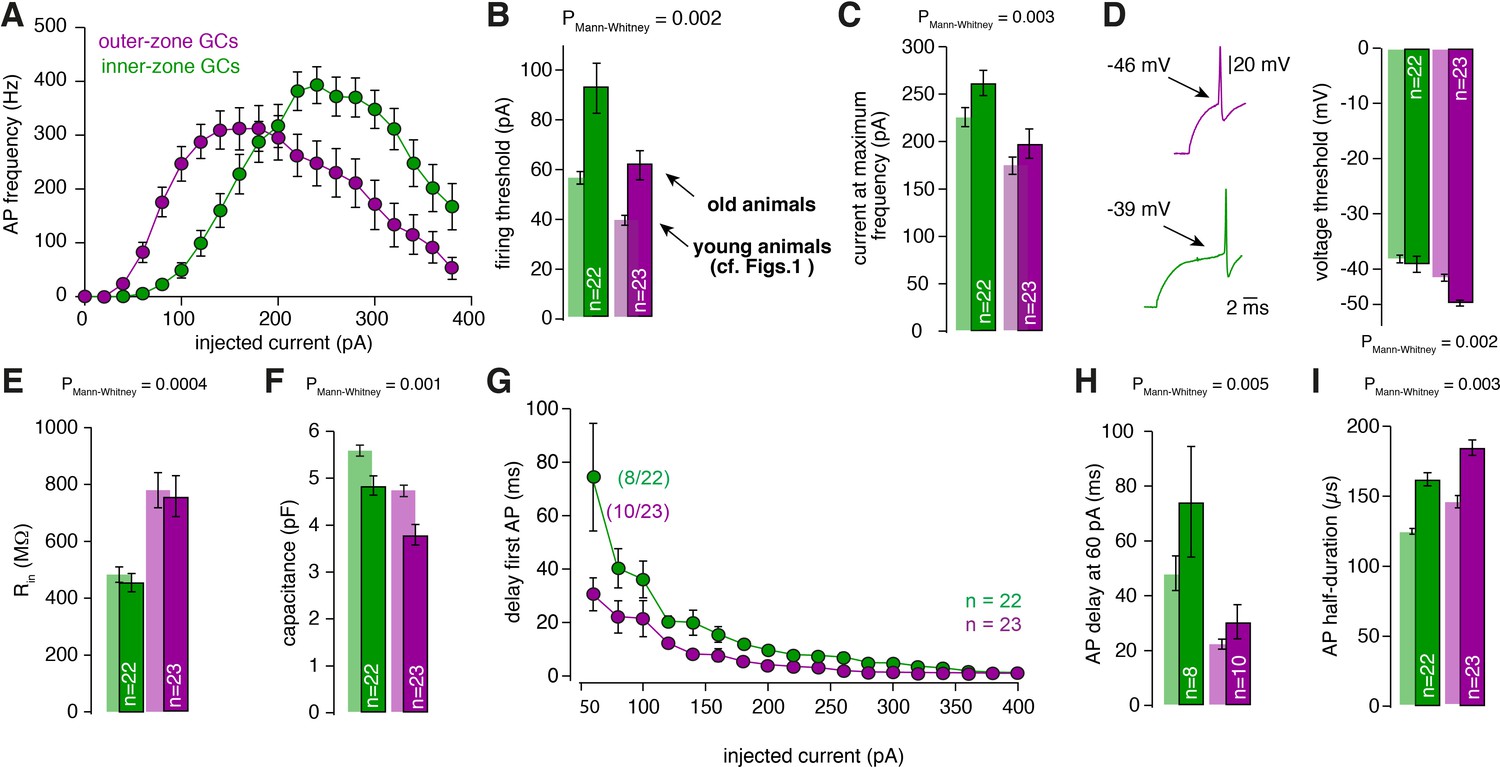
Gradients in the biophysical properties of GCs and PFs are also found in 3-month-old animals.
(A) Average action potential frequency from inner (green) and outer (magenta) zone GCs plotted against the injected current for 3-month-old animals. For all these measurements GCs from lobule V were used. (B) Bar graphs represent the firing threshold of GCs from inner (dark-green) and outer-zone (dark-magenta). The light-colored bar graphs in the background are the data from lobule V in young (21–30 days-old) animals shown in Figure 1. Firing threshold is higher in inner- compared with outer-zone GCs from old animals. (C) Average current needed to elicit the maximum number of action potentials for of inner- (green) and outer-zone GCs (magenta). (D) Left: example action potentials from an inner- and outer-zone GC with the indicated (arrows) mean voltage-threshold for firing action potentials. Right: Average voltage threshold to elicit action potentials in inner and outer-zone GCs from old animals compared with data from young animals. (E) Input resistance of GCs from outer-zone is higher compared to inner-zone GCs. But there is no difference between the input resistance of GCs from young and old animals. (F) Average capacitance of inner- and outer-zone GCs. In agreement with the data from the young animals, inner-zone GCs have a higher capacitance compered to outer-zone GCs. (G) Delay of the first action potential plotted against the injected current. Since the mean current threshold is higher compared to young animals only 8 out of 22 GCs from inner- and 10 out of 23 GCs from outer-zone already fired action potentials at a current injection of 60 pA. (H) Delay of the first action potential after a current injection of 60 pA from inner-, middle- and outer-zone GCs from old animals compared to young animals. (I) The action potential half-duration of inner-zone (dark-green) GCs from old animals is shorter compared with outer-zone (dark-magenta) GCs.
Figure 2 with 2 supplements
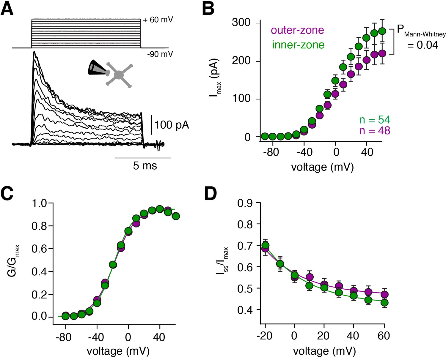
Voltage-gated potassium currents are larger at inner-zone GCs.
(A) Example potassium currents from outside-out patches of cerebellar GCs evoked by voltage steps from −90 to +60 mV in 10 mV increments with a duration of 10 ms. All recordings were made in the presence of 1 µM TTX and 150 µM CdCl2 to block voltage-gated sodium and calcium channels, respectively. (B) Average peak potassium current (Imax) plotted versus step potential of inner (green) and outer-zone (magenta) GCs. Significance level was tested with a Mann-Whitney U Test for the value at +60 mV and the p value is indicated in the figure. (C) Average normalized peak potassium conductance (G/Gmax) versus step potential of inner (green) and outer-zone (magenta) GCs. (D) Average steady-state current (Iss, mean current of the last 2 ms of the 10 ms depolarization) normalized to the peak current (Imax) versus step potential of inner (green) and outer-zone GCs (magenta).
Figure 2—figure supplement 1
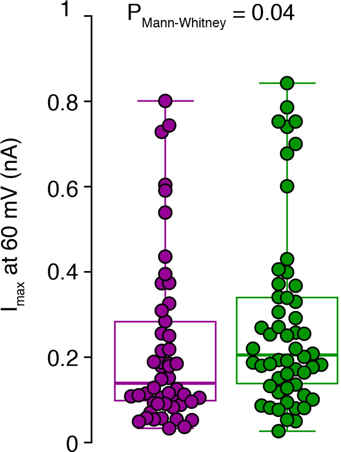
Raw data of the amplitude of potassium currents at 60 pA current injection.
Peak amplitudes of single-cell potassium currents from inner-(green) and outer-zone CGs (magenta) after 60 pA current injection are shown together with box plots (median and interquartile range with whiskers).
Figure 2—figure supplement 2
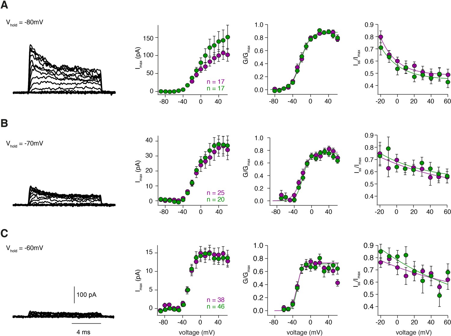
Steady-state activation and inactivation are similar for inner and outer GCs.
(A – C) left: Example potassium currents from outside-out patches of cerebellar GCs evoked by voltage steps from −90 to +60 mV in 10 mV increments with a duration of 10 ms. The intersweep holding potential varied between −80 mV (A), −70 mV (B) and −60 mV (C). Panels show the corresponding current-voltage relationship (first panel) of inner- (green) and outer-zone GCs (magenta), the normalized conductance (second panel) and the normalized inactivation behavior (third panel). The number of measured cells is indicated in the figure.
Figure 3 with 2 supplements

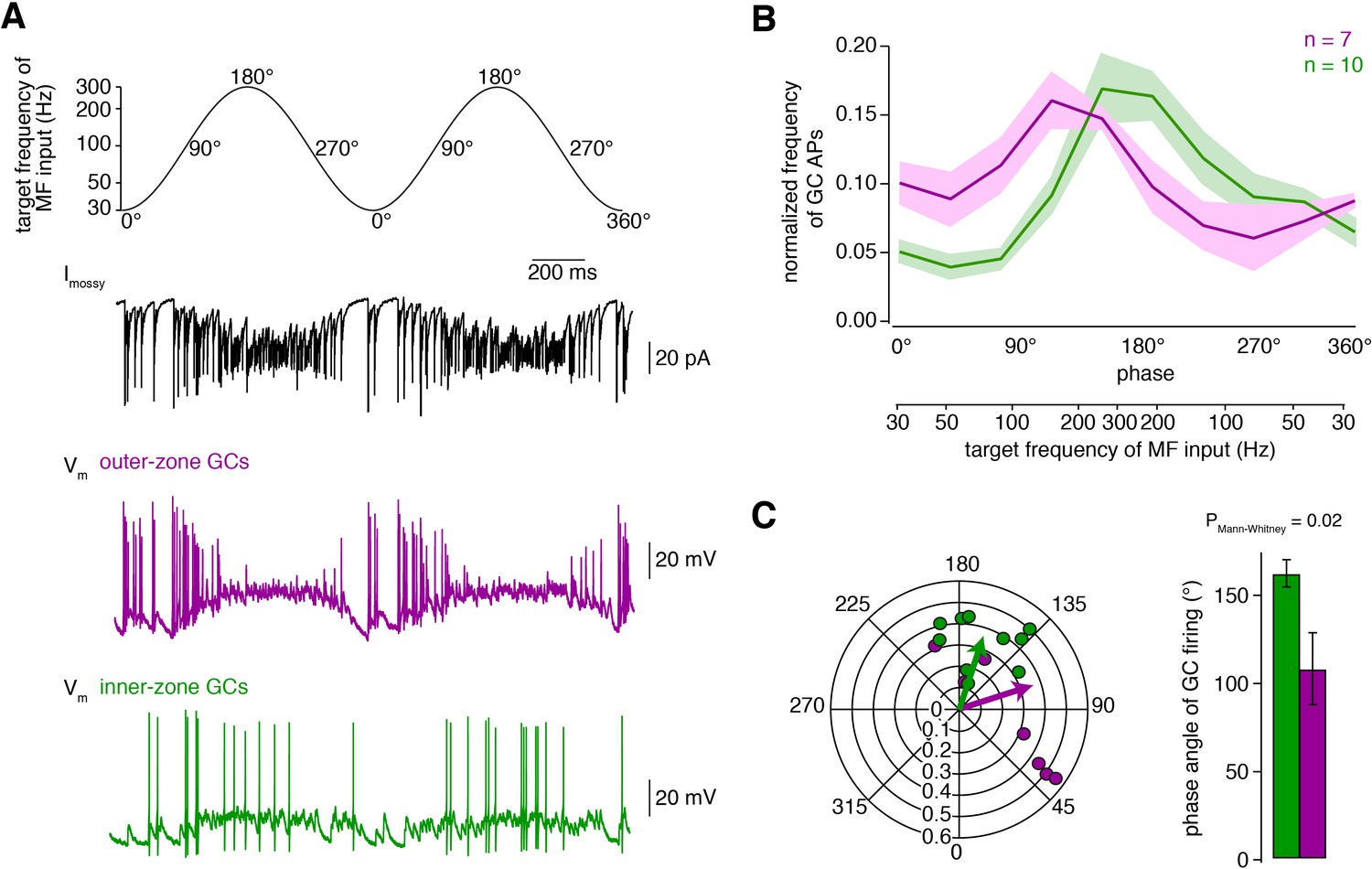
MF inputs are differentially processed by inner- and outer-zone GCs.
(A) Schematic representation of the Dynamic Clamp system. (B) Illustration of MF conductance (Gmossy), GC membrane potential (Vm), and MF current (Imossy) for the Dynamic Clamp technique. Note the prediction of a negative current during an action potential as apparent in the experimental traces in panel C. (C) Example Dynamic Clamp recordings of inner- (green) and outer-zone (magenta) GCs at different holding potentials (−90 mV left; −80 mV middle and −70 mV right) at a stimulation frequency of 100 Hz. Upper traces represent poisson-distributed MF currents. Lower traces show the measured corresponding membrane potential with EPSPs and action potentials. (D) Average firing frequency of inner- and outer-zone GCs during MF- like inputs at different frequencies and at the indicated holding potentials.
Figure 3—figure supplement 1
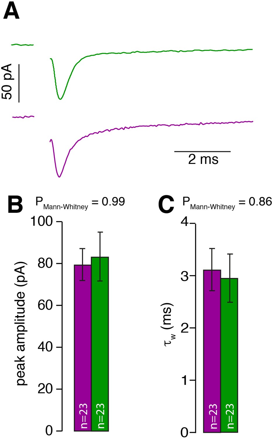
MF input is similar for inner- and outer-zone GCs.
(A) Examples of single EPSCs measured from inner- (green) and outer-zone GCs (magenta) after 1 Hz stimulation of MF axons. Stimulation artifacts were removed. (B) Average amplitude of EPSCs from inner- (green) and outer-zone GCs. (C) Weighted decay time (Equation 4) of EPSCs from inner- (green) and outer-zone GCs (magenta).
Figure 3—figure supplement 2
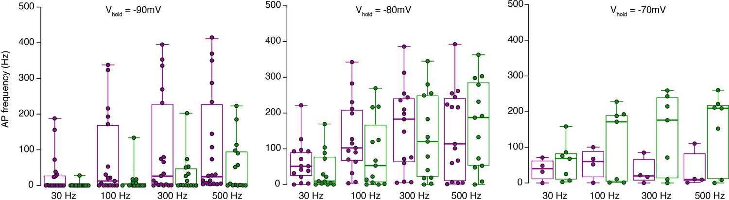
Raw data of the bar graphs from Figure 3. Same data as in Figure 3D, but shown as box plots (median and interquartile range with whiskers) superimposed with single data points.
The same color code as in Figure 3 is used for inner- (green) and outer-zone (magenta) GCs.
Figure 4 with 1 supplement
Fourier-like transformation of MF input frequency.
(A) Target frequency of the Dynamic Clamp MF-like inputs during two cycles. The frequencies varied sinusoidally on a logarithmic scale between 30 to 300 Hz and the cycle duration was 1 s (Equation 2). The degree values denote the phase angle. Black: example trace of poisson-distributed MF-like inputs. Magenta and green: example membrane potential during Dynamic Clamp experiments of an outer- and an inner-zone GC, respectively, at a holding potential of approximately −70 mV. (B) Average normalized frequency of action potentials (APs) fired by inner- and outer-zone GCs (green and magenta, respectively) versus the phase angle and the target MF-like frequency within one cycle (for each cell, the integral of the spike histogram was normalized to 1; see Figure 4—figure supplement 1 for absolute frequency). The light green and magenta areas represent the SEM. (C) Polar plot of phase angle and vector strength of the preferred firing frequency according to Equation 3 from inner- (green) and outer-zone (magenta) GCs (dots: single cells; arrows: average). Bar graph of the average phase angle at which inner- and outer-zone GCs preferentially fired action potentials.
Figure 4—figure supplement 1
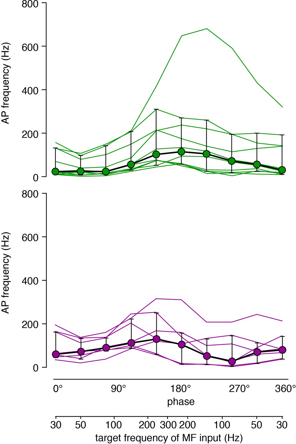
Raw data of the traces shown in Figure 4B.
Data of Figure 4B are shown as single cell data (each cell is one line) superimposed with the median (circles) and interquartile range (error bars). Upper graph: inner-zone GCs in green, lower graph: outer-zone GCs in magenta.
Figure 5

The position of PFs is correlated with the position of GC somata.
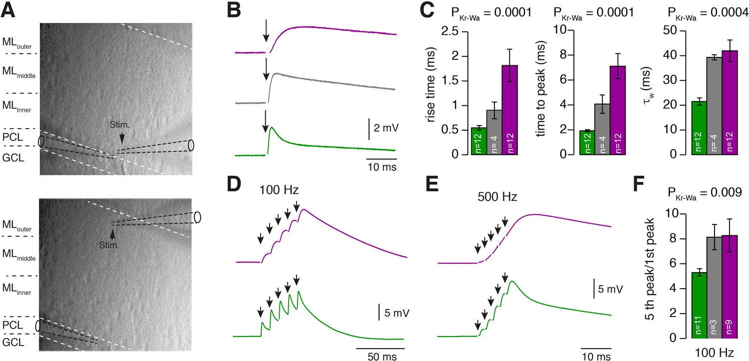
(A) Example of GCs labeled with DiI 24 hr post injection. Numerous GCs from inner-, middle-, and outer-zone were labeled. (B) Example of traced axons from different GCs from the outer zone. The axon was traced (red) from the cell soma to the bifurcation site in the molecular layer. Stained cell bodies of GCs are also visible (white). ML: molecular layer; PCL: Purkinje cell layer; GCL: granule cell layer. (C) The distance between labeled GCs and the PC layer strongly correlated with the distance between the axon bifurcation and the PC layer (Pearson’s correlation coefficient R = –0.86; p<0.001). Solid black line depicts the linear interpolation and the gray lines represent SEM of the fit. The number of GCs (n) is indicated. (D) Position of the GC somata within the GC layer of each traced cell linked to the position of the bifurcation site in the molecular layer. The distances were normalized to the height of the corresponding layers.
Figure 6 with 2 supplements
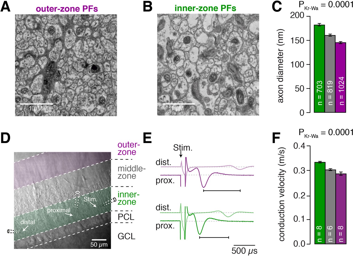
Inner-zone PFs have larger diameter and higher action potential conduction velocity.
(A) Electron microscopic image of the outer (A) and inner zone (B) of sagittal sections through the molecular layer. (C) Summary of axon diameters in the inner- (green), middle- (gray), and outer-zone (magenta) of the molecular layer (PDunns = 0.0001 for inner- vs outer-zone GCs). (D) DIC image of the molecular layer superimposed with a schematic illustration of the experimental setup to measure compound action potentials from PFs. Compound action potentials were evoked by a stimulus electrode (right) and recorded by a proximal and distal recording electrode (middle, left). (E) Example traces used to determine the conduction velocity of inner- and outer-zone PFs. The time difference between the compound action potential arriving at the proximal electrode (solid traces) and the distal electrode (light traces) was used to determine the velocity. The time was shorter for inner-zone PFs (green) compared with outer-zone PFs (magenta). (F) Summary of conduction velocity in inner-, middle- and outer-zones (PDunns = 0.0007 for inner- vs outer-zone GCs).
Figure 6—figure supplement 1
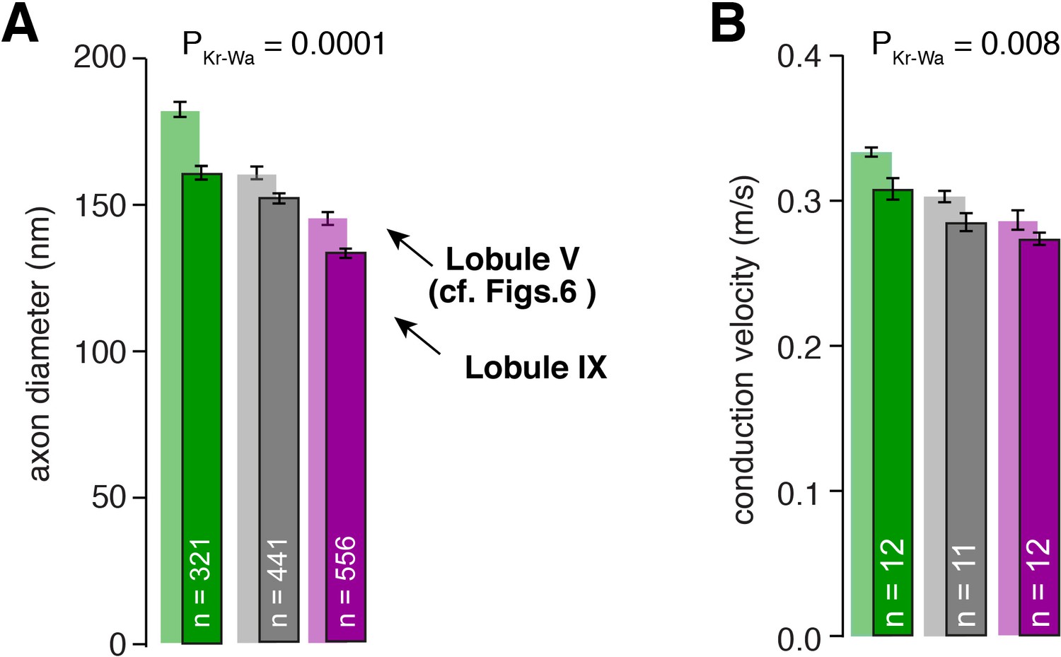
Differences in axon diameter and conduction velocity are also found in lobule IX.
(A) Summary of axon diameters in the inner- (green), middle- (gray), and outer-zone (magenta) of the molecular layer (PDunns = 0.0001 for inner- vs outer-zone GCs). The light-colored bar graphs in the background are the data from lobule V shown in Figure 6. (B) Summary of conduction velocity in the inner-, middle- and outer-zone of of the molecular layer of lobule IX (PDunns = 0.007 for inner- vs outer-zone).
Figure 6—figure supplement 2
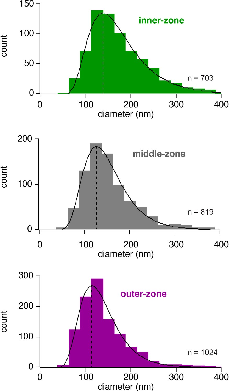
Histogram of the axon diameters.
Histograms of the diameter of inner-, middle- and outer-zone axons in the molecular layer. Data were fit with a skewed Gaussian function: , where a is the amplitude, d the diameter, and d0 the diameter at the peak. ds and b represent parameters related to the width and the skewness, respectively. The peak is indicated by a vertical line.
Figure 7 with 1 supplement
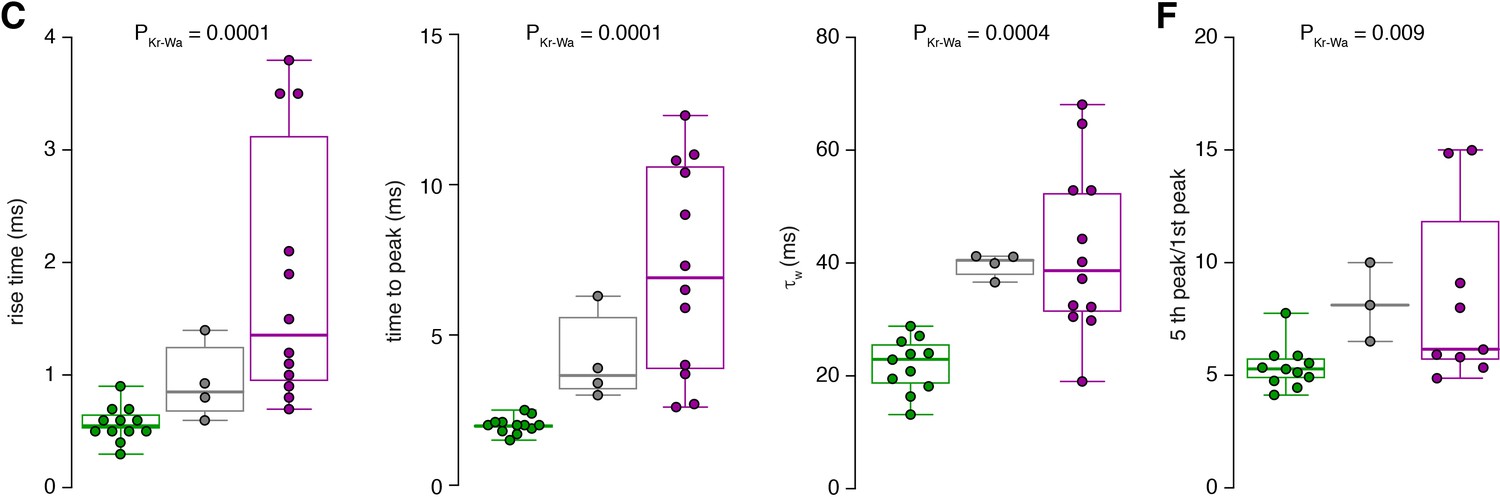
PCs differentially process inner-, middle-, and outer-zone PF inputs.
(A) DIC image of the molecular layer superimposed with a schematic illustration of PC recordings while stimulating inner- (top) and outer-zone PFs (bottom). Shown are the GC layer (GCL), PC layer (PCL) and molecular layer (ML). (B) EPSPs measured at the PC soma after stimulation (1 Hz) of inner- (green), middle- (gray), and outer-zone PFs (magenta). (C) Average 20% to 80% rise time, time to peak and weighted decay time-constant of PC EPSPs after stimulation of inner- (green; n = 12), middle- (gray; n = 4) and outer-zone PFs (magenta; n = 12) as shown in B (PDunns = 0.0001; PDunns = 0.0001; PDunns = 0.0009 for inner- vs outer-zone GCs, respectively). Note, one cell out of 12 had a monoexponentiell decay. (D-E) Example traces of EPSPs from a PC after five impulses to inner- (green) and outer-zone PFs (magenta) at 100 Hz (D) and 500 Hz (E). (F) Average paired-pulse ratio measured in PCs after five 100 Hz stimuli at inner- (green; n = 11), middle- (gray, n = 3) and outer- zone PFs (magenta, n = 8; PDunns = 0.04 for inner- vs outer-zone GCs).
Figure 7—figure supplement 1
Raw data of the bar graphs from Figure 7.
The data from panels of Figure 7 with bar graphs are shown as box plots (median and interquartile range with whiskers indicating the entire range) superimposed with the single data points. The same color code as in Figure 7 is used for inner- (green), middle- (gray) and outer-zone (magenta) GCs, respectively.
Figure 8 with 1 supplement
The observed neuronal gradients increase storing capacity and improve temporal precision of PC spiking.
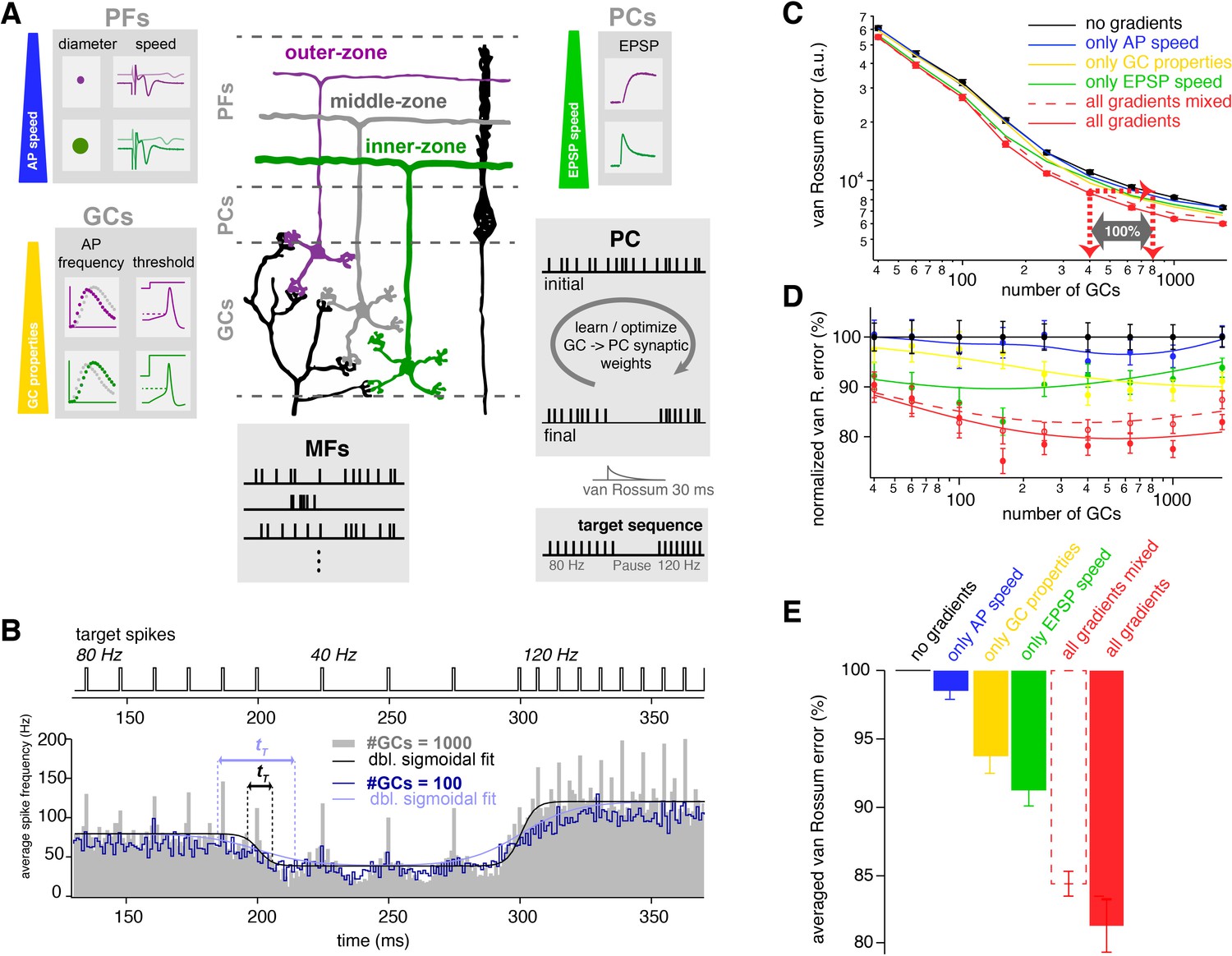
(A) Schematic illustration of the network model of the cerebellar cortex as explained in the main text. (B) Average spiking histogram for models consisting of 100 and 1000 GCs, superimposed with double sigmoidal fits constrained to 80, 40 and 120 Hz. The target spiking sequence is indicated above. tT indicates the transition time of the sigmoidal fit for the respective number of GCs. (C) Double logarithmic plot of the average minimal van Rossum error plotted against the number of GCs for models with no gradients (black), with only gradually varied PF conduction velocity (blue), GC parameters (yellow), )and EPSP kinetics (green), and with all gradients (red). Furthermore, all parameters were gradually varied but the connectivity between GC, PF and EPSPs was random (all gradients mixed; dashed red). Red dashed lines with arrows indicate the number of GCs needed to obtain the same van Rossum error with all gradients compared to no gradients. With no gradients, twice as many GCs are needed to obtain the same van Rossum error. (D) Average van Rossum error as shown in panel C but normalized to values obtaned from the model without gradients, superimposed with a smoothing spline interpolation. (E) Average of the relative differences shown in panel D.
Figure 8—figure supplement 1
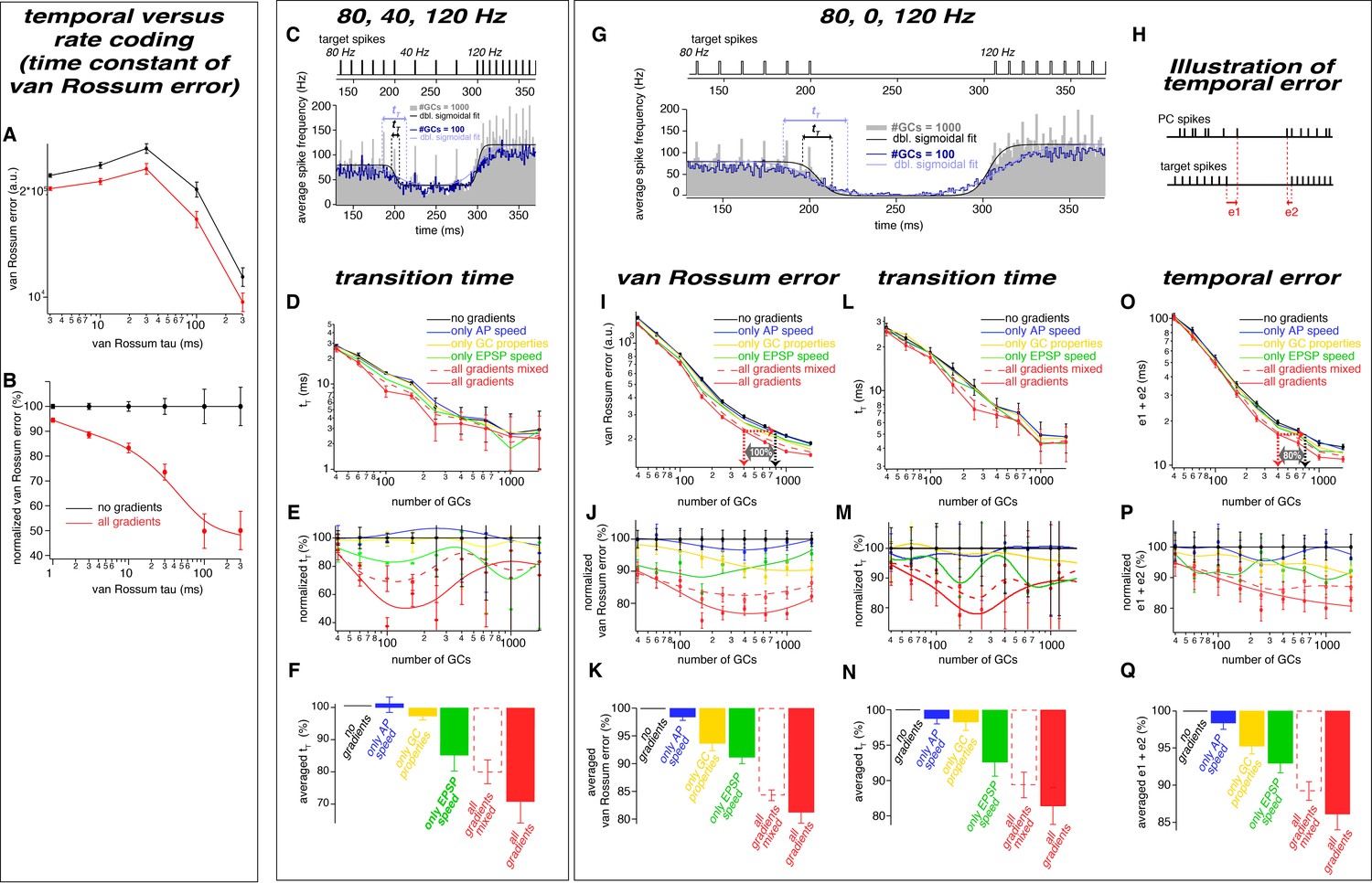
The observed neuronal gradients reduce the temporal error and improve rate coding of PC spikes.
(A) Double logarithmic plot of the van Rossum error of models with 300 GCs without (black) and with all gradients (red) plotted versus the time constant of the van Rossum kernel ranging from 2 to 300 ms. (B) Data as in panel A normalized to the model without gradients. (C) Average spiking histogram for models consisting of 100 and 1000 GCs, superimposed with double sigmoidal fits constrained to 80, 40 and 120 Hz. The target spiking sequence is indicated above. The data is reproduced from Fig. 8B for direct comparison with panel G. (D) Double logarithmic plot of the transition time (tT) of the double exponential fits as illustrated in panel C. To minimize the impact of outliers caused by unstable conversion of double exponential fits, the data presented as median and the error bars represent 95% confidence intervals. (E) Transition time (tT) as shown in panel D but normalized to the value of the model without gradients, superimposed with a smoothing spline interpolation. (F) Average of the relative differences shown in panel E. (G) Average spiking histogram for models consisting of 100 and 1000 GCs, superimposed with double sigmoidal fits constrained to 80, 0 and 120 Hz. The target spiking sequence with 80, 0, and 120 Hz is indicated above. (H) Illustration of the temporal error (e1 and e2) of the spikes defining the beginning and the end of the pause. (I-Q) Analyses for the 80, 0, 120 Hz target sequence including the van Rossum error (I-K), the transition time (tT) (L-N) and the temporal error (O-Q).
Figure 9
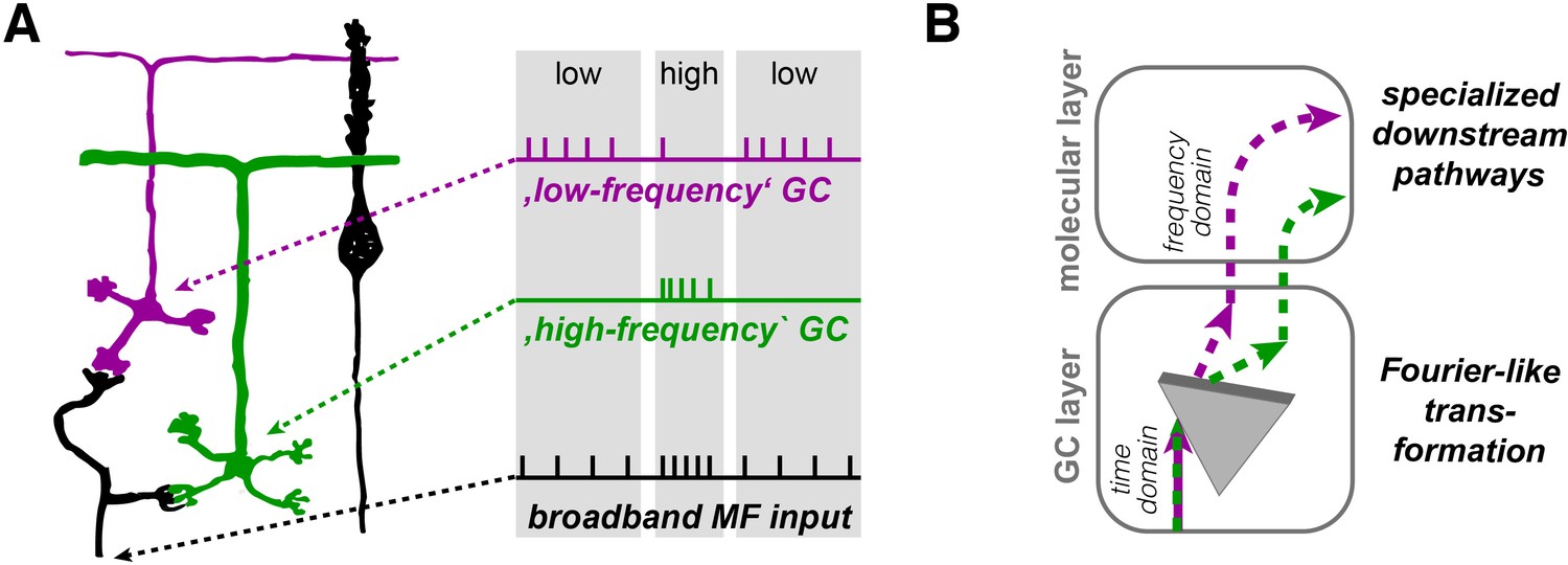
Illustration of the concept of Fourier-like transformation in the cerebellar cortex.
(A) Illustration of a broadband MF input conveying a sequence of low, high, and low firing frequency. Inner-zone GCs will preferentially fire during high-frequency inputs (‘high-frequency’ GC) and outer-zone GCs during low-frequency inputs (‘low-frequency’ GC). (B) Schematic illustration of the signal flow through the cerebellar cortex. The Fourier-like transformation in the GC layer is illustrated as an optical prism separating the spectral components on the MF input. Thereby, the MF signal in the time domain is partially transformed into the frequency domain and sent to PCs via specialized signaling pathways in the molecular layer.
Additional files
Download links
A two-part list of links to download the article, or parts of the article, in various formats.
Downloads (link to download the article as PDF)
Open citations (links to open the citations from this article in various online reference manager services)
Cite this article (links to download the citations from this article in formats compatible with various reference manager tools)
Gradients in the mammalian cerebellar cortex enable Fourier-like transformation and improve storing capacity
eLife 9:e51771.
https://doi.org/10.7554/eLife.51771


