Emergence of social cluster by collective pairwise encounters in Drosophila
- University of Science and Technology of China, China
- Institute of Biophysics, Chinese Academy of Sciences, China
- University of Chinese Academy of Sciences, China
- Capital Medical University, China
Figures
Figure 1 with 9 supplements
Spontaneous clustering of wild-type flies exhibits distinct spatial features.
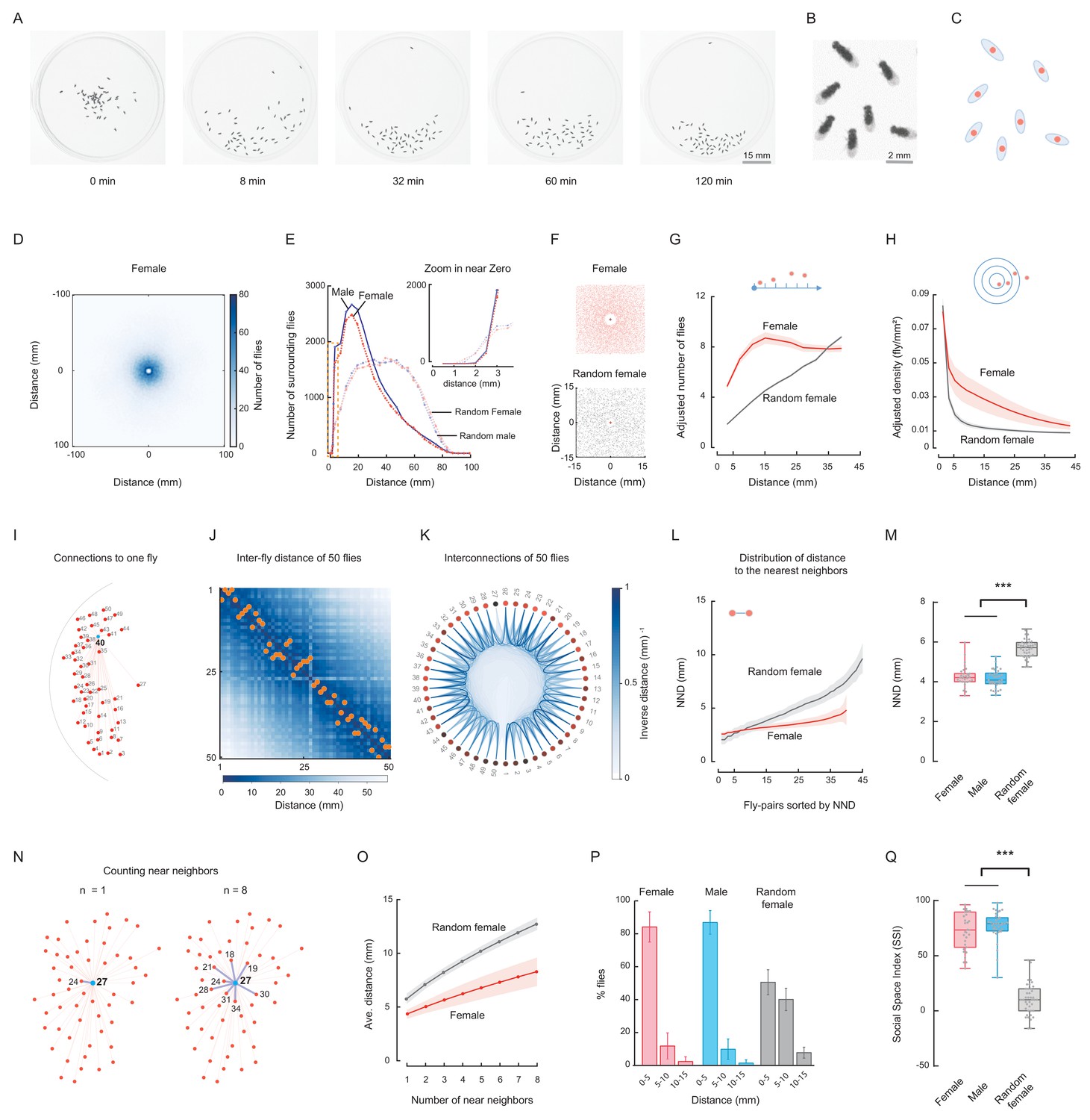
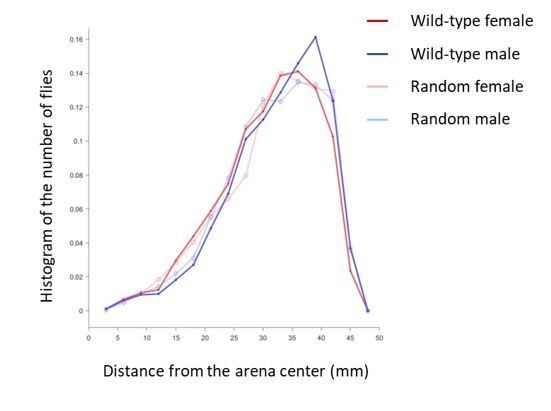
(A) Representative images show the distribution of a group of Canton-S (CS) male flies at the indicated time points. Figure 1—video 1. (B) Enlarged view showing the distribution of six flies in the last image of (A). (C) Representation of flies in (B) by their centres of body mass. (D) Image showing the merged distribution of all surrounding flies in 31 arenas with female CS flies. The origin was the aligned centres of each reference fly. Figure 1—video 2. (E) Quantification of distributions of merged surrounding flies at a distance from the centre. Dark red: CS female; dark blue: CS male; light red: random female (RF); light blue: random male (RM). N = 31, 35, 44 arenas. The insert plot on the left shows an enlarged view of the region near zero. (F) Images showing the enlarged views of the merged distribution of surrounding flies near the origin in wild-type female flies (up) and random female flies (bottom). N = 10 arenas. (G) Distributions of the area-adjusted number of surrounding flies over distance in female (red) and random female flies (grey). The bold lines indicate the average values over all arenas of the same type of fly, with the shaded areas indicate values within one s.e.m (N = 31, 40). (H) Distributions of the density of surrounding flies over distance in female and random female flies. The bold lines indicate the averaged values over all arenas for the same types of fly, with the shaded areas indicate values within one standard deviation (N = 31, 40). (I) Illustration of the measurements of all possible distances from one fly (#40) to others in the arena. Red dots represent individual flies, and numbers indicate their IDs. (J) Matrix of inter-fly distances between all 50 flies in the fly group in (I). The colour bar indicates the distance values. Orange dots marked the positions of shortest distance along each column, resulting in the NND and corresponding nearest neighbour of each fly on the bottom. All flies were females. (K) Circular representation of distance relationship between all 50 flies in (J). The intensities of the blue arcs connecting two flies correspond to the inverse distances between them. (L) Distributions of sorted NNDs of female and random female flies. Bold lines indicate the averaged distribution curve of sorted NNDs over all arenas, with the shaded areas indicate values within one standard deviation. N = 31, 40 arenas. (M) Distribution of the averaged NNDs of all flies in an arena. The flies were female (red), male (blue) and random female flies (grey), in 31, 35 and 40 arenas, respectively. (N) Illustration the first (left) and up to eighth (right) nearest neighbours of the designated reference fly (#27) in a group. Numbers indicate the fly IDs of the identified near neighbours. (O) Distribution of the mean multi-neighbour distances over the number of near neighbours. First the averaged n-near neighbour distance of all flies in an arena was calculated, then the distance values were averaged over all arenas (bold lines). The shaded areas indicate values within one standard deviation. Red indicates female flies and grey indicates random female flies. N = 31 and 40 arenas. (P) Histogram of flies with NNDs in the indicated ranges of distance, with bin 1 = 0–5 mm, bin 2 = 5–10 mm, and bin 3 = 10–15 mm. The types of flies were female (red), male (blue) and random female (grey). N = 31, 35 and 40 arenas, respectively. (Q) Social Space Index was calculated from (P) by subtracting the value of bin2 from that of bin1 in each arena. N = 31, 35, 40 arenas for female (red), male (blue) and random female (grey), respectively. In a box and whisker plot, the scatter points show all data points, the box includes the 25th to 75th percentile, the whiskers mark minimum and maximum, and the middle line indicates the median of the data set. ***: p<0.001 (one-way ANOVA followed with Tukey’s post hoc test for multiple comparisons).
-
Figure 1—source data 1
Figure 1M, P-Q source data and related summary statistics.
- https://cdn.elifesciences.org/articles/51921/elife-51921-fig1-data1-v2.zip
Figure 1—figure supplement 1
Experimental setup.
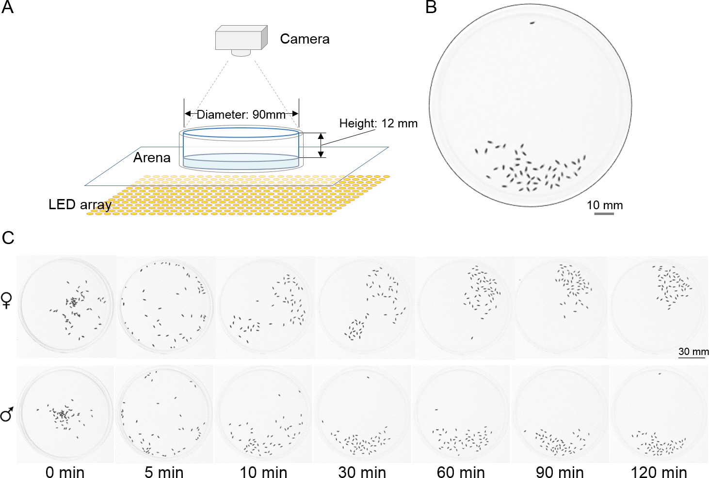
(A) Schematic of the setup for the social cluster paradigm. 50 flies in the circular arena were illuminated by a LED array from bottom and their distributions were recorded by a camera or camcorder. Light blue indicates the agarose pad on the bottom of the arena. (B) A representative image showing a cluster of male wild-type flies at 60 min. (C) Representative sequences of images showing distribution patterns of CS female (top) and male (bottom) flies at the indicated time points. At time zero, briefly anaesthetised flies were transferred to the centre regions of the arenas.
Figure 1—figure supplement 2
Merged distribution of surrounding flies.
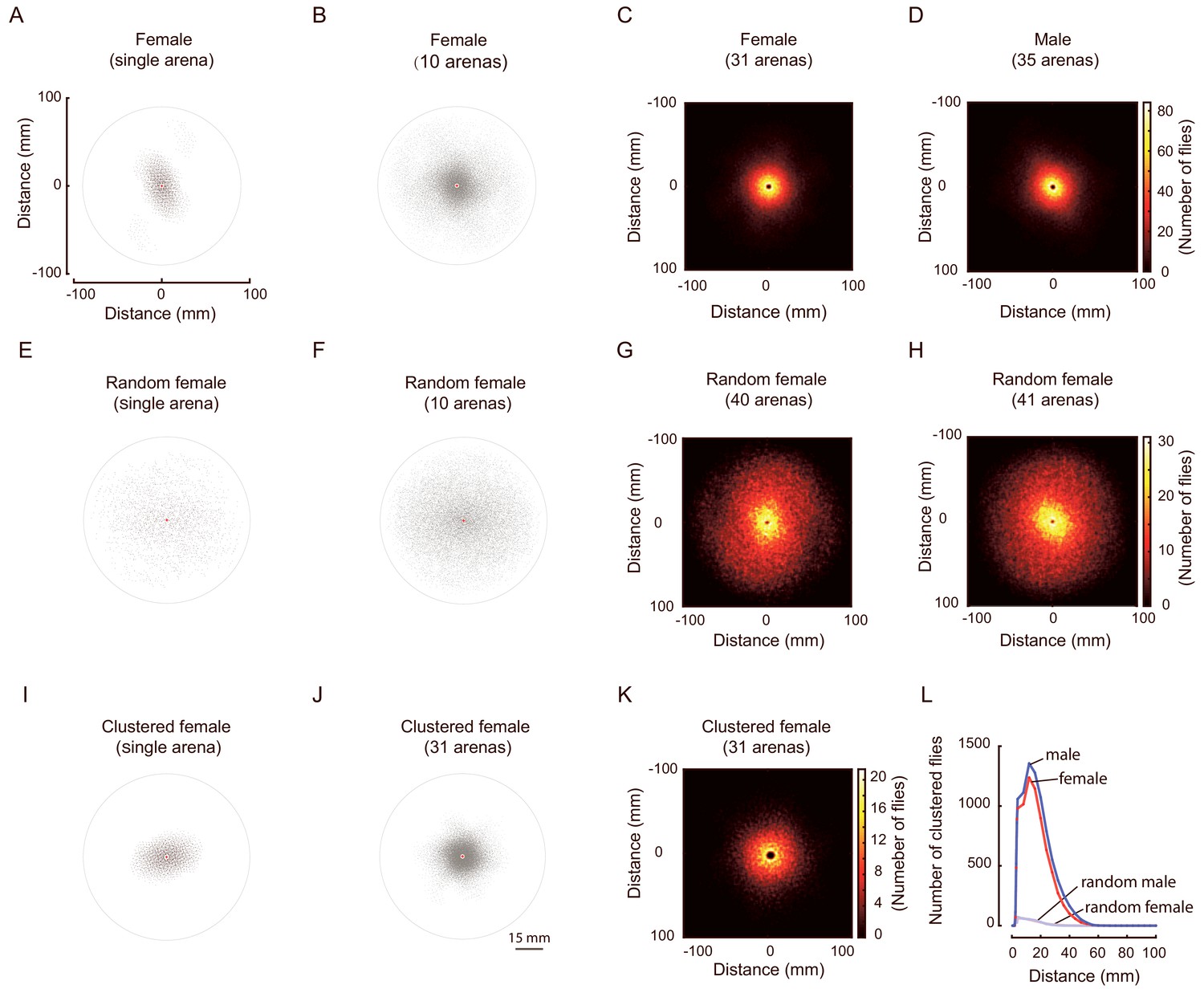
(A) An example of the distribution of superimposed surrounding flies from one arena with wild-type female flies. The plot was generated by superimposing the all surrounding flies for all flies in that arena, with each fly serving as the reference fly in turn. The origin point (red-cross) is the aligned body centre of the reference flies. The thin circle marks a distance of 90 mm from the origin. (B) A plot combining the superimposed surrounding flies of 10 arenas with wild-type female flies. (C, D) Heat map representations of the merged distributions of surrounding flies of females (C, 31 arenas) and males (D, 35 arenas). The colour bar indicates the number of flies. Data in (C) were replicated from Figure 1D. (E, F) Plots presenting the merged distributions of surrounding flies from a single arena (E) and 10 arenas (F) in random females. (G, H) Heat map representations of the merged distribution of surrounding flies of random females (G, 40 arenas) and random males (H, 41 arenas). (I) Plot showing the distribution of superimposed surrounding flies of a cluster from an arena of wild-type females. (J) Plots showing the merged distributions of surrounding flies of the same clusters from 31 arenas of wild-type females. For each arena, both reference flies and surrounding flies were from the same clusters. (K) A heat map image representation of the merged distribution of surrounding flies within clusters. Data were clustered female flies from 31 arenas. (L) Quantification of the distributions of merged surrounding flies over a distance from the origin in female (dark red), random female (pink), male (dark blue) and random male (light blue) flies. N = 31, 40, 35, 41 arenas, respectively. For (I)-(L), the criterial set for clustering is 5 (see Figure 2 for more).
-
Figure 1—figure supplement 2—source data 1
Figure 1—figure supplement 2 source data related summary statistics.
- https://cdn.elifesciences.org/articles/51921/elife-51921-fig1-figsupp2-data1-v2.mat
Figure 1—figure supplement 3
Quantification of area-adjusted number of surrounding flies and density of surrounding flies.
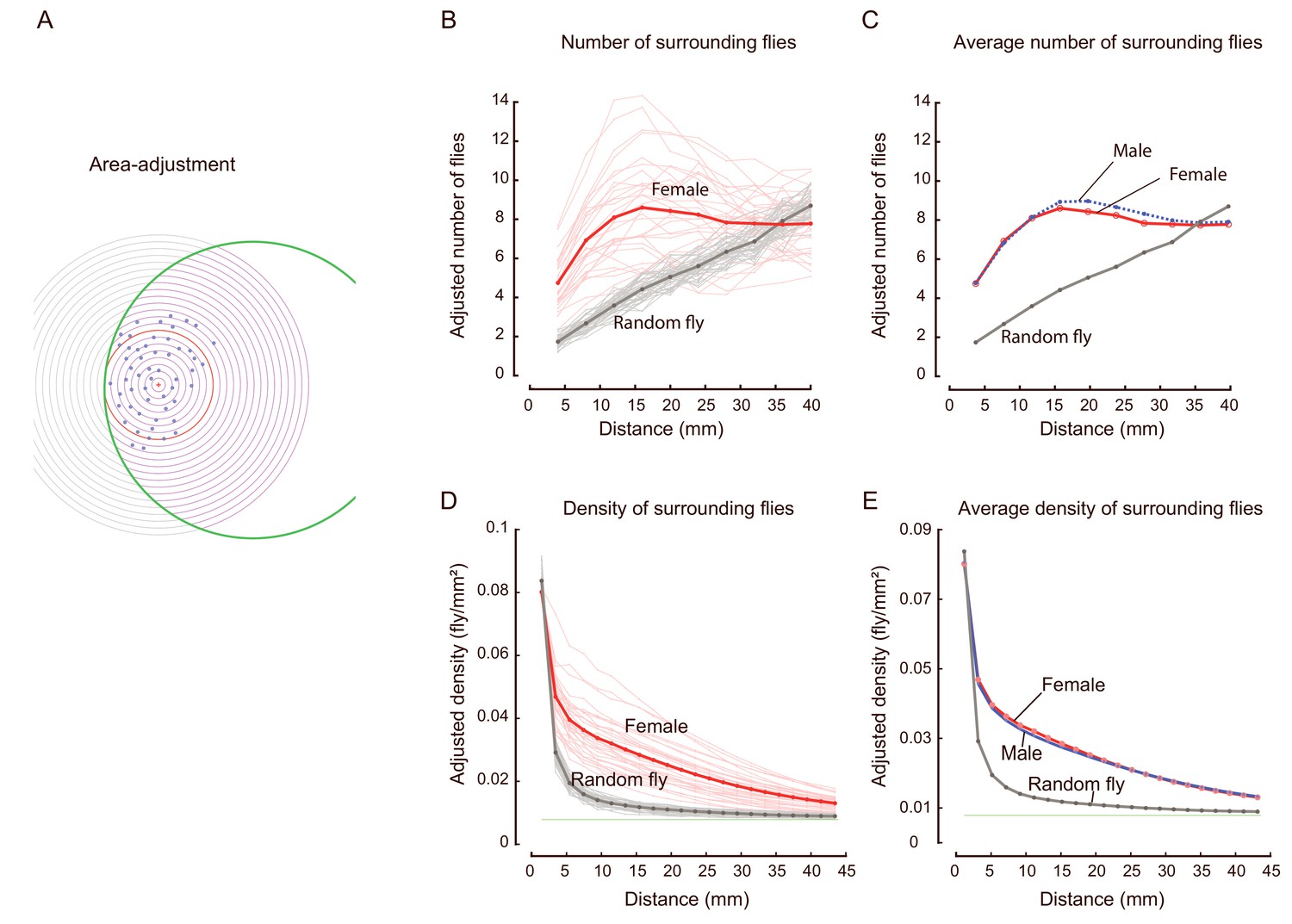
(A) Schematic for making adjustments to the area when calculating the number of surrounding flies and the density of surrounding flies for a reference fly. The red-cross represents the reference fly, blue dots indicate its surrounding flies, and the green circle indicates the edge of the arena. Thin concentric circles indicate various distances from the reference fly. The bold red circle indicates the distance after which the area-correction was necessary. The red area of the intersection of the green and a thin-lined circle is the actual area (Areain) allowed for the flies to occur, whereas the grey area outside of the intersection of the green and the thin-lined circle (Areaout) would not contain flies, and would therefore need to be compensated. Cumulative distribution function of area-adjusted numbers of surrounding flies vs. a designated distance (from a reference fly)=number of surrounding flies (with that distance)*(Areaout + Areain)/Areain. From the cumulative distribution functions, the probability density functions in (B) and (C) were derived. Density of surrounding flies (within a designated distance from a reference fly)=number of surrounding flies (within that distance)/Areain. (B) Distribution of the area-adjusted number of surrounding flies over distance. Each thin line represents the average over all flies (each serving as the reference fly once) in one arena, the bold lines represent the average over all arenas of a type of flies. Red and grey indicate female and random flies; the number of arenas was 31 and 40, respectively. (C) Averaged distributions of the area-adjusted number of surrounding flies from all arenas of each type of flies, female (red), male (blue) and random female (grey); the number of arenas was 31, 35, and 40, respectively. (D) Distribution of the density of surrounding flies over distance. Each thin line represents the average of all flies (each serving as the reference fly once) in one arena. The bold lines represent the average of all arenas of the designated type of flies: female (red), male (blue) and random female (grey). The number of arenas was 31 and 40 for females and random females, respectively. The horizontal green line near 0.01 indicates the theoretical limit of density when distance reached the diameter of the arena. (E) Averaged distribution of the density of surrounding flies from all arenas, for each type of fly; female (pink), male (blue) and random female (grey); the number of arenas was 31, 35, and 40, respectively. Data in (B–C) were replicated in Figure 1G–H.
-
Figure 1—figure supplement 3—source data 1
Figure 1—figure supplement 3 source data related summary statistics.
- https://cdn.elifesciences.org/articles/51921/elife-51921-fig1-figsupp3-data1-v2.mat
Figure 1—figure supplement 4
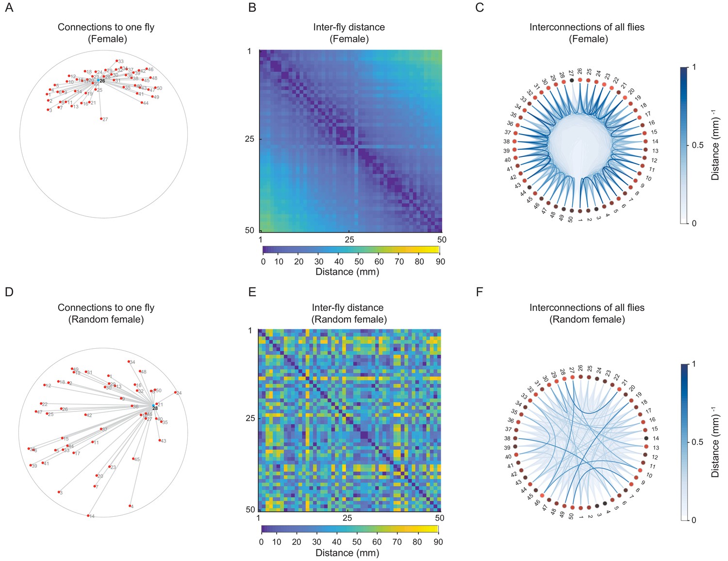
Estimating inter-fly connections via distance matrices.
(A) Example plot showing the inter-fly connections from a reference fly (ID: 26) to all other flies in an arena of wild-type females (CS). Red dots represent individual flies, the number near each dot indicates the fly ID, and grey lines represent connections. The grey circle indicates the edge of the arena. (B) A matrix showing distances between all possible pairs from the group in (A). The colour bar indicates the distance values. (C) Circular visualisation of inter-fly connections between all flies in (A). The numbers outside indicate fly IDs. The colour of each arc connecting two flies is correlated to the inverse distance between them; therefore, a darker colour indicates a shorter distance (and a stronger connection). (D) Example plot showing the inter-fly connections from a reference fly (ID: 28) to all other flies in an arena of random female flies. The colours and labels are the same as in (A). (E) Matrix showing distances between all possible pairs from the group in (D). (F) Circular visualisation of inter-fly connections between all flies in (D). The colours and labels are the same as in (C). Data in (A–C) were replicated in Figure 1I–K.
-
Figure 1—figure supplement 4—source data 1
Figure 1—figure supplement 4 source data.
- https://cdn.elifesciences.org/articles/51921/elife-51921-fig1-figsupp4-data1-v2.mat
Figure 1—figure supplement 5

Analysing the distribution of Nearest Neighbour Distance.
(A) Representative plot showing all of the nearest neighbours in an arena of females. The red dots mark all flies, the blue circle represents a reference fly, the green circle indicates its nearest neighbour, the thick red line indicates the shortest among the distances from the reference fly to its surrounding flies (thin red lines). The bold blue lines connect all pairs of nearest neighbours. (B) Arrangement of all NNDs in (A) from small to large. Connecting the top red dots formed a curve reflecting distribution of NNDs within this arena. The two numbers under the vertical blue lines indicate the fly IDs of each pair. (C) The distribution of sorted NNDs in female (red) and random female (grey). Each thin line represents the distribution curve of sorted NNDs from one arena, the bold lines represent the average NNDs of all arenas (N = 31 and 40). (D) Averaged distributions of sorted NNDs in female (red), male (blue) and random female (grey) (N = 31, 35, and 40 respectively). (E) Comparing the averaged minimal NNDs. Data represent the distribution of the minimal NND of each arena in females (red), males (blue) and random females (grey) (N = 31, 35, and 40, respectively). Data in (C) were replicated in Figure 1O. In a box and whisker plot, the scatter points show all data points, the box includes 25th to 75th percentiles, and the middle line indicates the median of the data set. ***: p<0.001 (one-way ANOVA followed by Tukey’s post hoc test for multiple comparisons).
-
Figure 1—figure supplement 5—source data 1
Figure 1—figure supplement 5A-E source data related summary statistics.
- https://cdn.elifesciences.org/articles/51921/elife-51921-fig1-figsupp5-data1-v2.zip
Figure 1—figure supplement 6
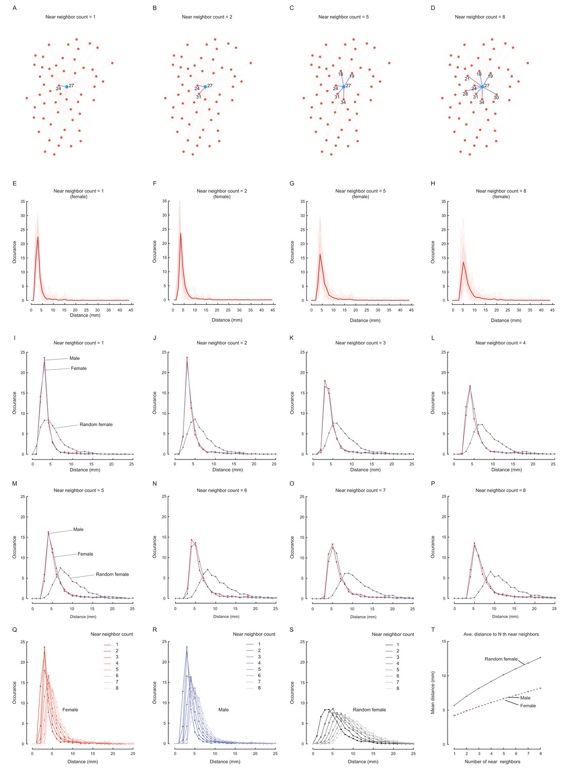
Characterisation of averaged distance to multiple near neighbours.
(A–D) Plots of a group of flies from an arena showing examples to calculate the distances from a reference fly (blue dot, ID: 27) up to its 1st (A), 2nd (B), 5th (C) and 8th (D) nearest neighbours, referred as 1-, 2-, 5-, and 8-th near neighbour distances. For this arena, the N-th near neighbour distance was a collection of the averaged values over specific number of near neighbours of each reference flies (the neighbour count, N = 1–8). (E–H) The distributions of multi-neighbour distances in wild-type females. The thin lines represent the individual arenas and the bold lines represent averaged values over all arenas for each neighbour count: 1 (E), 2 (F), 5 (G) and 8 (H). (I–P) Comparing the distributions of averaged multi-neighbour distances in female (red), male (blue) and random females (grey). (Q–S) Comparing distributions of averaged multi-neighbour distances for different neighbour counts. The shades of colours from dark to light correspond to the neighbour count from 1 to 8. The coloured lines indicate female (red, (Q), male (blue, (R) and random female (grey, (S). (T) A plot showing the tendency of averaged multi-neighbour distances as the neighbour counts increased. The coloured lines indicate females (red), males (blue) and random females (grey). In this figure, the number of arenas was N = 31, 35, and 40 for females, males and random females, respectively. The values in (E)-(S) were the numbers of relevant events.
-
Figure 1—figure supplement 6—source data 1
Figure 1—figure supplement 6 source data related summary statistics.
- https://cdn.elifesciences.org/articles/51921/elife-51921-fig1-figsupp6-data1-v2.mat
Figure 1—figure supplement 7
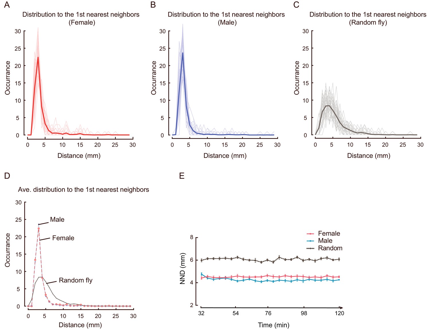
Distribution of distance to the 1st nearest neighbours in wild-type flies and simulated flies.
(A–D) Histograms of the distance to the 1st nearest neighbours (same as NND) in female (A, red), male (B, blue), random females (C, grey) and the average of them (D). (A) and (D) were replicated of Figure 1—figure supplement 6E and I. In (A–C), the thin lines show histograms of all NNDs in each arena, while thick lines show averaged histograms of NNDs over all arenas of each types of fly. The coloured lines in (D) are replicas of the thick lines in (A–C). N = 31, 35, and 40 arenas. (E) Changes of averaged NNDs over the period of 32–120 min in female (red), male (blue), random flies (grey) (N = 21, 22, 24 arenas). Error bars indicate s.e.m.
-
Figure 1—figure supplement 7—source data 1
Figure 1—figure supplement 7E source data and related summary statistics.
- https://cdn.elifesciences.org/articles/51921/elife-51921-fig1-figsupp7-data1-v2.zip
Figure 1—video 1
supplement to Figure 1.
A representative video showing the process of social clustering in wild-type (CS) female flies. The video covers the first 0–23 min of observation. The recording frame rate was 25 fps, sped up 125×.
Figure 1—video 2
supplement to Figure 1D.
A video illustrating how to obtain the superimposed distribution of surrounding flies in order to quantitatively analyse the spatial distribution of an arena (and a genotype).
Figure 2 with 10 supplements
Social cluster represents a well-structured network.
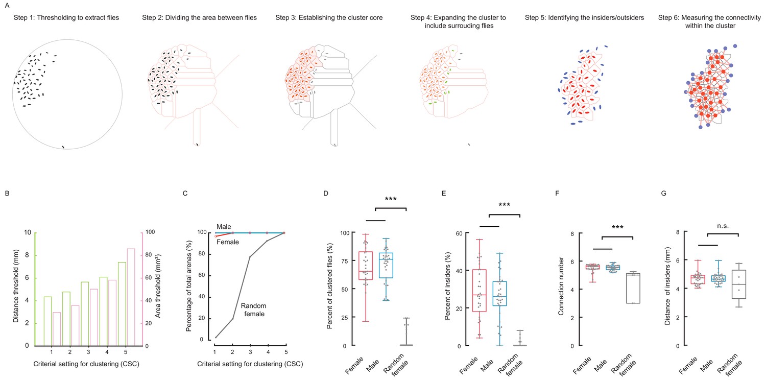
(A) A six-step procedure to automatically reconstruct a cluster from a group of flies in two dimensional space. Step 1: Using digital image processing methods to extract the pixels of each fly from a raw image and calculating the geometric properties of the pixel set of that fly. Step 2: Dividing the area between all flies and the edge of arena. The divided area surrounding each fly is designated as its residing area. Step 3: Establishing the basic cluster by combining flies whose residing areas are smaller than an area threshold. Each red ellipse indicates a fly incorporated by the cluster; the corresponding pink shaded area indicates its residing area. Step 4: Repeatedly expanding the cluster to include surrounding flies (green) within a threshold distance. The leftover fly was coloured grey. Step 5: In the resultant cluster, identifying the insiders (red) and outsiders (blue). Step 6: Quantifying the local regularity of the cluster. Figure 2—video 1. (B) Showing the area threshold and distance threshold (as a set) to reconstruct clusters in (A). Five criterial settings for clustering (CSC), with stringency from high to low, were defined and evaluated in the following panels. (C) Comparing the percentages of arenas formed a cluster under the CSC from 1 to 5. N = 31, 34, 40 arenas for female, male and random female flies, respectively. (D) Average percentage of clustered flies (CSC = 2). (D) Average percentage of clustered flies (of total flies in an arena) (CSC = 2). (E) Average percentage of insiders of total flies (CSC = 2). (F) Average number of connections from an insider to its contiguous neighbours (CSC = 2). (G) Average distance of an insider to its contiguous neighbours (CSC = 2). N = 31, 34, 40 arenas in (C–E) and N = 31, 34, five arenas in (F–G) for female, male and random female flies, respectively. Data in (D, E) were part of Figure 2—figure supplement 2A and C; Data in (F,G) were part of Figure 2—figure supplement 3F and G. In a box and whisker plot, scatter points show all data points, the box includes 25th to 75th percentile, the whiskers mark minimum and maximum, and the middle line indicates the median of the data set. ***: p<0.001 (one-way ANOVA followed with Tukey’s post hoc test for multiple comparisons).
-
Figure 2—source data 1
Figure 2D-G source data and related summary statistics.
- https://cdn.elifesciences.org/articles/51921/elife-51921-fig2-data1-v2.zip
Figure 2—figure supplement 1
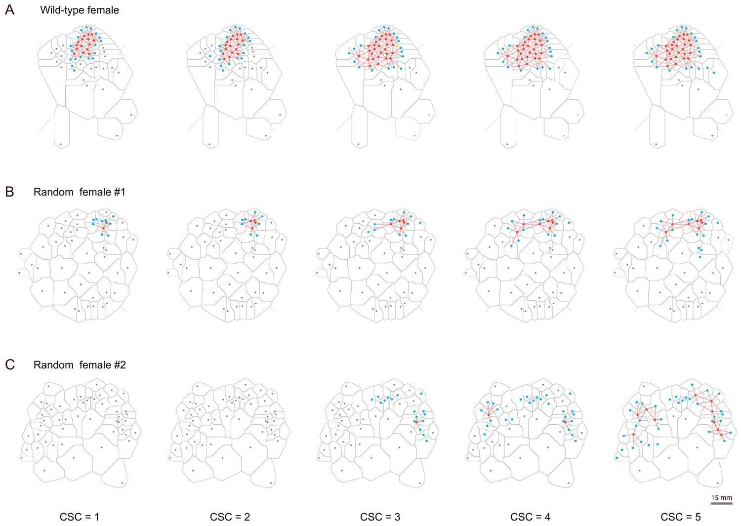
Patterns of clusters reconstructed with different clustering criteria.
(A–C) Examples of clusters formed by wild-type females (A) and random females (B and C). In a single arena, more flies were assigned into the cluster as the stringency decreased (from left to right). The CSC for building each cluster was indicated at the bottom. Red dots: cluster insiders; blue dots: cluster outsiders; grey dots: flies not associating with a cluster; red lines: connections of insiders. (A) Patterns of changing clusters in wild-type females. (B) Patterns of changing clusters in random females. This arena exhibited cluster formation across all clustering criteria (CSC = 1 ~ 5), among all arenas with random flies. (C) Patterns of changing clusters in random females. This arena exhibited the highest number of flies joining clusters at the relaxed condition (CSC = 5), among all arenas with random flies.
Figure 2—figure supplement 2
Exploring the settings of cluster criteria on cluster reconstruction.
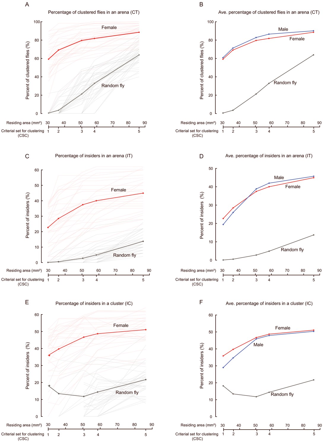
(A) Comparing the CT values (percent of clustered flies in an arena) evaluated with different settings of criteria. Thin lines indicate the CT values of each arena; the thick lines show the averaged CT values of all arenas. Red: female, N = 31 arenas; grey: random females, N = 40 arenas, respectively. (B) Averaged percentage of clustered flies in females (red, N = 31 arenas), males (blue, N = 35 arenas), and random females (N = 40 arenas). Data for females and random females were replicated from (A). (C) Comparison of IT values (the percentage of insiders within an arena) evaluated with different sets of criteria. Thin lines indicate the values of each arena, the thick lines show the average IT values of all arenas. Red: female, N = 31 arenas; grey: random females, N = 40. (D) Averaged percentage of insiders for different types of fly: female (red, N = 31 arenas), male (blue, N = 35 arenas), and random female (grey, N = 40 arenas). Data for females and random females were replicated from (C). (E) Comparison of IC values (the percentage of insiders of the clustered flies in an arena) evaluated with different sets of criteria. Thin lines indicate the values of each arena; the thick lines show the average IT values of all arenas. The number of arenas for CSC from 1 to 5 were: 29, 30, 30, 30 and 30 in female (red), and 1, 5, 22, 31 and 40 in random females (grey), respectively. In random flies, quantification of the first two data points of the averaged IC values was tenuous, because only a few arenas containing identified clusters under high stringency (when CSC was 1 and 2, the number of clusters was 1 and 5, respectively). (F) Averaged percentage of insiders of clustered flies, for different types of flies. The number of arenas in males for CSC from 1 to 5 were: 33, 34, 35, 35 and 35, respectively. Data for females and random females were replicated from (E).
-
Figure 2—figure supplement 2—source data 1
Figure 2—figure supplement 2 source data and related summary statistics.
- https://cdn.elifesciences.org/articles/51921/elife-51921-fig2-figsupp2-data1-v2.mat
Figure 2—figure supplement 3
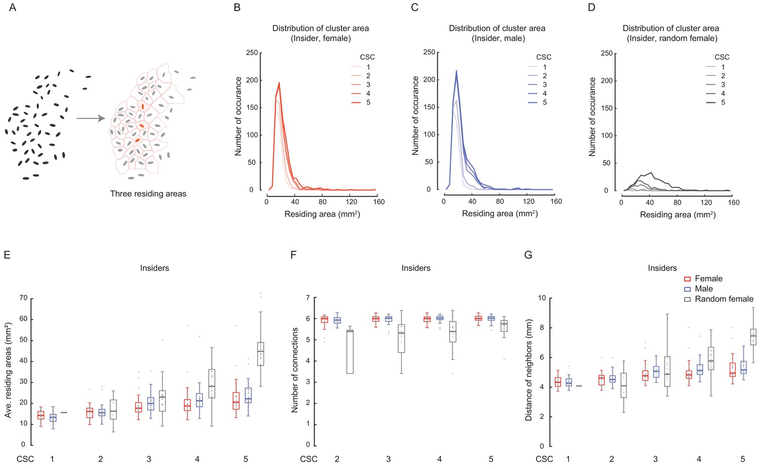
Characterising the properties of identified clusters.
(A) Illustration of the residing areas of three cluster insiders. Each pink region including an insider was separated automatically with red lines, the area of which was designated as the residing (or inhabited) area of that fly. (B–D) Distributions of the averaged residing areas of insiders in females (B), males (C) and random females (D) evaluated with stringency for cluster reconstruction from high to low. The five shades of each colour from light to dark correspond to CSC from 1 to 5. The numbers of arenas were 29–31 (female) and 33–35 (male). For random females, the numbers of arenas were 1, 5, 22, 31 and 40 for CSC from 1 to 5, respectively. (E) Comparing the distributions of the averaged residing areas of insiders under different criterial settings. The number of arenas for each type of flies were the same as in (C–E). (F) Averaged number of connections of insiders with contiguous neighbours under clustering criterial settings from 2 to 5. The number of arenas were 31 in females (red), 34–35 in males (blue). In random female flies (grey), the number of arenas were 5, 22, 31 and 40 for CSC from 2 to 5, respectively. (G) Averaged distance between insiders with contiguous neighbours under cluster criterial settings from 1 to 5, in females (red), males (blue) and random females (grey) flies. The number of arenas for each type of fly was the same as in (B–D).
-
Figure 2—figure supplement 3—source data 1
Figure 2—figure supplement 3 source data and related summary statistics.
- https://cdn.elifesciences.org/articles/51921/elife-51921-fig2-figsupp3-data1-v2.mat
Figure 2—figure supplement 4
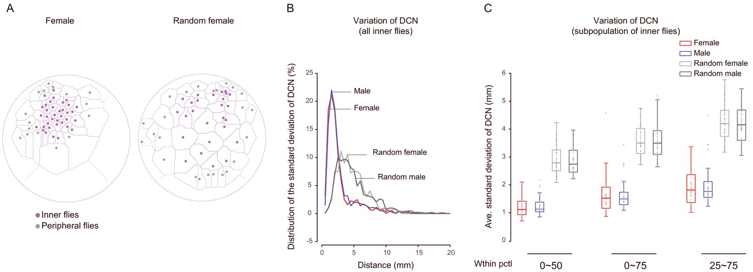
Analysing the variation within distances of the contacting neighbours.
(A) Example arenas showing the peripheral (grey) and inner (purple) flies. The flies were classified based on whether they bordered with the edge of arena. Left: an arena with wild-type females; right: an arena with random females. (B) Histogram of the standard deviations of the distances of contiguous neighbors (DCN) of all inner flies. The number of flies was: 883 (female, red), 1013 (male, blue), 911 (random female, light grey) and 917 (random males, grey). (C) Quantification of the variation of the distance of contiguous neighbors in subpopulations. In each arena, the standard deviations of DCN falling into an indicated range (within percentile of 0 ~ 50 th, 0 ~ 75 th or 25th ~ 75 th) were averaged to generate a data point representing the arena. The number of arenas was: 30 (female, red), 35 (male, blue), 40 (random female, light grey) and 41 (random males, grey).
-
Figure 2—figure supplement 4—source data 1
Figure 2—figure supplement 4 source data and related summary statistics.
- https://cdn.elifesciences.org/articles/51921/elife-51921-fig2-figsupp4-data1-v2.zip
Figure 2—figure supplement 5
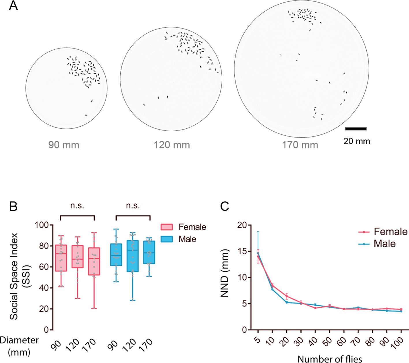
Social clustering is independent of arena size.
(A) Representative images showing the distribution of flies in arenas of different diameters. The number of tested flies was 50. (B) SSIs of flies tested in the arenas with the indicated diameter (N = 13–20 arenas). (C) Nearest neighbour distance (of various numbers of wild-type flies in arenas of 90 mm diameter (N = 4–8 arenas). All experimental conditions are indicated with the plots. In a box and whisker plot, scatter points show all data points, the whiskers mark minimum and maximum, and the middle line indicates median of the data set. Error bars in (C) show s.e.m. n.s. (p>0.05) indicates not significant (Student’s t-test for two-group comparisons, one-way ANOVA followed with Tukey’s post hoc test for multiple comparisons).
-
Figure 2—figure supplement 5—source data 1
Figure 2—figure supplement 5B-C source data and related summary statistics..
- https://cdn.elifesciences.org/articles/51921/elife-51921-fig2-figsupp5-data1-v2.xlsx
Figure 2—figure supplement 6
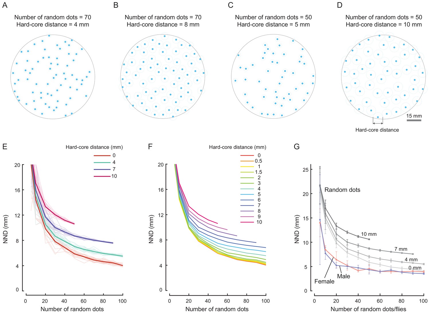
Comparing spatial patterns of random dots with that of real flies.
(A) Example of spatial distribution of a group of 70 simulated random dots in an arena. The minimal allowed distance (D; i.e., hard-core distance) between random dots was 4 mm. Blue dots represent random dots, light blue circles marked the impermissible regions of random dots. The grey circle indicates the edge of the arena (diameter = 90 mm). For simplification, the random dots were allowed to stay close to the edge of arena, regardless of their hard-core distance. (B) Same as (A) except that the minimal allowed distance between random dots was 8 mm. (C, D) Examples of spatial distribution of 50 random dots with hard-core distances of 5 mm (C) and 10 mm (D). (E) Distributions of NND over the size of a group in an arena. Different colours indicate different minimal allowed distances between random dots. The thin lines indicate individual distributions; the bold lines indicate the averaged value for each group with the same hard-core distance (N = 20 arenas for each hard-core distance). (F) Averaged NNDs over group size for minimal allowed distances ranging from 0 mm to 10 mm (N = 20 arenas for each hard-core distance). (G) Comparison of the averaged NNDs over group size in females (red, N = 4–8 arenas), male (blue, N = 4–8 arenas) and random dots (grey, N = 20 arenas. Average NNDs of random dots were replicated from (E), and the values for the wild-type flies were replicated from Figure 2—figure supplement 5C. Different shades of grey indicate random dots with hard-core diameters of 0, 4, 7, and 10 mm. Error bars show s.e.m.
-
Figure 2—figure supplement 6—source data 1
Figure 2—figure supplement 6 source data and related summary statistics.
- https://cdn.elifesciences.org/articles/51921/elife-51921-fig2-figsupp6-data1-v2.mat
Figure 2—figure supplement 7

A simple model of clustering by the combined effects of global attraction and local repulsion in a two-dimensional space.
(A) Distance functions of attractive and repulsive forces by individual flies. To simplify the comparison, the area under each curve was one for the distance range from −20 to 20 mm. The blue curve is an arbitrarily-selected attraction profile defined by a Gaussian function, Fa = a*EXP(−(distance-µ)^2/ (2*σ^2))/ (σ*sqrt(2*pi)), with µ = 0 mm, σ = 5 mm and a = 1.0001. The light blue curve is another arbitrarily-selected attraction profile (Fa = b/4, when distance ≤2 mm; Fa = b/distance2, when distance >2 mm; b = 0.5263 mm). The red curve is a repulsive force resembling a step function (Fr = 0.1, when distance <5 mm; Fr = 0, when distance ≥5 mm). (B) Illustration of the summation of the attractive and repulsive forces on a fly. The small circles represent three flies establishing a small cluster and the hexagrams represent the testing fly. Left: attractive forces (light blue arrows) and their combined effect (blue arrow) perceived by the testing fly. Middle: repulsive forces (orange red arrows) and their combined effect (red arrow) perceived by the testing fly. Right: the net force (purple arrow) perceived by the testing fly. (C) The distributions of net force within a field of a narrow stripe. The upper panel shows the net forces that are repulsive (red). The lower panel shows the net forces that are attractive (blue). The relative strength and direction of the force vector at each randomly-selected location are represented by an arrow. (D) Computing the net force along a horizontal line (y = 0) in (C) with varying strengths between attractive function, Fa (distance), and repulsive function, Fr (distance). The net force: F = Fa + C*Fr. Left: the force of repulsion (red curves) increases as C factor increases. Right: the net force (green curves) switches from repulsion (<0) to attraction (>0) after a critical distance, when the C factor is sufficiently large (C ≥ 2). A positive value of net force indicates attraction, whereas a negative value indicates repulsion. Blue curve: attractive force. (E) Part of a force field generated by a set of nine flies. At each illustrated location, the direction of force is depicted by an arrow, while the strength of force is colour-coded. Red arrows indicate repulsion while arrows of other colours indicate attraction. Owing to the high dynamic range of the dataset of attractive forces, the colours of attraction arrows represent the percentile ranges in this dataset, instead of the force values. In (B–E), all distances between nearby flies in a set are 5 mm. The attraction functions used were the Gaussian function in (A); the other attraction function shown in (A) also produced similar results. In (C–E), the small cluster contains a set of nine flies as shown in (E). The C factors are 10 and 2 for (C) and (E), respectively.
Figure 2—figure supplement 8
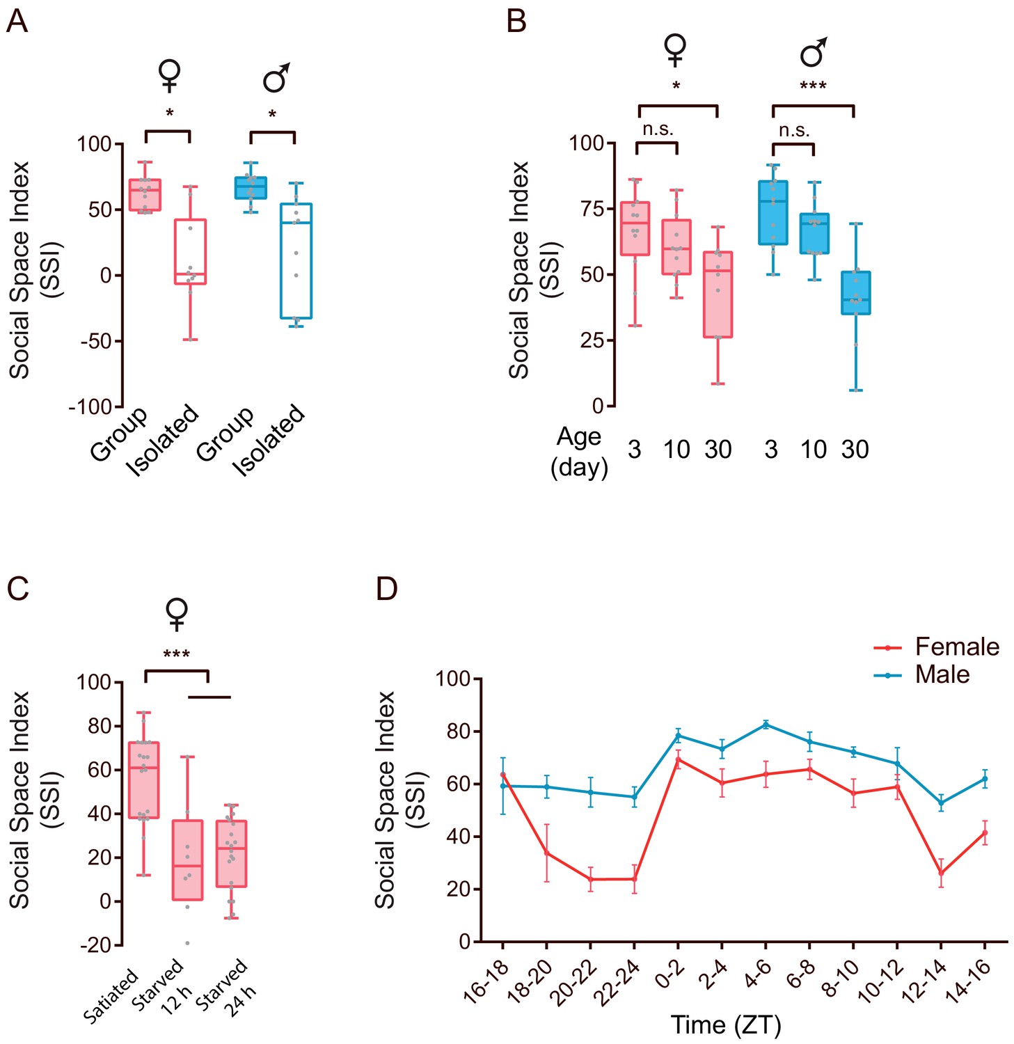
Social experience, physiological state, age and circadian rhythm modulate social clustering in wild-type flies.
(A) Social isolation adversely affected social clustering. ‘Group’ indicates flies raised together after eclosion; ‘isolation’ indicates newly hatched flies reared alone for 7 days before the behavioural test (N = 10–12). (B) SSI representing the aggregation tendency of CS flies with different ages. The flies were tested 3 days, 10 days and 30 days after eclosion. Older flies exhibited decreased social clustering. (N = 10–12). (C) Starved CS flies exhibited decreased SSIs. Female flies were starved for 12 or 24 hr (N = 8–20). (D) The circadian oscillation of the tendency to form social clusters in male and females (N = 6–15). All experimental conditions are indicated with the plots. In a box and whisker plot, scatter points show all data points, the box includes 25th to 75th percentiles, the whiskers mark minimum and maximum, and the middle line indicates the median of the data set. N indicates the number of arenas. Error bars indicate s.e.m. n.s. indicates non-significance (p>0.05); *: p<0.05, ***: p<0.001 (Student’s t-test).
-
Figure 2—figure supplement 8—source data 1
Figure 2—figure supplement 8A-D source data and related summary statistics.
- https://cdn.elifesciences.org/articles/51921/elife-51921-fig2-figsupp8-data1-v2.xlsx
Figure 2—figure supplement 9

Grooming did not affect social clustering.
(A) Representative images show body surfaces of untreated (top) and dusted (middle and bottom) flies. (B) Grooming performance of individual female flies during 2 min trials. Top: untreated wild-type flies (control); bottom: dusted wild-type flies. Various colours indicate individual flies, and the lengths of horizontal bars indicate the durations of individual grooming events. (C) Quantification of the duration of grooming events (N = 5). (D) Comparison of Social Space Index of dusted flies with that of untreated flies. SSI was obtained at 60 min of the trial. (N = 10). All experimental conditions are indicated with the plots. In a box and whisker plot, scatter points show all data points, the box includes the 25th to 75th percentiles, the whiskers mark the minimum and maximum, and the middle line indicates median of the data set. Error bars indicate s.e.m. ***: p<0.001 (Student’s t-test).
-
Figure 2—figure supplement 9—source data 1
Figure 2—figure supplement 9C-D source data and related summary statistics.
- https://cdn.elifesciences.org/articles/51921/elife-51921-fig2-figsupp9-data1-v2.xlsx
Figure 2—video 1
supplement to Figure 2A.
A video showing steps to reconstruct a cluster out of an image of an arena with flies.
Figure 3 with 3 supplements

Dyadic encounter events are the main form of interactions during cluster formation in wild-type flies.
(A) Rapid increase of the cluster size (number of flies) through incorporating more flies during clustering (N = 7 arenas). (B) Total encounter events during the period between 5 and 20 min (N = 5 arenas). (C) The number of encounter events in three stages of cluster growth (N = 5 arenas). (D) Schematic of an encounter event to show the appendage touch-points on the Interactee. Eight touch-points were defined: F (Frontal), L1-L3 and R1-R3 (Legs), R (rear or wings). (E) The proportion of body points touched by an ‘Interactor’ in male flies. Flies are shown in white at the centre and the proportion of each touch point is presented by the length of colour-coded bar. N = 5 arenas, and the number of encounter events = 203, 180, 140 for stages 1, 2 and 3. (F, G) Percentage of behavioural responses of the ‘Interactee’ after touching by the ‘Interactor’, in males (F) and females (G). The ‘Interactee’ used wings (Wing) or legs (Leg) to repel the ‘Interactor’ after being touched. N = 5 arenas, number of events = 471 (male) and 199 (female). (H) Three images from a video sequence showing behaviours by the ‘Interactor’ and ‘Interactee’ during an encounter event. The red dashed line indicates the locomotion trajectory of ‘Interactor’. Figure 3—video 1. (I, J) Behaviour outputs after social encounters in the ‘Interactor’ and ‘Interactee’ in females (I) and males (J). Left panel: percentage of behavioural responses in the three stages; Right panel: percentage of net movement of encountered pairs (all three stages combined, quantified from the left panel). Stay: stay at the original location after encountering. Move: move away after encountering. N = 5 arenas, number of events = 1046 (male) and 474 (female).
-
Figure 3—source data 1
Figure 3A–C, E–G, and I–J source data and related summary statistics.
- https://cdn.elifesciences.org/articles/51921/elife-51921-fig3-data1-v2.zip
Figure 3—figure supplement 1
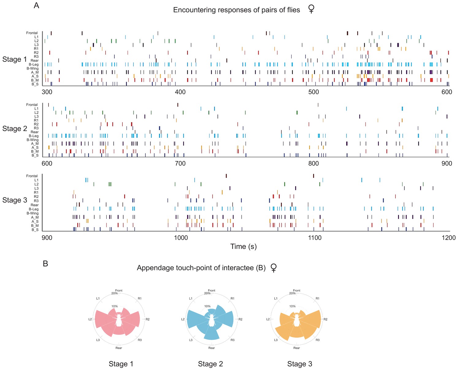
Quantification of touched sites and behavioural outputs of encounters in wild-type female flies.
(A) Timed-event data showing quantification of the details of encounter responses of fly pairs in three stages of cluster development in one arena. Each row indicates a specific type of actions or events, the corresponding labels were as follows: Frontal, L1-3, R1-3 and Rear (appendage touch-points on ‘Interactee’), ‘B_Leg’ and ‘B_Wing’ (touch-evoked responses of ‘Interactee’), ‘A_Move’ or ‘A_Stay’ (‘Interactor’ moving away or staying at the encounter site after encountering), ‘B_Move’ or ‘B_Stay’ (‘Interactee’ moving away or remaining unmoved after encountering). (B) The distribution of touch points on the ‘Interactee’. The flies are shown in white at the centre. The proportion of the number of touches at each touch point is represented by the length of a colour-coded bar (N = 5 arenas).
-
Figure 3—figure supplement 1—source data 1
Figure 3—figure supplement 1B source data.
- https://cdn.elifesciences.org/articles/51921/elife-51921-fig3-figsupp1-data1-v2.xlsx
Figure 3—figure supplement 2
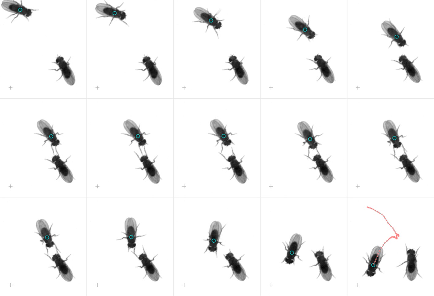
An image sequences of an encounter event in males.
A sequence of frames from a high-speed video showing direct interactions (appendage touches) between a moving fly and a stationary fly. The moving fly is labelled with a green circle on its centre of body mass, and the trace of the centre of mass during the displayed period is plotted as pink dots in the last frame. The grey crosses mark the same location across all frames.
Figure 3—video 1
supplement to Figure 3.
A high-speed video showing an encounter event between two male flies and the exchange of appendage touches. The recording frame rate was 500 fps. The time zero was set arbitrarily.
Figure 4 with 3 supplements
Dyadic interactions drive clusters to grow.
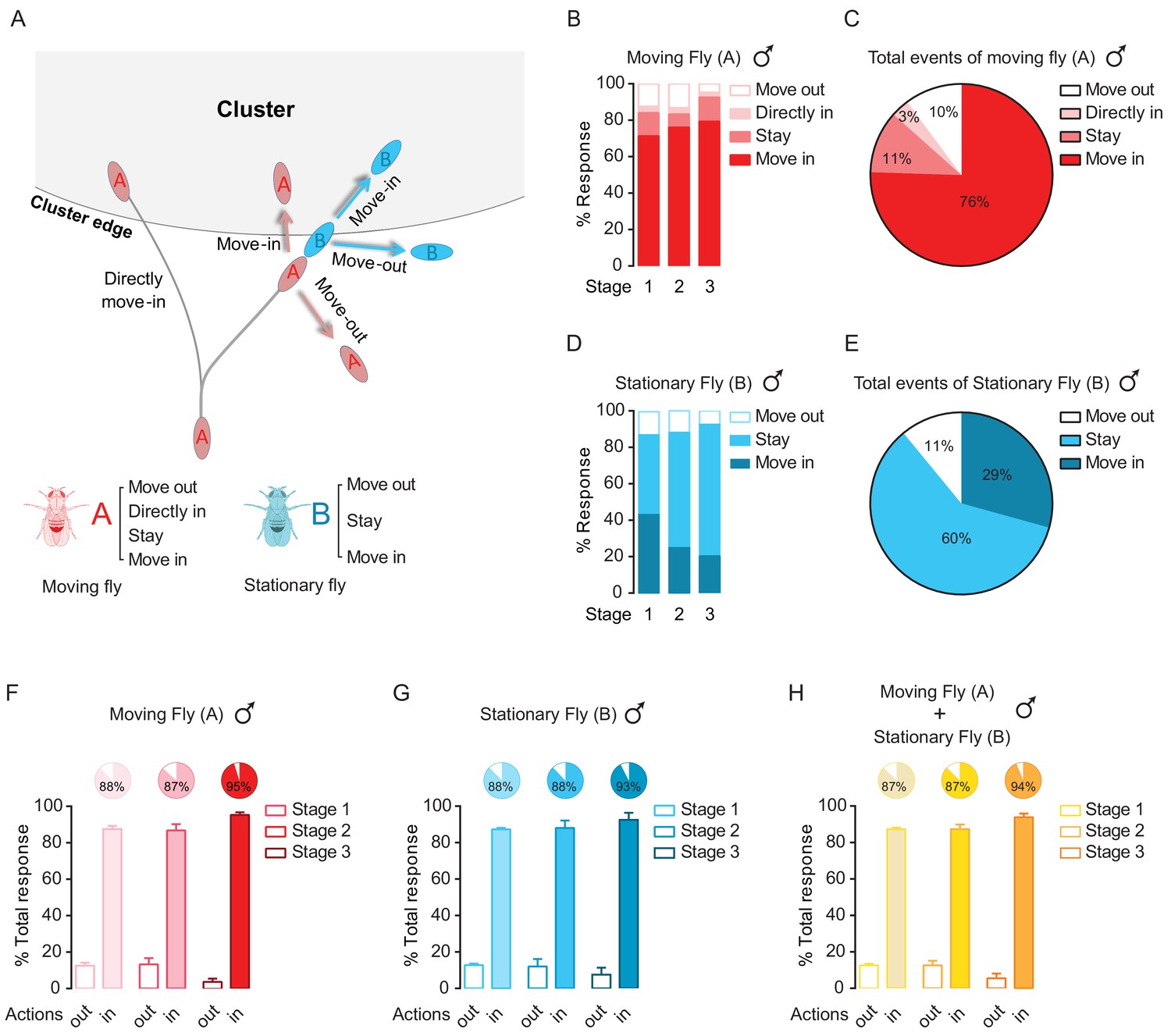
(A) A schematic showing possible events occurring near the border of a cluster. Letter ‘A’ and ‘B’ are designated as the walking fly and the stationary fly (standing at the border of a cluster), respectively. ‘Move out’: move away to leave the cluster. ‘Move in’: move to join the cluster. ‘Stay’: stay near the cluster edge. ‘Directly move in’: the walking fly joins the cluster without first interacting with any flies. (B) Percentage of different encounter outputs of male walking flies after encounters at the cluster edge at the indicated stages. (N = 4 arenas, total number of encounter events = 92). (C) Total behavioural outputs of male walking flies after encountering at the cluster edge. Data were from (B). (D) Percentage of encounter responses of male stationary flies at the cluster edge after encountering (N = 4 arenas, total number of encounter events = 92). (E) Total behavioural outputs of male stationary flies at the cluster edge after encountering. Data were from (D). (F, G) The combined percentage of joining or leaving the cluster of walking flies (F) and stationary flies (G) after encountering at the cluster edge. Data sets came from (C) and (E), respectively. ‘in’ includes ‘move in’ + ‘stay’ + ‘directly move in’, ‘out’ is ‘move out’. (H) Total percentage of behavioural output of the pairs after encountering, indicating the combined contributions by walking and stationary flies to cluster growth. Data were from (F) and (G). Values shown in (F–H) are mean ± s.e.m.
-
Figure 4—source data 1
Figure 4B, D, F, and G–H source data and related summary statistics.
- https://cdn.elifesciences.org/articles/51921/elife-51921-fig4-data1-v2.zip
Figure 4—figure supplement 1
Quantifying behavioural outputs of female encountering at the cluster edge.
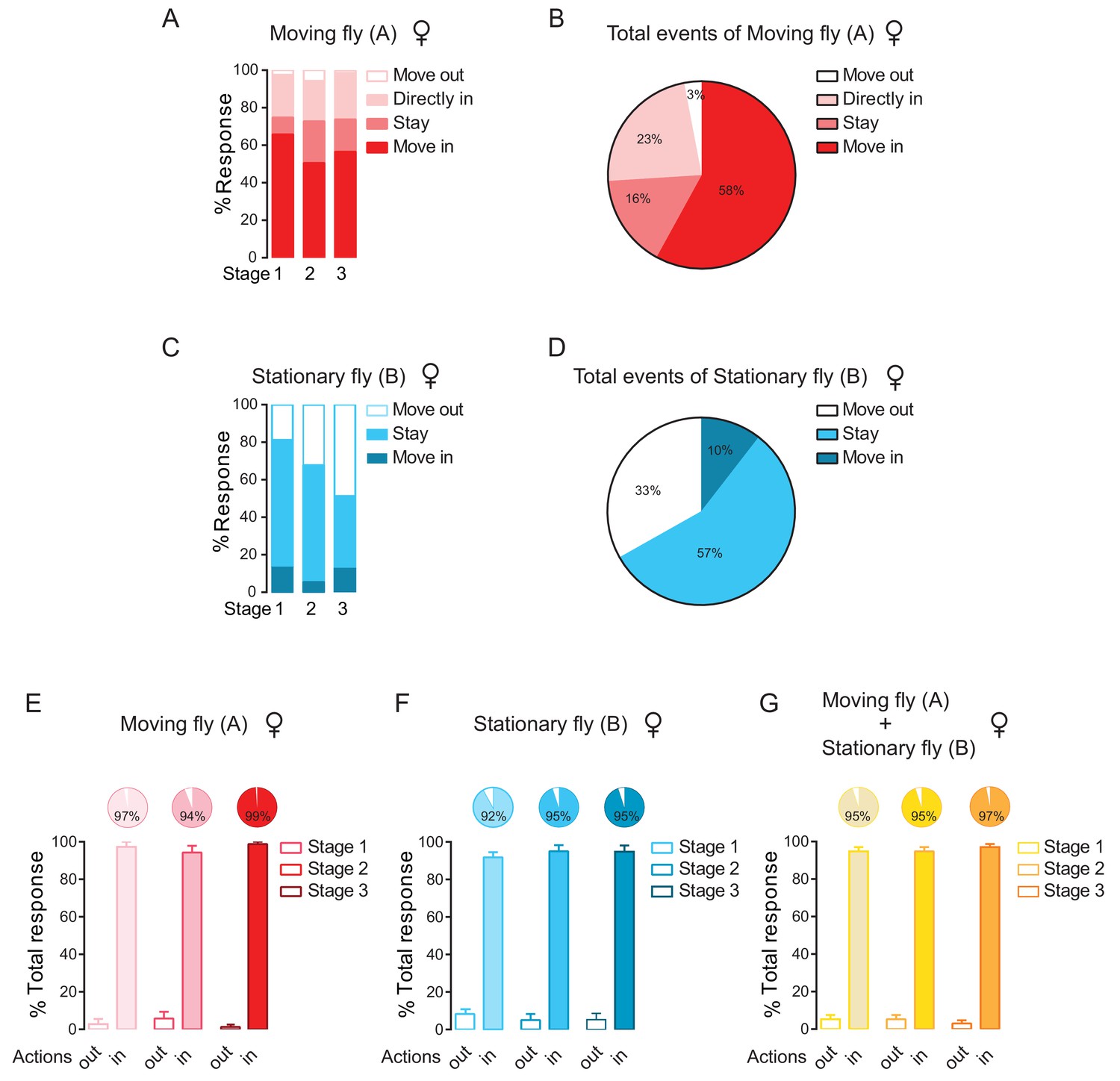
(A) Percentage of different behavioural outputs of female moving flies after encounters at the cluster edge. The outputs of the previously moving flies are: ‘Move out’ (moving away to leave the cluster), ‘Move in’ (moving in to join the cluster), ‘Stay’ (staying at the encountering site near the cluster edge), ‘Directly move in’ (walking into the cluster without first interacting with any flies at the edge). Number of encounter events = 56, number of arenas = 4. (B) Total behavioural outputs of female moving flies after encountering at the cluster edge, combining all three stages in (B). (C) Percentage of behavioural outputs of female stationary flies after encountering at the cluster edge. Number of encounter events = 56, number of arenas = 4. (D) Total behavioural outputs of female stationary flies after encountering at the cluster edge, combining all three stages in (C). (E, F) Combined percentage of joining or leaving the cluster after encountering at the cluster edge in female ‘Moving’ flies (E) and ‘stationary’ flies (F). Data sets came from (B) and (D). ‘in’ includes ‘move in’ + ‘stay’ + ‘directly move in’;‘out’ indicates ‘move out’. (H) Total percentage of behavioural output of the pairs after encountering. The values indicated the combined contributions of both moving and stationary flies to cluster growth. Data sets came from (E) and (F). Values shown in (A–G) were mean ± s.e.m.
-
Figure 4—figure supplement 1—source data 1
Figure 4—figure supplement 1A-G source data.
- https://cdn.elifesciences.org/articles/51921/elife-51921-fig4-figsupp1-data1-v2.zip
Figure 4—figure supplement 2
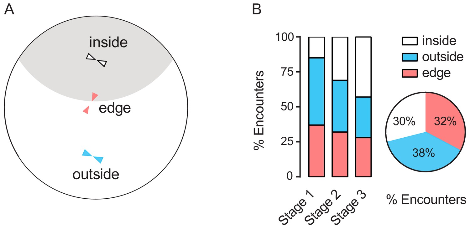
Characterising distributions of encounter events in typical regions of arena during clustering of wild-type female flies.
(A) A Schematic showing encounters occurring in three typical regions in an arena. (B) Proportions of encounter events at three typical regions during clustering stages (left) and their corresponding proportions of all observed encounter events (right) in wild-type female flies (number of arenas = 6).
-
Figure 4—figure supplement 2—source data 1
Figure 4—figure supplement 2B source data.
- https://cdn.elifesciences.org/articles/51921/elife-51921-fig4-figsupp2-data1-v2.xlsx
Figure 4—video 1
supplement to Figure 4.
A video with close-up views of pairwise interactions at the cluster edge and inside a cluster. The recording frame rate was 25 fps, sped up 2×.
Figure 5 with 1 supplement
Sensory deficits impede formation of social clusters.
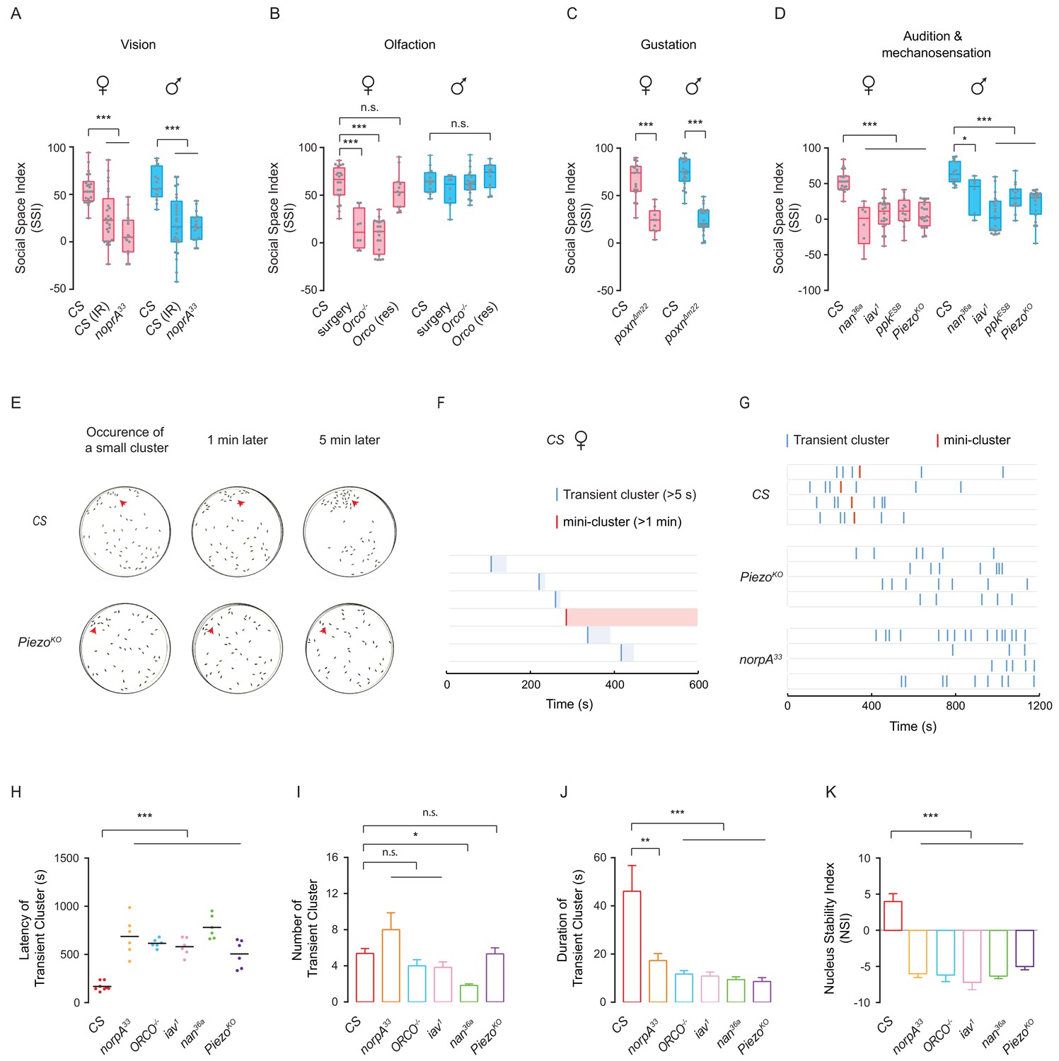
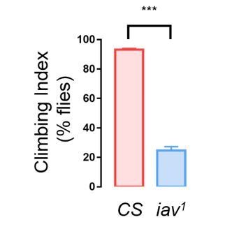
(A) The levels of SSI in flies without vision: wild-type flies under dark (illuminated by arrays of infrared LED (850 nm) and the norpA33 mutants (N = 10–25). (B) The levels of SSI of anosmic flies: wild-type flies without antennae and maxillary palps and the Orco-/- mutants (N = 8–20). (C) The levels of SSI in mutants with defective gustatory sensation (PoxnΔm22) (N = 9–26). (D) The levels of SSI in auditory/proprioceptive mutants (inactive1 and nanchung36a) and nociceptive touch mutants (ppkESB and PiezoKO) (N = 10–25). (E) Sequential images showing the spatial distribution of wild-type flies (top) and PiezoKO mutants (bottom) at 0, 1 and 5 min after the occurrence of a small cluster in each arena. Red arrows point to the sites of small clusters. (F) Representative data from an arena with the wild-type flies of indicating the onset and duration of transient clusters (blue) and mini-clusters (red). Transient clusters would be dissolved within 1 min, while a mini-cluster would last over 1 min, and served as the potential core to develop into a mature cluster. (G) Example data showing the events of transient clusters (blue) and mini-clusters (red) emergent in female CS, PiezoKO and norpA33 groups during the first 20 min of observation. Four arenas for each genotype. (H) Latency of emergence of the first transient cluster in the flies of different genotypes during 20 min (N = 6–8 arenas). (I) Number of transient clusters in flies of different genotypes during 20 min (N = 6–8 arenas). (J) Average durations of transient clusters in different genotypes during 20 min (N = 6–8 arenas). (K) Comparison of Nucleus Stability Index in flies with indicated genotypes. NSI describes the change in the size of the nascent cluster within 1 min. All genotypes and experimental conditions are indicated with the plots. In a box and whiskers plot, scatter points show all data points, the whiskers mark minimum and maximum, and the middle line indicates the median of the data set. n.s. indicates not significant (p>0.05); ***: p<0.001, **: p<0.01 (Student’s t-test within each genotype for two-group comparisons, one-way ANOVA with Dunnett’s test for multiple comparisons to control [CS]). In a bar graph plot, error bars in (H–K) indicate s.e.m.
-
Figure 5—source data 1
Figure 5A–D, H-K source data and related summary statistics.
- https://cdn.elifesciences.org/articles/51921/elife-51921-fig5-data1-v2.zip
Figure 5—figure supplement 1
Evaluating social clustering with blockage of specific sensory inputs.
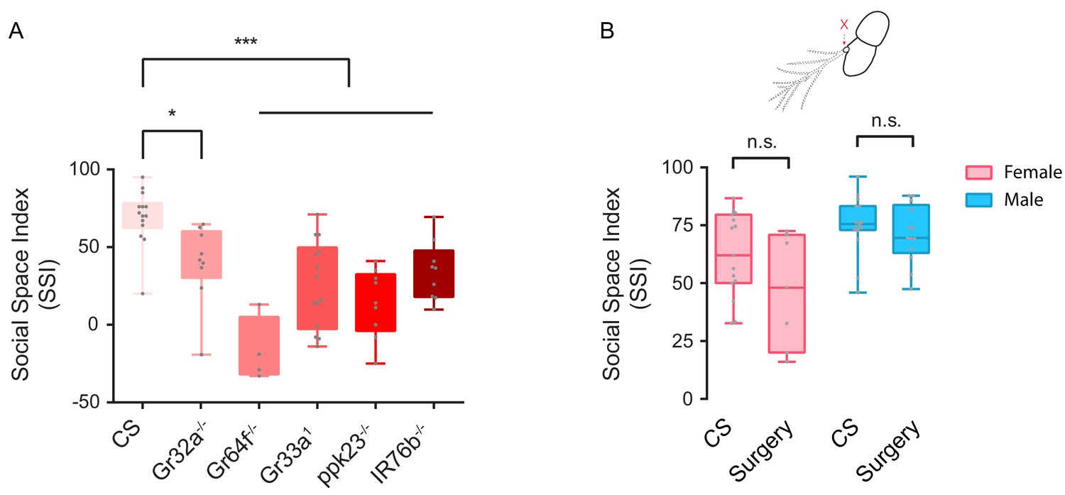
(A) SSI of female flies with defective gustatory sensation or loss of contact pheromone perception (N = 4–15). (B) SSI of wild-type female and male flies with bilateral arista surgically removed (N = 7–16). All genotypes and experimental conditions are indicated with the plots. In a box and whisker plot, scatter points show all data points, the box includes 25th to 75th percentiles, the whiskers mark the minimum and maximum, and the middle line indicates the median of the data set. Error bars indicate s.e.m. n.s. indicates not significant. * indicates p<0.05; ***: p<0.001 (Student’s t-test for two-group comparisons, one-way ANOVA followed with Dunnett’s test post hoc test for multiple comparisons).
-
Figure 5—figure supplement 1—source data 1
Figure 5—figure supplement 1A-B source data and related summary statistics.
- https://cdn.elifesciences.org/articles/51921/elife-51921-fig5-figsupp1-data1-v2.xlsx
Figure 6 with 1 supplement
Mutant flies exhibit abnormal encounter dynamics.
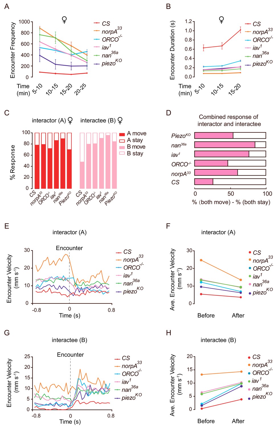
(A) Quantification of the number of encounter events during the indicated time periods in female flies of different genotypes (N = 4 arenas, n = 1090–10,205 encounters). (B) Average duration of encounters in different genotypes (60–120 encounters). The duration of an encounter is the time length from the beginning of physical contacts of two flies to the end of their last contact. (C) Percentage of behavioural outputs after encounter of the Interactor (A, red) and Interactee (B, pink), ‘A move’ and ‘B move’ indicate flies showing changes in locations after encounter, while ‘A stay’ and ‘B stay’ indicate flies that stayed at the encountering location (N = 3–5 arenas, n = 60–100 encounters). (D) Net behavioural output of the encounter events in (C). If only one fly moved away (either ‘A stay and B move’ or ‘A move and B stay’) would not change the number of flies at the encounter site since before the encounter, one fly (‘A’) walked into the site. Thus, we compared the likelihood of both A and B staying with that of both A and B moving away. The bar graph shows the difference in the percentages of these two types of outputs for each genotype (N = 3–5 arenas, n = 60–100 encounters). (E) The transient velocities of Interactors of different genotypes during the course of encounter. (N = 3 arenas, n = 30–60 encounters). (F) The average velocities of Interactors before and after encounter (N = 3 arenas, n = 30–60 encounters). (G, H) The transient velocities (G) and average velocities (H) of Interactees before and after encounter (N = 3 arenas, n = 30–60 encounters). All genotypes and experimental conditions are indicated with the plots. Error bars in (A–B) indicate s.e.m.
-
Figure 6—source data 1
Figure 6A–C, E-H source data and related summary statistics.
- https://cdn.elifesciences.org/articles/51921/elife-51921-fig6-data1-v2.zip
Figure 6—figure supplement 1
Mutants failed to form social clusters, but were capable of locomotion manoeuvers.
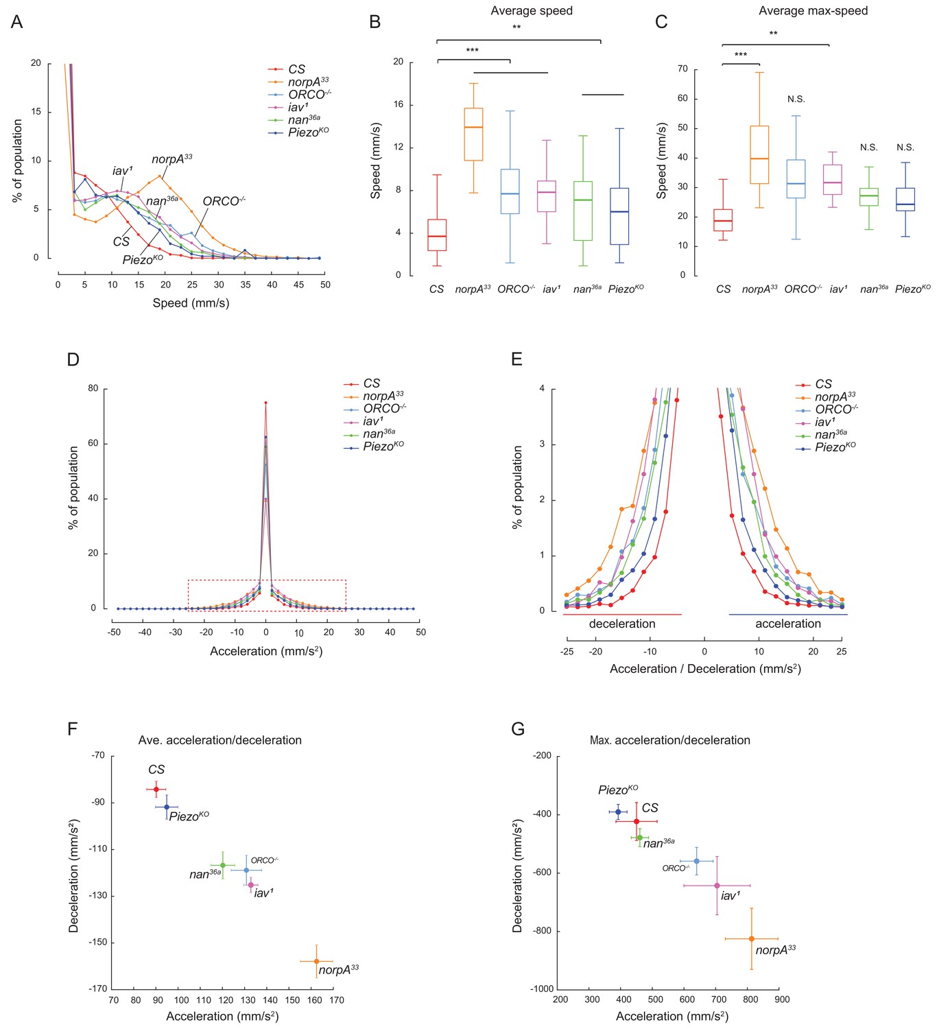
(A–C) Spontaneous locomotion activity and exploration of the flies with indicated genotypes. The speed data were obtained from short walking bouts (10 s) of individual flies 5 min after they were introduced to a dish). The duration of each step is 0.04 s. For each genotype, the number of flies were 30–60 (from 3 to 6 arenas). (A) The distribution of the walking speeds of pooled walking events of indicated genotypes. The numbers of sampled events were 7438–14,871. (B) Comparison of the average walking speed of individual flies of the indicated genotype. (C) Comparison of the maximal walking speed of individual flies of different genotypes. (D–G) Quantifying changes of speed in flies of different genotypes over a walking bout. The speed of a fly was calculated at different times, and the change of speed was then divided by the step time, 0.04 s, to obtain an acceleration/deceleration event of that fly. (D) Comparison of the distribution of pooled acceleration and deceleration events of indicated genotypes. The number of sampled events were 7406–14,790. (E) Enlarged view of (D) showing deceleration events (left half) and acceleration (right half) events. (F) Comparison of the averaged acceleration and averaged deceleration of individual flies. Data shown were mean ± s.e.m. (N = 30–60 flies). (G) Comparison of the maximal acceleration and maximal deceleration of individual flies. Data shown were mean ± s.e.m. (N = 30–60 flies). ns. indicates not significant (p>0.05); ***: p<0.001; **: p<0.01 (one-way ANOVA with Dunnett’s test for multiple comparisons to control [CS]).
-
Figure 6—figure supplement 1—source data 1
Figure 6—figure supplement 1B-C, F-G source data and related summary statistics.
- https://cdn.elifesciences.org/articles/51921/elife-51921-fig6-figsupp1-data1-v2.zip
Figure 7 with 2 supplements
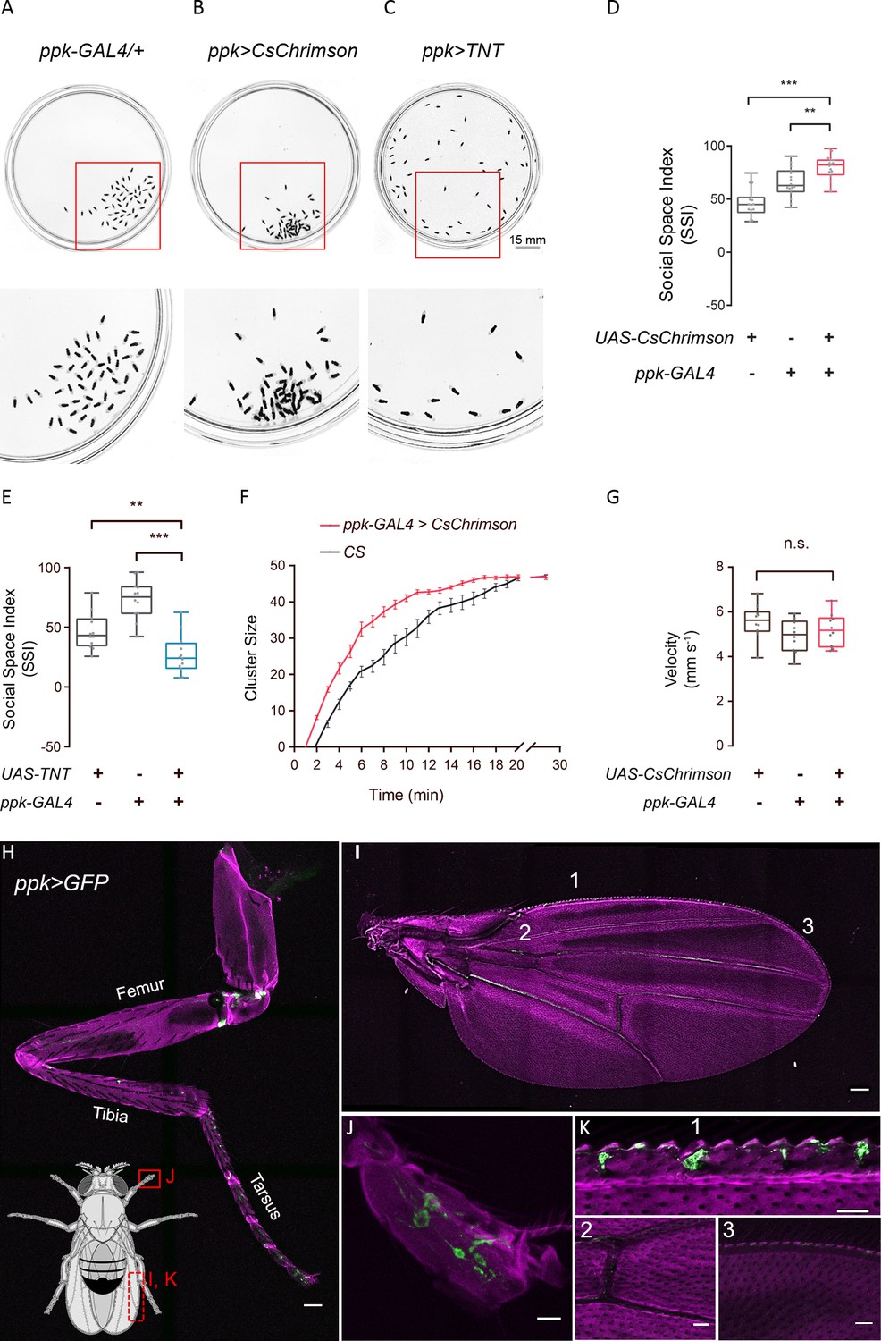
ppk-specific neurons are important for social cluster and social space.
(A–C) Representative images showing the spatial distributions of flies of genetic control (A), flies with optogenetically-activated ppk neurons (B), and flies with silenced ppk neurons (C). Bottom: the enlarged views of regions in corresponding arenas on the top, marked by red squares. (D) SSIs of flies with optogenetic activation of ppk neurons (red) and genetic controls (grey). (N = 16 arenas). (E) SSIs of flies with silenced ppk neurons (blue) and genetic controls (grey) (N = 16 arenas). (F) Comparing the cluster sizes (number of flies in a cluster) of female flies over the course of clustering (N = 8 arenas). (G) Comparing the locomotion speed in flies with optogenetically activated ppk neurons (red) and genetic controls (grey) (N = 3 arenas, n = 30 flies). (H–K) Expression pattern of ppk-GAL4 in the peripheral. Green channel shows GFP signals from ppk-GAL4 >UAS-mCD8-GFP and magenta channels show autofluorescence from the cuticle. Body parts shown are: foreleg (H, scale bar: 50 μm), wing (I, scale bar: 100 μm), tip of the tarsus (J, scale bar: 10 μm), and portions of a wing (K1: pre-wing margin, K2: vein in wing, K3: post-wing margin, scale bars in K2-3: 30 μm). All genotypes and experimental conditions are indicated with the plots. In a box and whisker plot, scatter points show all data points, the box includes the 25th to 75th percentiles, the whiskers show the minimum and maximum, and the middle line indicates the median of the data set. n.s. indicates not significant (p>0.05); **p<0.01, ***: p<0.001 (Student’s t-test). Error bars in (F) indicate s.e.m.
-
Figure 7—source data 1
Figure 7D–G source data and related summary statistics.
- https://cdn.elifesciences.org/articles/51921/elife-51921-fig7-data1-v2.zip
Figure 7—figure supplement 1
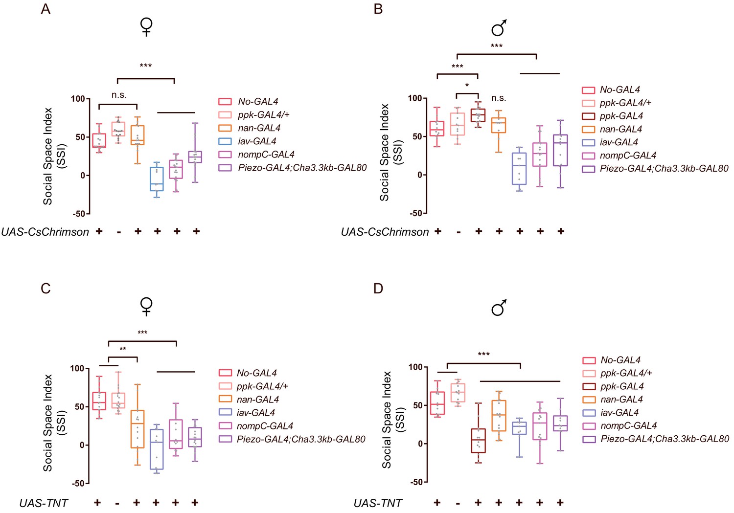
Quantification of social clustering after activating or silencing neurons related to mechanosensory function.
(A–D) Comparison of SSIs of flies with subpopulations of mechanosensory-related neurons being activated (A-B, A: females, B: males) or blocked (C-D, C: females; D: males). Different GAL4s labelled neurons involved in auditory/proprioceptive sensation (iav-GAL4 and nan-GAL4), nociceptive touch (ppk-GAL4 and Piezo-GAL4) and gentle touch (nompC-GAL4). Cha-GAL80 was used with Piezo-GAL4 to restrict Piezo neurons to legs. (N = 10–25). All genotypes are indicated with the plots. In a box and whisker plot, scatter points show all data points. The box includes 25th to 75th percentile, the whiskers mark minimum and maximum and the middle line indicates median of the data set. n.s. indicates not significant (p>0.05); * indicates p<0.05; ** indicates p<0.01; *** indicates p<0.001 (Student’s t-test).
-
Figure 7—figure supplement 1—source data 1
Figure 7—figure supplement 1A-D source data and related summary statistics.
- https://cdn.elifesciences.org/articles/51921/elife-51921-fig7-figsupp1-data1-v2.zip
Figure 7—figure supplement 2
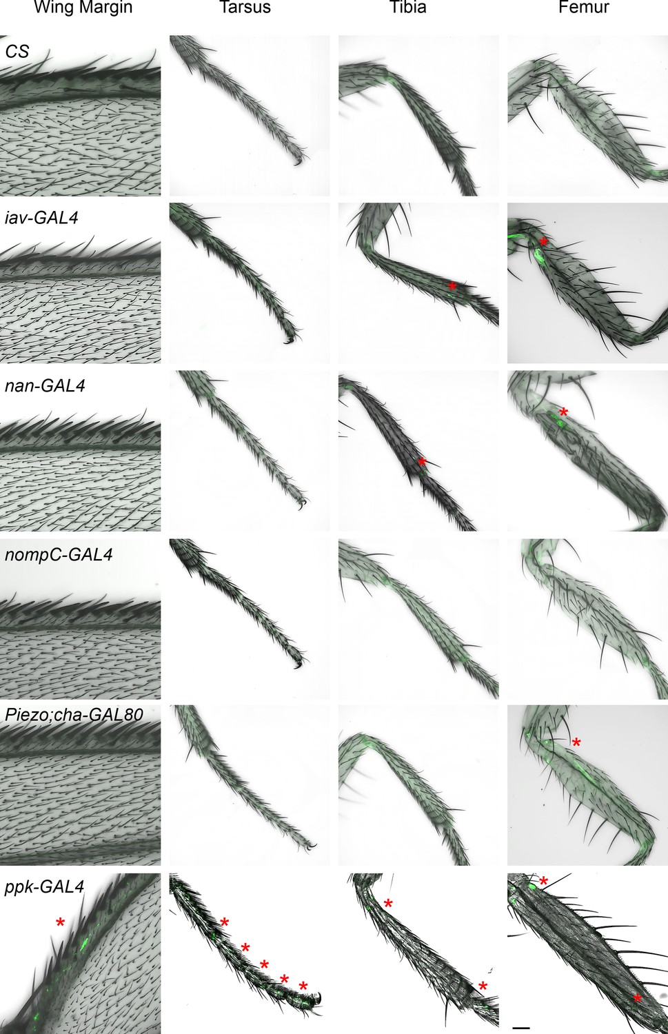
Expression patterns of mechanosensory GAL4s in the wings and legs.
GFP fluorescence signals from various Gal4s driven UAS-mCD8-GFP were superimposed on an image acquired by transmitted light. The four images of each row show the wing margin and three segments of the foreleg of flies with corresponding genotypes. Red stars indicate the GFP-positive neurons. The scale bar is 50 μm.
Figure 8 with 1 supplement
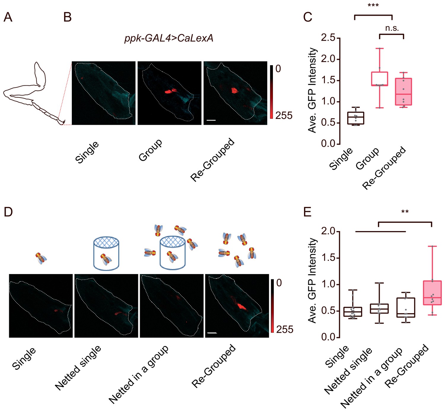
Contact-dependent activation of ppk-labelled neurons by social grouping.
(A) A schematic showing the imaging area (tip of tarsus) for (B) and (D). (B) Representative images showing CaLexA signals in ppk neurons of female flies with different social experience. Single: individual flies were raised in isolation for 16 days after eclosion; Group: flies were raised in a group for 16 days after eclosion; Re-grouped: 10 singly-raised flies were combined together and maintained for 30 hr. Cyan: autofluorescence from the cuticle, Red: maximal intensity of CaLexA signals. Dashed lines trace the tip of tarsus as ROIs for calculating GFP signals. Scale bar, 10 μm. (C) Comparing the average intensity of CaLexA signals in ppk neurons from flies treated with indicated conditions shown in (B) (N = 8 arenas). (D) Schematics of different treatments (top) and the corresponding representative images (bottom) of the tip of the tarsus of ppk-GAl4 >CaLexA flies. Single: flies raised in single isolation for 16 days after eclosion; Netted single: single fly raised in a netted tube (diameter: 12 mm, covered by double-layered net on the top end) alone for 16 d; Netted in a group: single fly raised in a netted tube which was surrounded 50 flies (inaccessible) for 16 d; Re-grouped: 10 singly-raised flies were combined and maintained for 24 hr. Cyan: autofluorescence from the cuticle, Red: maximal intensity of CaLexA signals. Dashed lines trace the tip of the tarsus (as a ROI for computing the GFP signals). Scale bar, 10 μm. (E) Comparing the average intensity of CaLexA signals in ppk neurons from flies treated with indicated conditions shown in (D) (N = 8 arenas). All genotypes and experimental conditions are indicated with the plots. In a box and whisker plot, scatter points show all data points, whiskers mark minimum and maximum, and the middle line indicates median of the data set. n.s. indicates not significant (p>0.05); **: p<0.01, ***: p<0.001 (Student’s t-test within each genotype for two-group comparisons, one-way ANOVA with Tukey’s post hoc test for multiple comparisons).
-
Figure 8—source data 1
Figure 8C, E source data and related summary statistics.
- https://cdn.elifesciences.org/articles/51921/elife-51921-fig8-data1-v2.zip
Figure 8—figure supplement 1
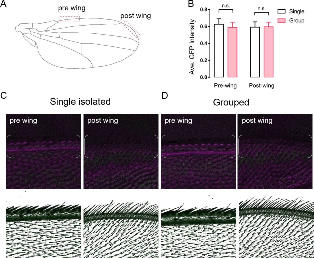
The activity of ppk-labelled neurons of wing margins under different treatments.
(A) Schematic showing the imaging areas of wing margins. The red boxes indicate the pre-wing and post-wing areas evaluated in (B–D). (B) Comparison of the CaLexA signal intensities in ppk-positive neurons of singly-raised or group-raised female flies. Single: flies were raised in isolation for 16 days; Group: flies were raised in a group of 50 flies for 16 days. (N = 8). (C, D) Representative images of wing margins in female ppk-GAL4 >CaLexA flies, raised either in isolation (C) or in a group (D). Top: magenta channel shows autofluorescence signals from cuticles, and green channel shows the maximal intensity of CaLexA signal in wing margins. White brackets indicate the areas of quantification for (B). Bottom: images of corresponding regions with the GFP channel superimposed on the channel with transmitted light. Scale bar, 10 μm. All genotypes and experimental conditions are indicated with the plots. For bar graphs, mean ± s.e.m. is shown. n.s. indicates not significant, Student’s t-test.
-
Figure 8—figure supplement 1—source data 1
Figure 8—figure supplemnet 1B source data and related summary statistics.
- https://cdn.elifesciences.org/articles/51921/elife-51921-fig8-figsupp1-data1-v2.xlsx
Author response image 1
Author response image 2
Tables
Key resources table
| Reagent type (species) or resource | Designation | Source or reference | Identifiers | Additional information |
|---|---|---|---|---|
| Strain (Drosophila melanogaster) | Canton-S | (Zhan et al., 2016) | https://doi.org/10.1038/ncomms13633 | |
| Strain (Drosophila melanogaster) | w1118 | Bloomington Drosophila Stock Center | RRID:BDSC5905 | |
| Strain (Drosophila melanogaster) | ppk-GAL4 | Bloomington Drosophila Stock Center | RRID:BDSC32079 | |
| Strain (Drosophila melanogaster) | UAS-CsChrimson | Bloomington Drosophila Stock Center | RRID:BDSC55135 | |
| Strain (Drosophila melanogaster) | Piezo-GAL4 | Bloomington Drosophila Stock Center | RRID:BDSC58771 | |
| Strain (Drosophila melanogaster) | ORCO-GAL4 | Yi Rao lab, Peking University | ||
| Strain (Drosophila melanogaster) | nan-GAL4 | Yi Rao lab, Peking University | ||
| Strain (Drosophila melanogaster) | iav-GAL4 | Yi Rao lab, Peking University | ||
| Strain (Drosophila melanogaster) | nompC-GAL4 | Yi Rao lab, Peking University | ||
| Strain (Drosophila melanogaster) | UAS-TNTE | Aike Guo and Yan Li lab (Liu et al., 2016) | http://dx.doi.org/10.7554/eLife.13238.001 | |
| Strain (Drosophila melanogaster) | Tub-GAL80ts | Aike Guo and Yan Li lab (Liu et al., 2016) | http://dx.doi.org/10.7554/eLife.13238.001 | |
| Strain (Drosophila melanogaster) | Cha3.3kb-GAL80 | Aike Guo and Yan Li lab (Zhang et al., 2013b) | https://doi.org/10.1523/JNEUROSCI.5365-12.2013 | |
| Strain (Drosophila melanogaster) | CaLexA | Jing Wang lab (Masuyama et al., 2012) | https://dx.doi.org/10.3109%2F01677063.2011.642910 | |
| Strain (Drosophila melanogaster) | UAS-mCD8::GFP | (Zhan et al., 2016) | https://doi.org/10.1038/ncomms13633 | |
| Gene (Drosophila melanogaster) | norpA33 | Bloomington Drosophila Stock Center | RRID:BDSC9047 | |
| Gene (Drosophila melanogaster) | Gr64f -/- | Bloomington Drosophila Stock Center | RRID:BDSC27883 | |
| Gene (Drosophila melanogaster) | Δppk23 | Bloomington Drosophila Stock Center | RRID:BDSC33300 | |
| Gene (Drosophila melanogaster) | Gr33a1 | Bloomington Drosophila Stock Center | RRID:BDSC31427 | |
| Gene (Drosophila melanogaster) | IR76b1 | Bloomington Drosophila Stock Center | RRID:BDSC51309 | |
| Gene (Drosophila melanogaster) | PiezoKO | Bloomington Drosophila Stock Center | RRID:BDSC58770 | |
| Gene (Drosophila melanogaster) | nan36a | Bloomington Drosophila Stock Center | RRID:BDSC24902 | |
| Gene (Drosophila melanogaster) | ORCO-/- | Yi Rao lab, Peking University | ||
| Gene (Drosophila melanogaster) | UAS-ORCO | Yi Rao lab, Peking University | ||
| Gene (Drosophila melanogaster) | iav1 | Yi Rao lab, Peking University | ||
| Gene (Drosophila melanogaster) | PoxnΔm22 | Yi Rao lab, Peking University | ||
| Gene (Drosophila melanogaster) | ppkESB | Zuoren Wang lab (Guo et al., 2014) | https://doi.org/10.1016/j.celrep.2014.10.020 | |
| Gene (Drosophila melanogaster) | ΔGr32a1 | Craig Montell lab (Moon et al., 2009) | https://doi.org/10.1016/j.cub.2009.07.061 | |
| Chemical compound, drug | Sigmacote | Sigma Aldrich | Cat #: SLBF433V | |
| Chemical compound, drug | All-trans-retinal | Sigma Aldrich | Cat #: R2500 | 200 μM |
| Software, algorithm | Prism 7 | GraphPad Prism https://www.graphpad.com/ | RRID:SCR_002798 | |
| Software, algorithm | MATLAB 2018a | MathWorks, Natick, MA https://www.mathworks.com/products/matlab.html | RRID:SCR_006752 | |
| Software, algorithm | Fiji | NIH https://fiji.sc/ | RRID:SCR_002285 | |
| Software, algorithm | Adobe Illustrator | Adobe https://www.adobe.com/ | RRID:SCR_010279 | |
| Software, algorithm | Adobe Premiere pro | Adobe https://www.adobe.com/ | ||
| Code | Simulation of random flies/dots | This paper | Materials and methods | |
| Other | White LED/Infrared LED arrays (850 nm) | Xin Xing Yuan Guangdian https://item.taobao.com/item.htmid=20158878058 |
Additional files
-
Source code 1
randomdot_simfunc.
- https://cdn.elifesciences.org/articles/51921/elife-51921-code1-v2.m
-
Source code 2
randomfly_from_dataset.
- https://cdn.elifesciences.org/articles/51921/elife-51921-code2-v2.m
-
Transparent reporting form
- https://cdn.elifesciences.org/articles/51921/elife-51921-transrepform-v2.pdf
Download links
A two-part list of links to download the article, or parts of the article, in various formats.
Downloads (link to download the article as PDF)
Open citations (links to open the citations from this article in various online reference manager services)
Cite this article (links to download the citations from this article in formats compatible with various reference manager tools)
Emergence of social cluster by collective pairwise encounters in Drosophila
eLife 9:e51921.
https://doi.org/10.7554/eLife.51921


