Distinct cytoskeletal proteins define zones of enhanced cell wall synthesis in Helicobacter pylori
- University of Washington, United States
- Fred Hutchinson Cancer Research Center, United States
- Princeton University, United States
- University of Delaware, United States
- Harvard Medical School, United States
- Newcastle University, United Kingdom
- Indiana University, United States
Figures
Figure 1

Helical cell surfaces feature areas of distinct curvatures.
(A) 3D SIM images of individual H. pylori cells stained with fluorescent wheat germ agglutinin (WGA). Top-down view (left) and 90-degree rotation about the long axis (right). Scale bar = 0.5 µm; images from one experiment. (B) Corresponding views of computational surface reconstructions of cells in (A). with Gaussian curvature plotted (scale at right - blue: moderate negative; white: zero; red: moderate positive; gray: high positive). Computationally-defined polar regions are delineated by the thin black line. Polar regions correspond to regions whose centerline points are within 0.75 of a cell diameter to the terminal pole positions. (C) Schematic of minor (blue line) and major (red line) helical axes.
Figure 2
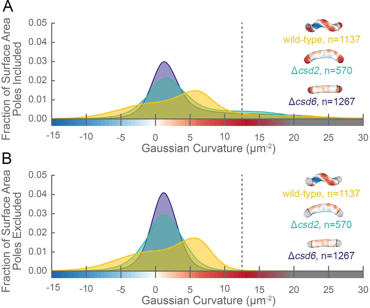
The distribution of surface Gaussian curvature for helical cells is distinct from that of curved- and straight-rod cells.
Smooth histograms of the distribution of surface Gaussian curvatures for a population of cells (wild-type helical, yellow; curved-rod Δcsd2, teal; straight-rod Δcsd6, indigo) with poles included (A) or sidewall only (B, poles excluded). The region to the right of the dotted vertical lines corresponds to curvatures contributed almost exclusively by the poles. Histograms are derived using a bin size of 0.2 µm−2. Example computational surface reconstructions (top right of each histogram) of a wild-type helical, curved-rod Δcsd2, and straight-rod Δcsd6 cell with Gaussian curvatures displayed as in Figure 1. The data represented are from one replicate.
Figure 3 with 4 supplements

Three-dimensional shape properties of a wild-type helical population.
Analysis of the wild-type population in Figure 2 from the 231 wild-type cells for which the cell centerline was well-fit by a helix. (A) Schematic of helical-rod shape parameters (cell centerline length, gray; cell diameter, purple; helical pitch, pink; and helical diameter, green). (B) Example cell with helical coordinate system and the major (red line, 0°) and minor (blue line, 180°) helical axes shown on the cell sidewall. Population distributions of (C) cell centerline lengths, (D) average cell diameters, (E) helical pitch, (F) helical diameter, (G) major to minor axis length ratio, and (H) the average Gaussian curvature for a given helical coordinate system unwrap angle. Colored dotted lines in (C–G) indicate the mean ±1.5 standard deviations in 0.5 standard deviation steps. Shaded line in (H) indicates ±1 standard deviation about the mean. Distributions of parameters (C–D) are from real cells, parameters (E–F) are from helical centerline fits, and properties (G–H) are measured from the matched synthetic cell sidewalls.
Figure 3—figure supplement 1
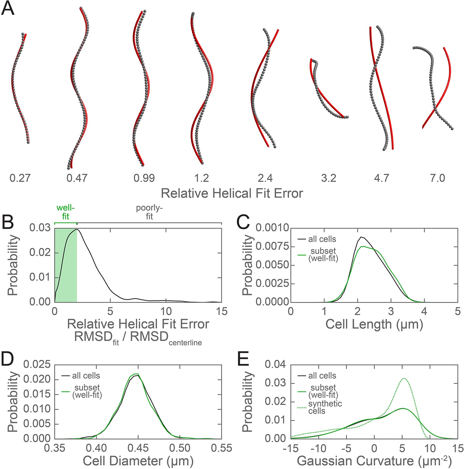
Evaluation of the subset of the wild-type population used to generate synthetic cells.
(A) Example cell centerlines (gray dots) and calculated helical fits (red lines), arranged from good (left) to poor (right) fit. (B) Histogram of the relative helical fit error for each of the cells from the wild-type population shown in Figure 2. Shaded green box indicates well-fit centerlines with a relative helical fit error below the selected threshold of 2, which were used for further analysis. Comparison of the population distribution of (C) cell lengths and (D) average cell diameters for the entire wild-type population (black line) and the subset of cells with a centerline that was well fit by a helix (green). (E) Comparison of the population cell surface Gaussian curvature distribution for the entire wild-type population (black line), the selected subset of wild-type cells (green line), and the synthetic cells generated based on the cell centerline helical fits of the selected subset (dotted green line).
Figure 3—figure supplement 2
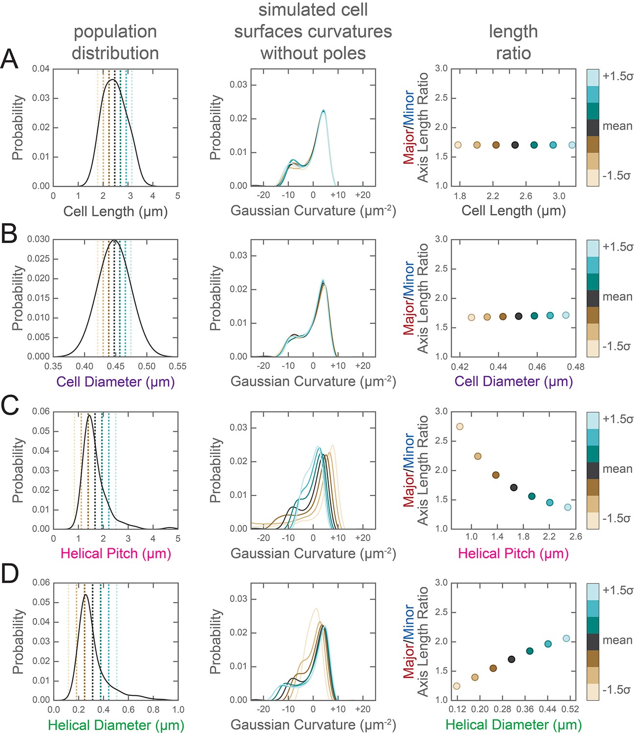
Change in the distribution of cell surface Gaussian curvatures based on modulating helical rod parameters.
Left column, distribution of population helical rod parameters from Figure 3C–F. Center column, Gaussian surface curvature distribution of the synthetic cells in (Figure 3—figure supplement 3) without poles for (A) cell centerline length, (B) cell diameter, (C) helical pitch, and (D) helical radius modulated to the mean ±1.5 standard deviations in 0.5 standard deviation increments. Right column, ratio of major to minor axis length vs. (A) cell centerline length, (B) cell diameter, (C) helical pitch, and (D) helical radius modulated to the mean ±1.5 standard deviations in 0.5 standard deviation increments. As shown in the color bar at the far right, data for the mean cell data are plotted in gray; data for cells generated with a parameter modulated to a value greater than the mean are shown in blue tones; and data for cells generated with a parameter modulated to a value less than the mean are shown in tan tones.
Figure 3—figure supplement 3
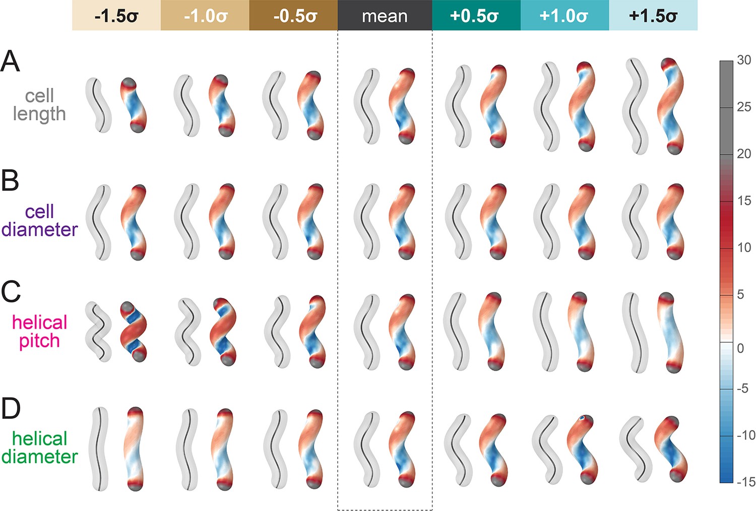
Simulated helical cells demonstrating how variation in helical parameters alters surface Gaussian curvature.
Cell centerline (paired cells, left) and cell surface Gaussian curvatures (paired cells, right) of synthetic, idealized cells with parameters taken from the distribution of wild-type shapes. The central pair of cells in each row was generated using the average value for each shape parameter shown in Figure 3 and is the same for all rows. Each of the parameters (A) cell centerline length, (B) cell diameter, (C) helical pitch, and (D) helical radius is increased (right of mean cell pair) and decreased (left of mean cell pair) up to 1.5 standard deviations in 0.5 standard deviation increments while leaving the remaining three parameters fixed at the population mean.
Figure 3—video 1
Rotation of example cell centerlines (gray dots) and calculated helical fits (red lines), arranged from good (left) to poor (right) fit from Figure 3—figure supplement 1A.
Figure 4 with 4 supplements

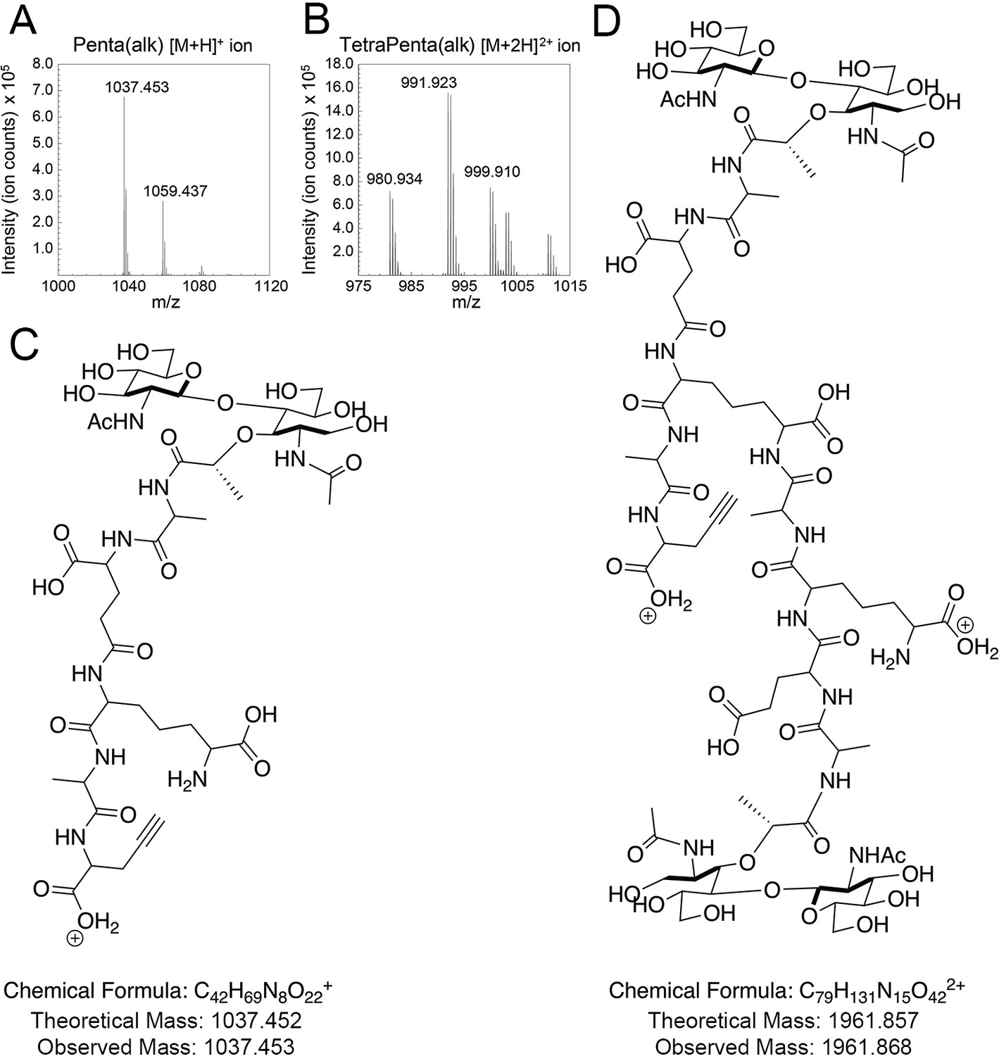
Validation of PG metabolic probes.
(A) 10-fold dilutions showing LSH108 (rdxA::catsacB) or HJH1 (rdxA::amgKmurU) treated with 50 µg/ml fosfomycin or untreated and with or without 4 mg/ml MurNAc supplementation, from one representative of three biological replicates. (B and C) Verification of MurNAc-alk incorporation into pentapeptides (left column) and tetra-pentapeptides (right column) by HPLC/MS/MS. (B) Extracted ion chromatograms (EICs) for the ion masses over the HPLC elution for unlabeled (lower EIC) and labeled (top EIC) sacculi. (C) Spectra of the ions observed during LC-MS for the MurNAc-alk pentapeptide (left, non-reduced, predicted [M+H]+ ion m/z = 1049.452) and MurNAc-alk tetra-pentapeptide dimer (right, non-reduced, predicted [M+2H]2+ ion m/z = 985.920). (D) Verification of D-Ala-alk incorporation into pentapeptides and tetra-pentapeptides. HPLC chromatograms of labeled (top) and unlabeled (bottom) sacculi. The main monomeric and dimeric muropeptides are labeled (4, disaccharide tetrapeptide; 5, disaccharide pentapeptide; 44, bis-disacccharide tetratetrapeptide; 45, bis-disacharide tetrapentapeptide). D-Ala-alk-modified muropeptides (top, 5a and 45a) are present only in the sample from labeled cells and were confirmed by MS analysis of the collected peak fractions. 5a, alk-labeled disaccharide pentapeptide (neutral mass: 1036.448); 45a, alk-labelled bis-disaccharide tetrapentapeptide (neutral mass: 1959.852). Data (B, C, and D) are from one replicate.
Figure 4—figure supplement 1
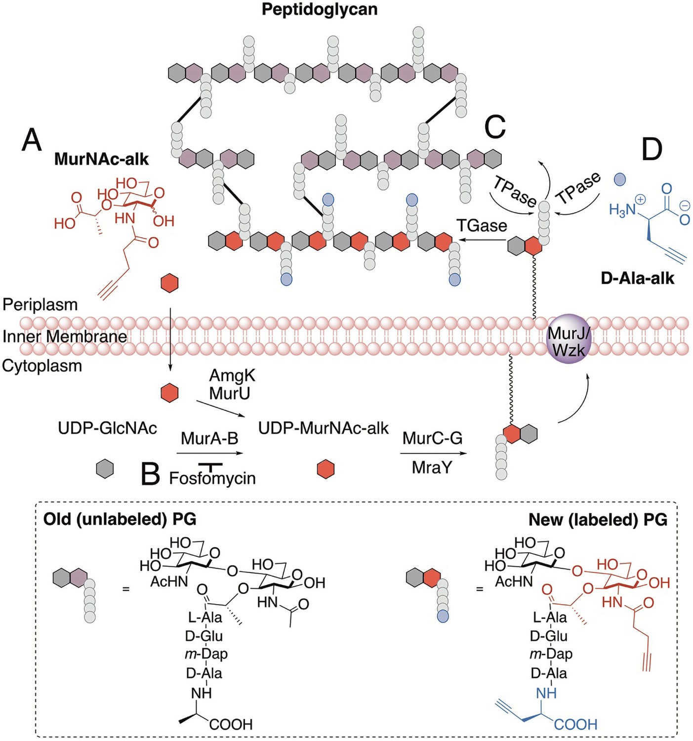
Schematic of PG synthesis and incorporation of PG metabolic probes.
(A) MurNAc-alk diffuses across the cell membrane and is converted into UDP-MurNAc-alk, which can then be used in the synthesis of PG precursors. (B) Fosfomycin inhibits the conversion of UDP-GlcNAc to UDP-MurNAc. Addition of exogenous MurNAc allows the cell to bypass this step and survive when treated with fosfomycin. To incorporate the new PG monomer into the cell wall, transglycosylases (TGase) polymerize the glycan strand. (C) To link the new strand to the existing PG, transpeptidases (TPase) form a crosslink between the tetra position D-Ala of the new peptide stem and the m-Dap of a nearby peptide stem, resulting in loss of the penta position D-Ala from the new peptide stem. (D) In a reaction similar to forming a crosslink, TPases can replace the penta position D-Ala with D-Ala-alk. In our experiments labeling PG incorporation, we labeled cells with either MurNAc-alk or D-Ala-alk.
Figure 4—figure supplement 2
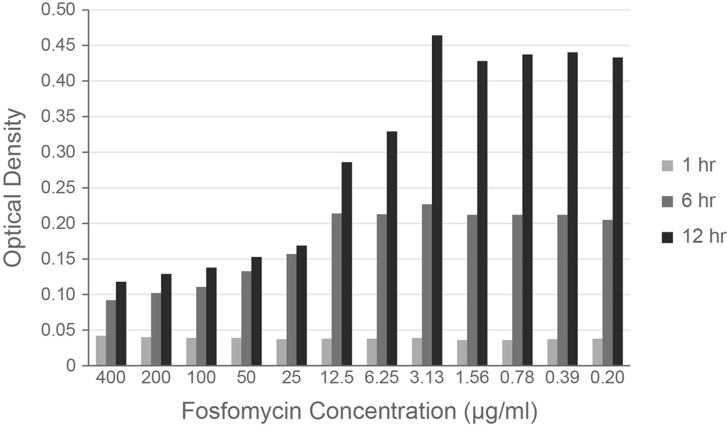
The MIC of fosfomycin in H. pylori is 25 µg/ml.
Optical density of wild-type H. pylori cultures grown in a 96-well plate with a 2-fold dilution series of fosfomycin. Optical density was measured at 1 (light gray), 6 (medium gray), and 12 (dark gray) hours of incubation. Figure shows one representative of two biological replicates.
Figure 4—figure supplement 3
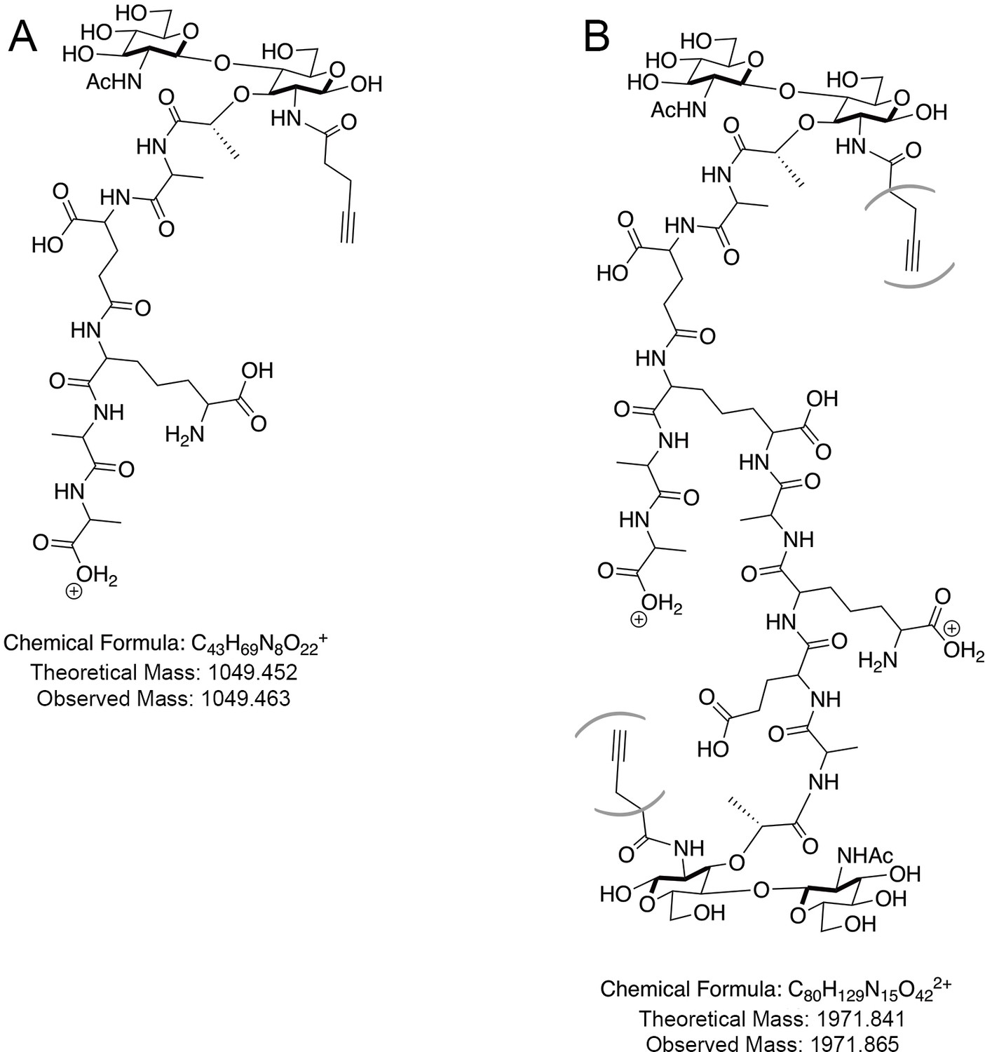
Detected MurNAc-alk labeled muropeptides.
Labeled (A) pentapeptide monomer and (B) tetra-pentapeptide dimer ions. Parentheses indicate that the MurNAc-alk could be on either the tetra or penta portion of the dimer; these two species are indistinguishable in our HPLC/MS/MS data.
Figure 4—figure supplement 4
Detected D-Ala-alk labeled muropeptides.
Mass spectra for the ions observed for the reduced (A) D-Ala-alk pentapeptides (left, Peak 5a in Figure 4D) and (B) D-Ala-alk tetra-pentapeptides (right, Peak 45a in Figure 4C). The labeled peaks, from left to right are: (A) D-Ala-alk-pentapeptide+H+ and D-Ala-alk-pentapeptide+Na+ and (B) D-Ala-alk-tetra-pentapeptide+2 H2+, D-Ala-alk-tetra-pentapeptide+H++Na+, and D-Ala-alk-tetra-pentapeptide+H++K+. Schematic of (C) labeled pentapeptide monomer and (D) labeled tetra-pentapeptide dimer ions.
Figure 5 with 1 supplement

New cell wall growth appears dispersed along the sidewall, excluded from poles, and present at septa.
3D SIM imaging of wild-type cells labeled with an 18 min pulse of MurNAc-alk (A–D, yellow) or 18 min pulse of D-Ala-alk (E–H, yellow) counterstained with fluorescent WGA (blue). Color merged maximum projection of 18 min MurNAc-alk (A), D-Ala-alk (E), or mock (B, F) labeling with fluorescent WGA counterstain. (C, G) Top-down (left) and 90-degree rotation (right) 3D views of three individual cells, including a dividing cell at the right. Top: color merge; middle: 18 min MurNAc-alk (C) or D-Ala-alk (G); bottom: fluorescent WGA. (D, H) Color merged z-stack views of the three cells in (C, G), respectively (left to right = top to bottom of the cell). Numbering indicates matching cells. Scale bar = 0.5 µm. The representative images are selected from one of three biological replicates.
Figure 5—video 1
Volumetric rendering and z-slices of the example cells in Figure 5.
Figure 6 with 2 supplements
New cell wall growth is excluded from the poles and enriched at negative Gaussian curvature and the major axis area.
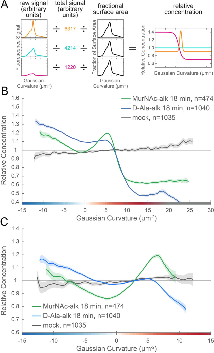
(A) The calculation of relative concentration for a specific probe involves two steps of normalization. First, the raw signal is summed up in bins defined by the Gaussian curvature at the surface. Then, this raw signal is normalized by dividing by the sum of the raw signal at all Gaussian curvatures (total signal). This normalizes for changes in total signal, fluorophore brightness, imaging conditions, etc. The second step is to divide by the fractional surface area, or amount of surface area contributed by each Gaussian curvature bin. This distribution is dependent on the observed shape of the cell. Following these two normalization steps, one has the concentration of the probe of interest relative to a uniformly distributed null model. For illustration, we have shown this graphical equation for three noise-free cells that have the same geometry, but different relative signal abundances. In the experimental data presented in the main text, the single cell relative concentration profile is averaged over hundreds of cells, each with their own unique geometry. Whole surface (B) and sidewall only (C) surface Gaussian curvature enrichment of relative concentration of new cell wall growth (y-axis) vs. Gaussian curvature (x-axis) derived from a population of computational cell surface reconstructions of MurNAc-alk (green), D-Ala-alk (blue) 18 min pulse-labeled, and mock-labeled (gray) cells. 90% bootstrap confidence intervals are displayed as a shaded region about each line. The represented data are pooled from three biological replicates.
Figure 6—figure supplement 1
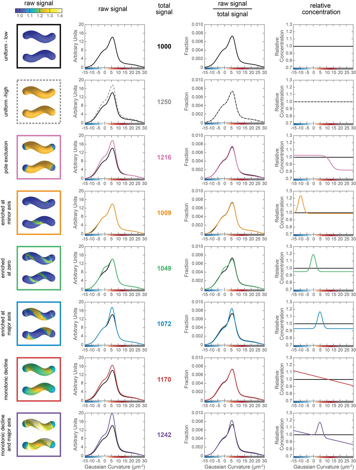
For eight different example distributions (rows with brief labels to the left), five pieces of data are shown.
The five columns are as follows (from left to right): two views of an example rendering of a helical rod cell colored by the intensity of the raw signal at each point on the surface; the raw signal summed across all surface elements of the same curvature; the total raw signal summed across all curvature values; the ratio of the raw signal to total signal; and the relative concentration. For plots that are functions of Gaussian curvature, the solid black line from the ‘uniform – low’ example is included in all plots for comparison. The same idealized cell geometry was used for all the examples. The simulated example distributions were created by taking a uniformly distributed signal and adding 25% additional signal to specific geometries. This additional signal results in the raw signal being 1.25X larger at the enriched geometries than the uniform case. However, the increase in the total signal is geometry dependent and not 25%, except in the ‘uniform – high' example. Because of the normalization steps, an identical relative concentration profile could have been generated by removing material from the opposite regions.
Figure 6—figure supplement 2
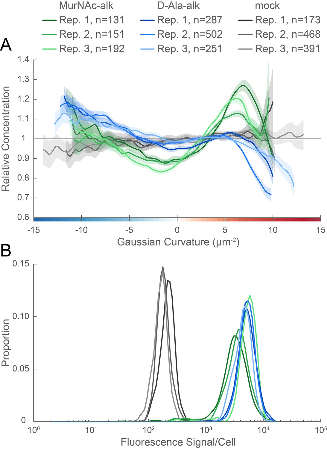
Curvature enrichment analysis of biological replicates of MurNAc-alk-, D-Ala-alk-, and mock-labeling.
(A) Sidewall only surface Gaussian curvature enrichment of relative concentration of new cell wall growth (y-axis) vs. Gaussian curvature (x-axis) of the three biological replicates pooled in Figure 6: MurNAc-alk (greens), D-Ala-alk (blues) 18 min pulse-labeled, and mock-labeled (grays) cells. 90% bootstrap confidence intervals are displayed as a shaded region about each line. (B) Histogram of fluorescence signal per cell divided by the number of pixels in the projected cell area for the populations in (A).
Figure 7 with 4 supplements
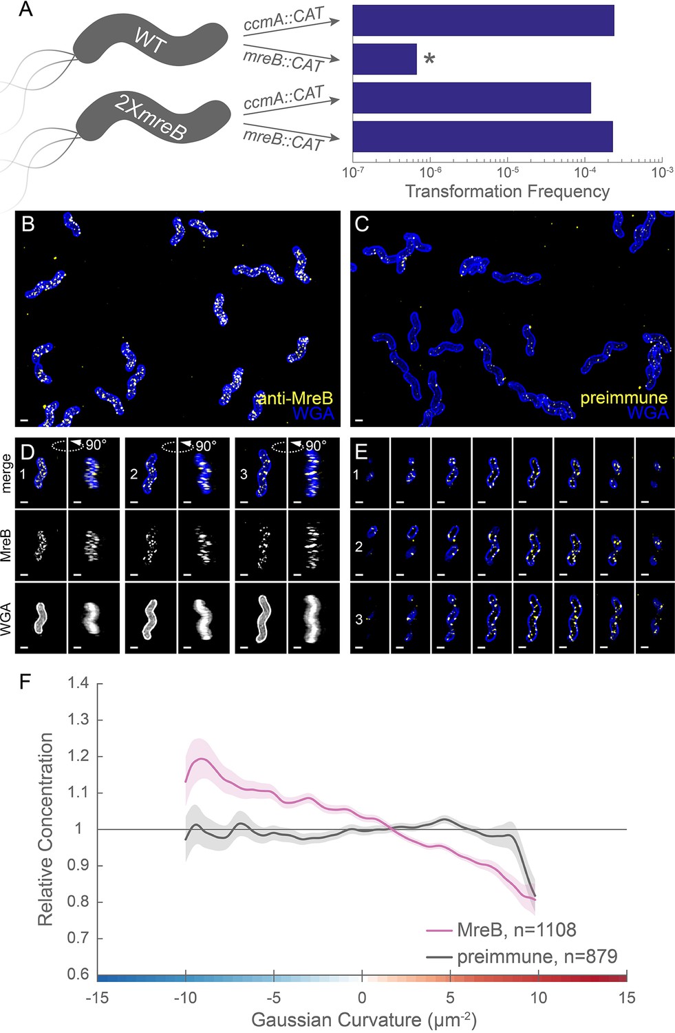
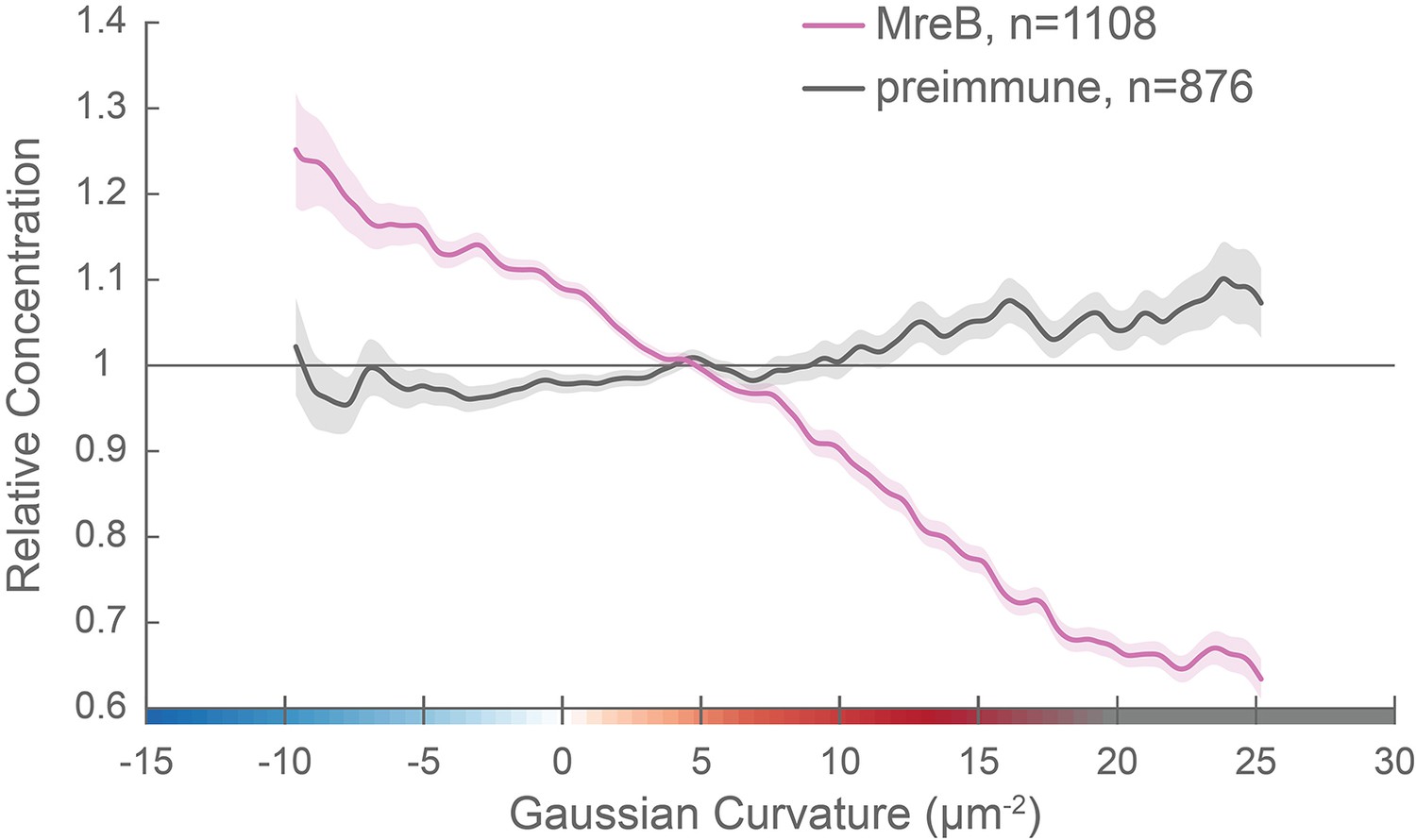
MreB is essential in LSH100 and is present as small foci enriched at negative Gaussian curvature.
(A) Schematic of transformation experiment testing MreB essentiality in LSH100 (WT) and IM4 (2XmreB) (left) and corresponding transformation frequencies (right). *=two recombinant clones with mreB duplication (see Figure 7—figure supplement 1 for details). 3D SIM imaging of wild-type cells immunostained with anti-MreB (B, D, E, yellow) or preimmune serum (C, yellow) and counterstained with fluorescent WGA (blue). (B, C) Color merged maximum projections (D) Top-down (left) and 90-degree rotation (right) 3D views of three individual cells. Top: color merge; middle: anti-MreB; bottom: fluorescent WGA. (E) Color merged z-stack views of the three cells in (A). (left to right = top to bottom of the cell). Numbering indicates matching cells. Scale bar = 0.5 µm. (F) Sidewall only surface Gaussian curvature enrichment plots for a population of cells immunostained with anti-MreB (pink), or preimmune serum (gray). Smooth line plot (solid line) of relative MreB concentration (y-axis) vs. Gaussian curvature (x-axis) derived from a population of computational cell surface reconstructions with poles excluded. 90% bootstrap confidence intervals are displayed as a shaded region about each line. The representative images are selected from one of three biological replicates and the data shown in (F) are pooled from the three biological replicates.
Figure 7—figure supplement 1
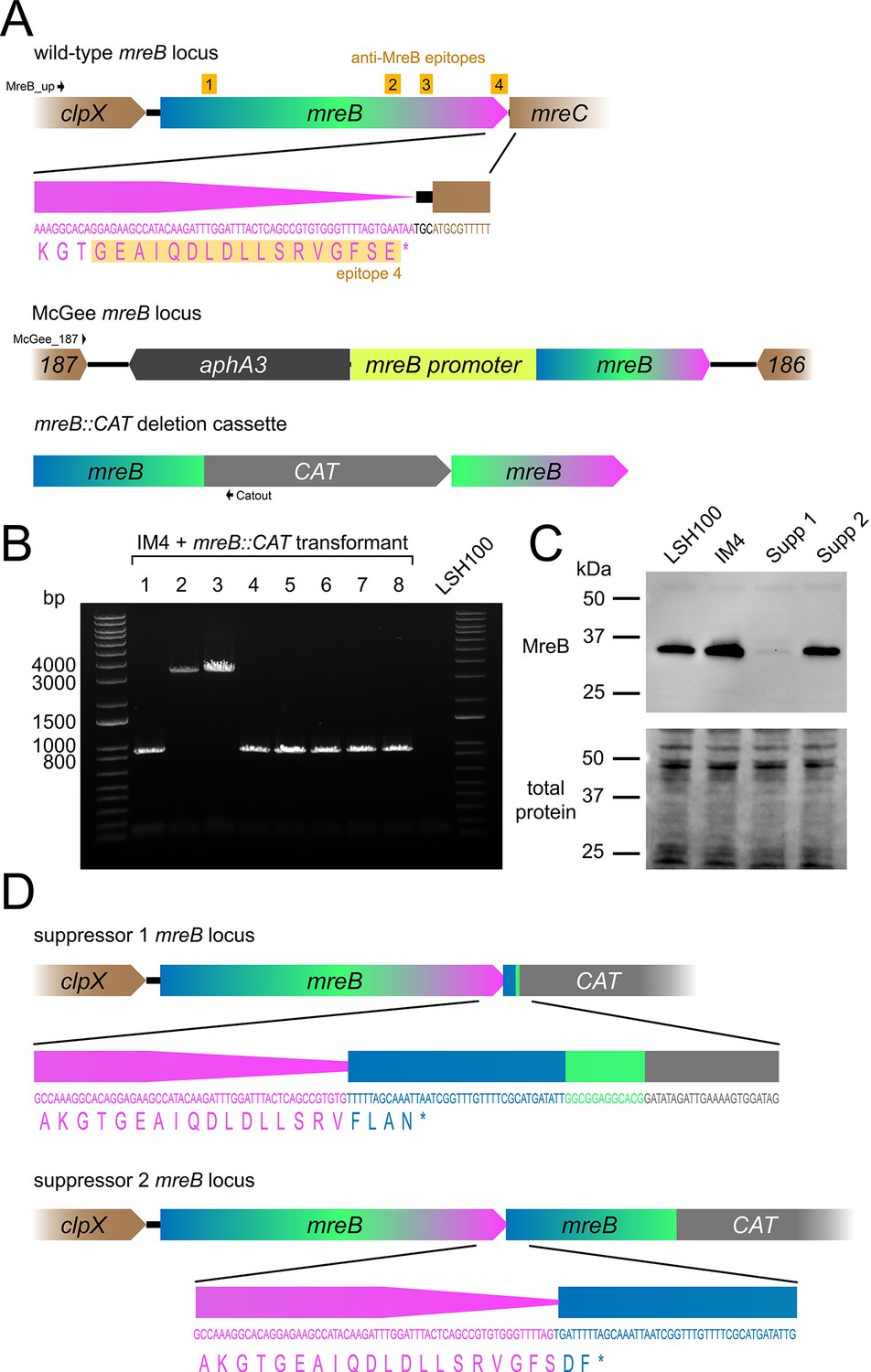
MreB is essential in the G27 derivative LSH100.
(A) (Top) Schematic of the LSH100 native mreB locus with DNA and protein sequence for a small region at the C-terminus. Anti-MreB epitopes are annotated in yellow. (Middle) Schematic of the McGee locus with mreB in strain IM4. (Bottom) mreB::CAT deletion cassette used for transformations. Black arrows: primers MreB_up, McGee_187, and Catout used for CAT insertion site characterization in (B). (B) PCR to determine the integration site of mreB::CAT into IM4. Native locus expected size = 899 bp; McGee locus expected size = 3320 bp. (C) Western blot of MreB expression (top) and total protein levels (bottom) in LSH100 (wild-type), IM4 (2XmreB), and mreB recombinant clone #1 and #2. One of two representative experiments. (D) Schematic of the mreB duplications in MreB suppressor clone #1 (top) and #2 (bottom) with DNA and protein sequence for a small region at the C-terminus. Schematics are to scale; McGee mreB locus schematic is presented at ½ scale.
Figure 7—figure supplement 2
MreB enrichment decreases with increasing positive Gaussian curvature.
Whole surface (sidewall and poles) Gaussian curvature enrichment of relative MreB concentration (y-axis) vs. Gaussian curvature (x-axis) of computational cell surface reconstructions of a population of cells immunostained with anti-MreB (pink), or preimmune serum (gray). 90% bootstrap confidence intervals are displayed as a shaded region about each line. The represented data are pooled from three biological replicates.
Figure 7—figure supplement 3
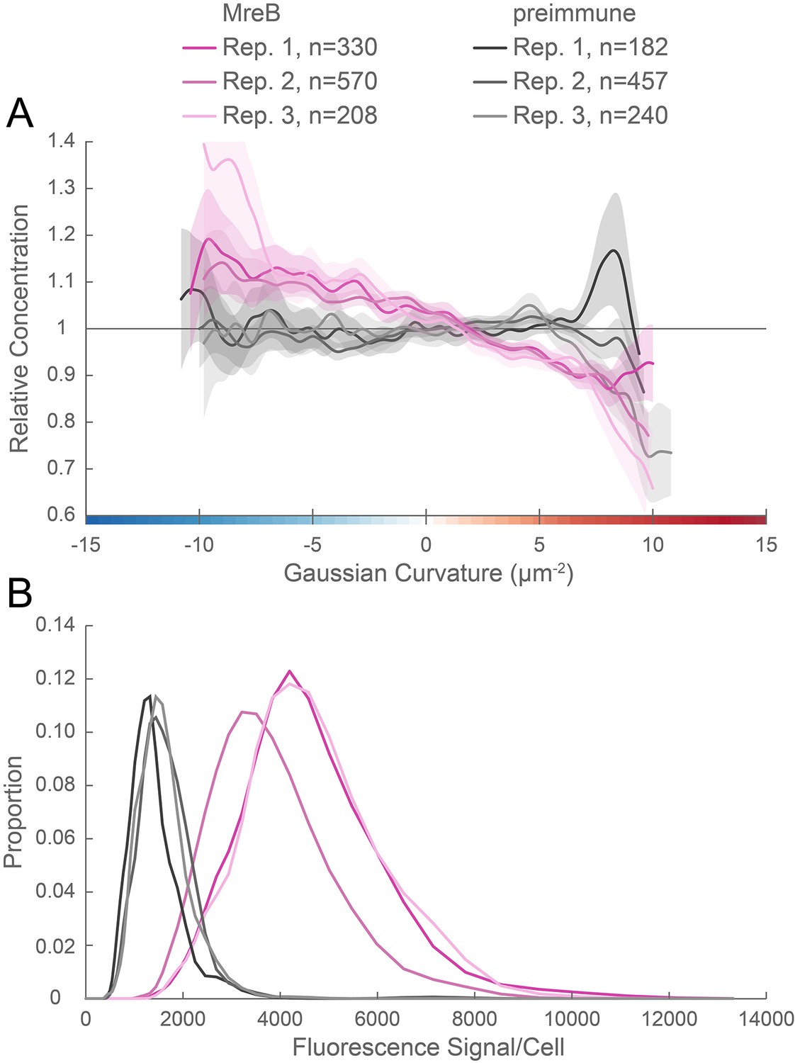
Curvature enrichment analysis of biological replicates of MreB.
(A) Sidewall only surface Gaussian curvature enrichment of relative MreB concentration (y-axis) vs. Gaussian curvature (x-axis) of the three biological replicates pooled in Figure 7: anti-MreB (pinks) and preimmune serum (grays) immunostained cells. 90% bootstrap confidence intervals are displayed as a shaded region about each line. (B) Histogram of fluorescence signal per cell divided by the number of pixels in the projected cell area for the populations in (A).
Figure 7—video 1
Volumetric rendering and z-slices of the example cells in Figure 7.
Figure 8 with 2 supplements
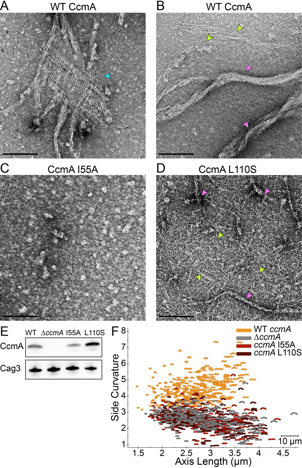
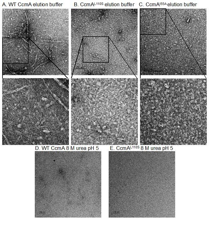
Amino acid substitution mutations in CcmA cause altered polymerization in vitro and alter cell shape in vivo.
(A–D) Negatively stained TEM images of purified CcmA. Scale bars = 100 nm, with representative images from one of three biological replicates. Wild-type CcmA lattices (A) (blue arrows) and helical bundles (B) (pink arrows), which are comprised of individual filaments (lime green arrows). (C) The I55A variant does not form ordered structures in vitro. (D) CcmAL110S filament bundles (pink arrows) and individual filaments (lime green arrows). (E) Immunoblot detection of CcmA expression (top) in H. pylori lysates using Cag3 as loading control (bottom); representative of four experiments. (F) Scatterplot displaying axis length (x-axis) and side curvature (y-axis) of wild-type (gold), ∆ccmA (gray), ccmAI55A (red), and ccmAL110S (dark red) strains. Data are representative of two biological replicates. Wild-type, n = 346; ∆ccmA, n = 279; ccmAI55A, n = 328; and ccmAL110S, n = 303.
Figure 8—figure supplement 1
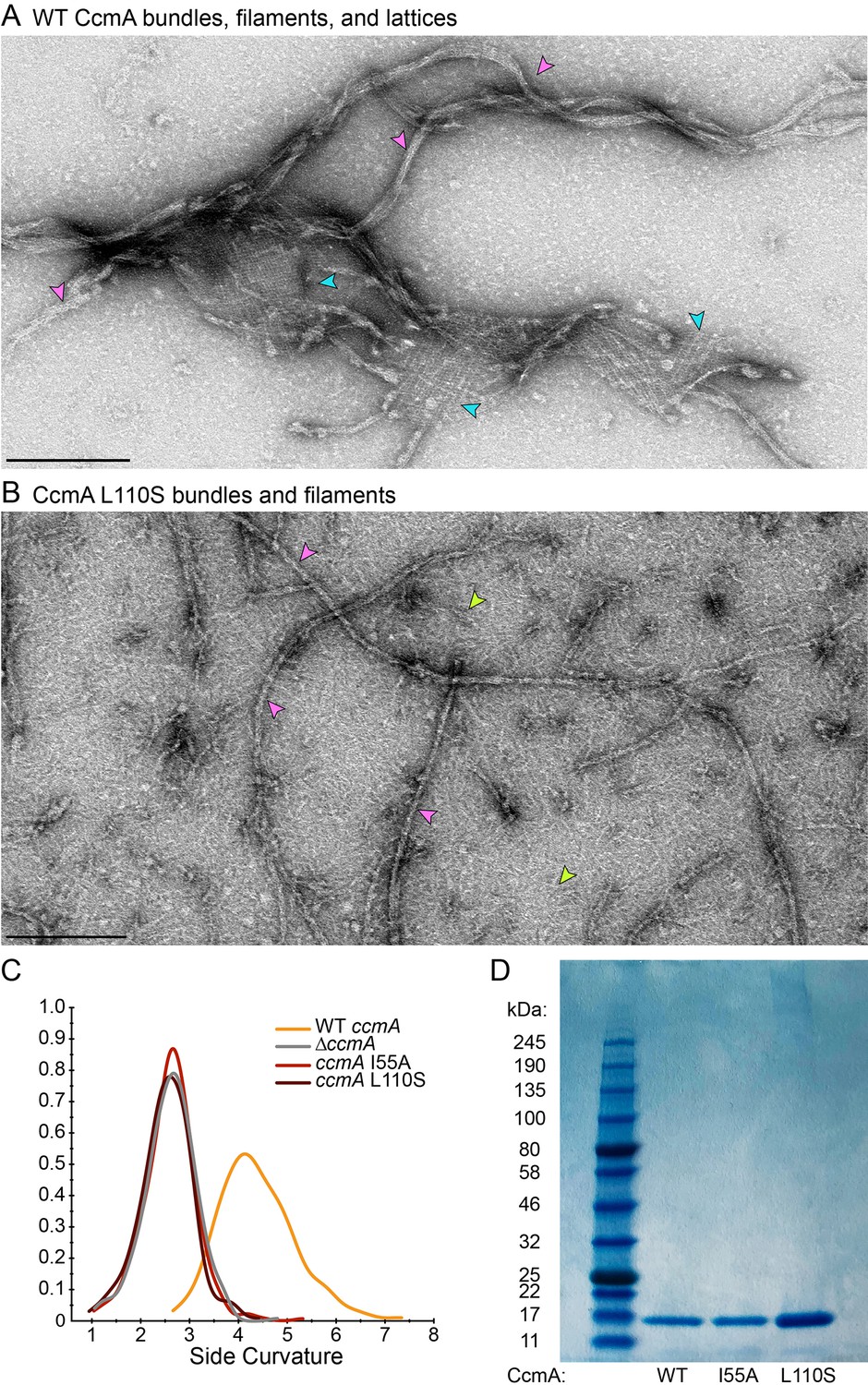
CcmA lattices and bundles.
Negatively stained TEM images of purified CcmA. Scale bars = 200 nm. Lower magnification view than in Figure 8 of (A) wild-type CcmA, displaying both lattices (blue arrows) and extended helical bundles (pink arrows) and (B) CcmAL110S, displaying both individual filaments (lime green arrows) and bundles (pink arrows). (C) Smooth histogram of population side curvature (x-axis) of the cells in Figure 8F (one representative of two biological replicates). (D) Coomassie stained SDS-PAGE gel showing purified wild-type CcmA, CcmAI55A, and CcmAL110S.
Figure 8—figure supplement 2
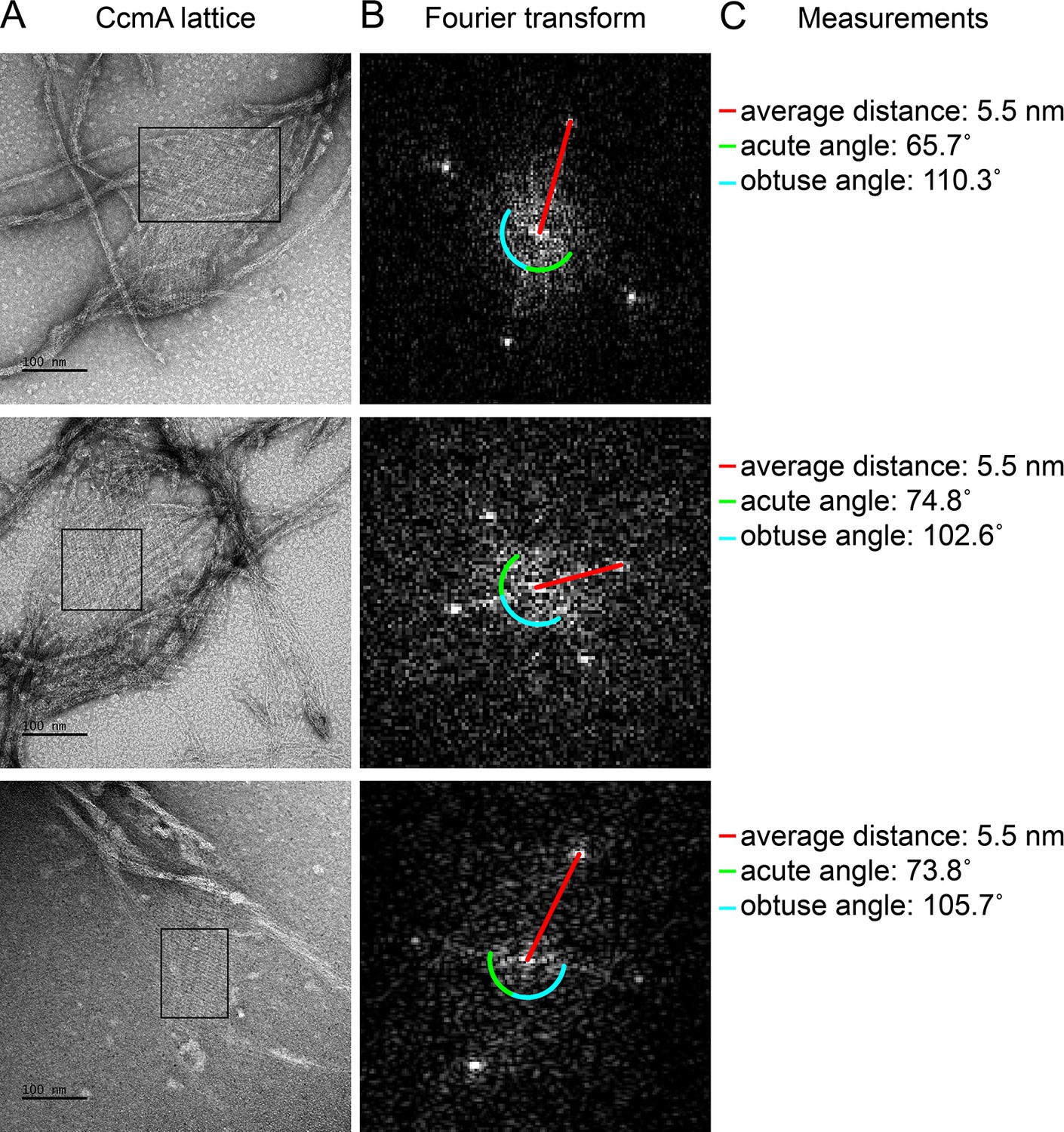
Fourier transform of CcmA lattices shows regular alignment and spacing.
(A) Lattices formed from purified WT CcmA in 25 mM Tris pH 8. Scale bars = 100 nm. (B) Fourier transform of the region inside each corresponding box in (A) performed using Fiji (Schindelin et al., 2012). After transformation, images were adjusted to enhance visualization (min: 134, gamma: 0.53, max: 172). (C) Average distance of bright spots from the center represents the distance between individual filaments in each lattice. Angle measurements between spots indicate the relative orientation of filaments within lattices. Average of the measurements from the three lattices: distance = 5.5 nm; acute angle = 71.5°; obtuse angle = 106.2°. Images shown are from one representative of three biological replicates.
Figure 9 with 2 supplements
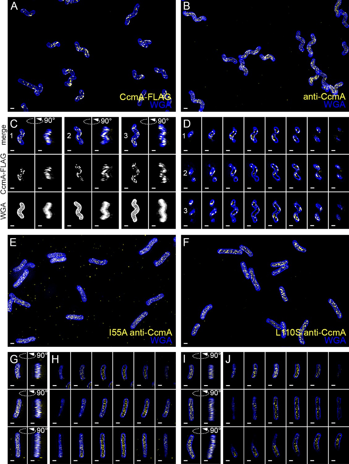
Wild-type CcmA appears as short foci on the side of the cell, but CcmA mutants I55A and L110S appear as foci in the interior of the cell.
3D SIM imaging of CcmA-FLAG cells immunostained with M2 anti-FLAG (A, C, D, yellow) or wild-type or CcmA amino acid substitution mutant cells immunostained with anti-CcmA (B, E–J, yellow); cells counterstained with fluorescent WGA (blue). (A) Color merged maximum projection of CcmA-FLAG immunostained with anti-FLAG and counterstained with fluorescent WGA. (B) Color merged field of view of wild-type cells immunostained with anti-CcmA and counterstained with fluorescent WGA. (C) Top-down (left) and 90-degree rotation (right) 3D views of three individual CcmA-FLAG cells. Top: color merge; middle: anti-FLAG; bottom: fluorescent WGA. (D) Color merged z-stack views of the three CcmA-FLAG cells in (C). (left to right = top to bottom of the cell). Numbering indicates matching cells. (E, F) Color merged field of view of I55A or L110S CcmA, respectively, immunostained with anti-CcmA and counterstained with fluorescent WGA. Top-down (left) and 90-degree rotation (right) 3D views of three individual I55A (G) or L110S (I) cells. (H, J) Color merged z-stack views of the three I55A cells in (G) or L110S cells in (I), respectively (Left to right = top to bottom of the cell). Scale bar = 0.5 µm. The representative images are selected from one of three biological replicates.
Figure 9—figure supplement 1
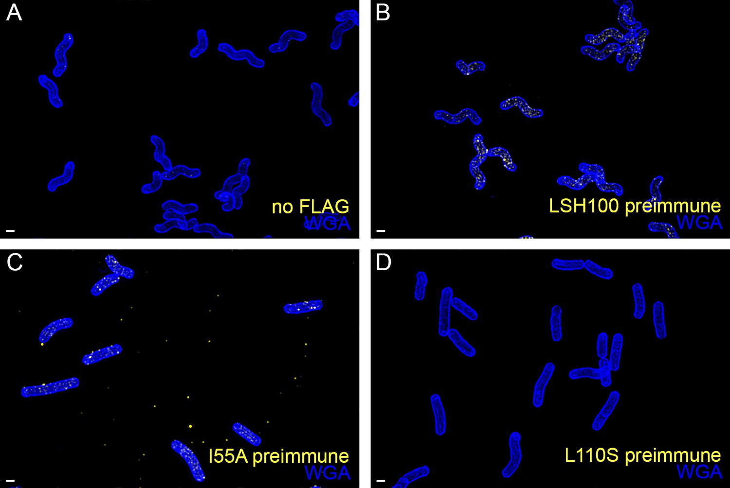
There is low signal in the no-FLAG and preimmune serum controls.
(A) Wild-type (no-FLAG) cells immunostained with M2 anti-FLAG (yellow) and counterstained with fluorescent WGA (blue). (B) Wild-type, (C) I55A, or (D) L110S CcmA cells immunostained with CcmA preimmune serum (yellow) and counterstained with fluorescent WGA (blue). Scale bar = 0.5 µm. The representative images are selected from one of three biological replicates.
Figure 9—video 1
Volumetric rendering and z-slices of the example cells in Figure 9 and three example WT cells immunostained with anti-CcmA and counterstained with fluorescent WGA.
Figure 10 with 3 supplements

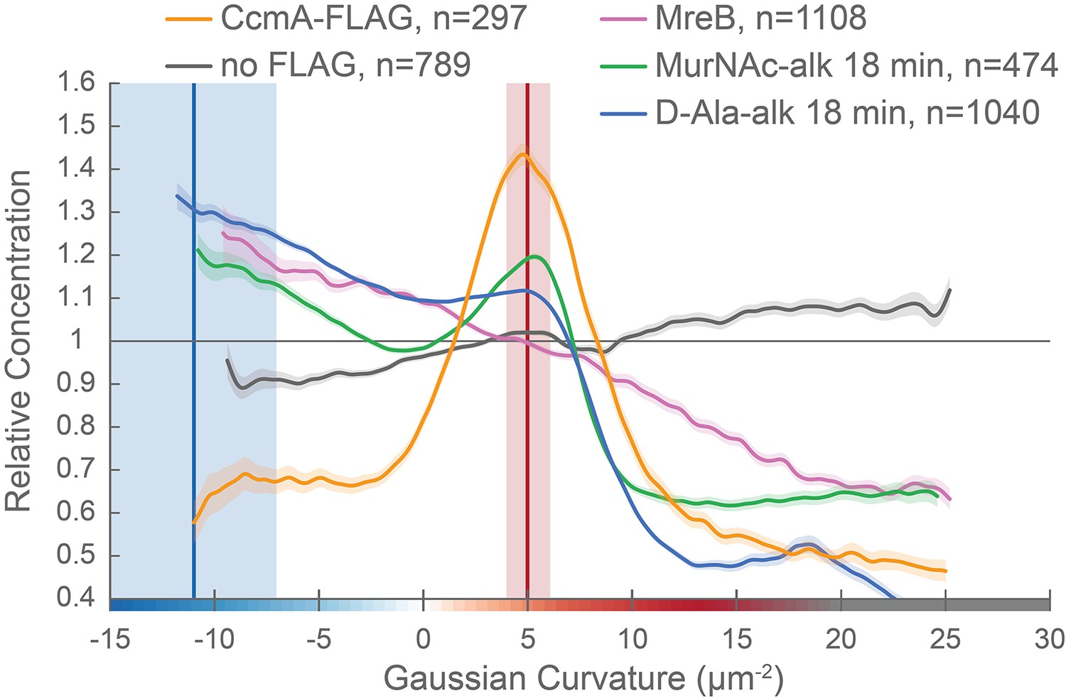
CcmA curvature preference correlates with the peak of new PG incorporation at the major axis area and MreB curvature preference correlates with new PG enrichment at negative Gaussian curvature.
Overlay of sidewall only surface Gaussian curvature enrichment of relative concentration (y-axis) vs. Gaussian curvature (x-axis) from a population of computational cell surface reconstructions with poles excluded of CcmA-FLAG (gold), no-FLAG control (gray), MreB (pink, from Figure 7F), MurNAc-alk (green, from Figure 6C), and D-Ala-alk (blue, from Figure 6C). The represented data are pooled from three biological replicates. Blue and red vertical lines and shaded regions indicate the average ±1 standard deviation Gaussian curvature at the minor and major helical axis, respectively.
Figure 10—figure supplement 1
CcmA is excluded from the poles.
Whole surface (sidewall and poles) Gaussian curvature enrichment of relative signal abundance (y-axis) vs. Gaussian curvature (x-axis) derived from a population of computational cell surface reconstructions of CcmA-FLAG (gold), no-FLAG (gray), MreB (pink, from Figure 7—figure supplement 2), MurNAc-alk (green, from Figure 6B), and D-Ala-alk (blue, from Figure 6B). 90% bootstrap confidence intervals are displayed as a shaded region about each line. The represented data are pooled from three biological replicates. Blue and red vertical lines and shaded regions indicate the average ±1 standard deviation Gaussian curvature at the minor and major helical axis, respectively.
Figure 10—figure supplement 2
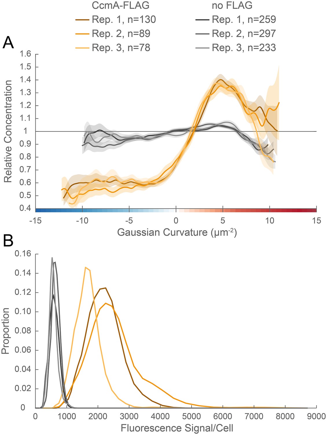
Curvature enrichment analysis of biological replicates of CcmA-FLAG.
(A) Sidewall only surface Gaussian curvature enrichment of relative signal abundance (y-axis) vs. Gaussian curvature (x-axis) of the three biological replicates pooled in Figure 10: CcmA-FLAG (golds) and no-FLAG (grays) cells. 90% bootstrap confidence intervals are displayed as a shaded region about each line. (B) Histogram of fluorescence signal per cell divided by the number of pixels in the projected cell area for the populations in (A).
Figure 10—figure supplement 3
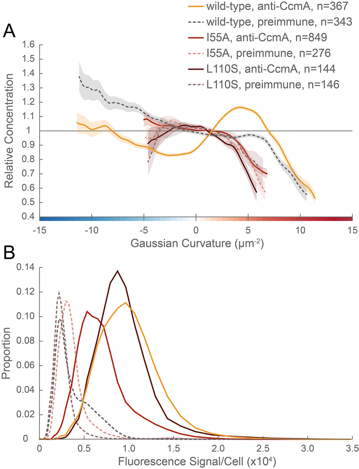
CcmA mutants are not enriched at positive Gaussian curvature.
(A) Sidewall Gaussian curvature enrichment of relative signal abundance (y-axis) vs. Gaussian curvature (x-axis) for a population of computational cell surface reconstructions with poles excluded of wild-type LSH100 cells immunostained with anti-CcmA (gold) or preimmune serum (dotted gray); CcmA I55A cells immunostained with anti-CcmA (red) or preimmune serum (dotted light pink); or CcmA L110S cells immunostained with anti-CcmA (dark red) or preimmune serum (dotted mauve). 90% bootstrap confidence intervals are displayed as a shaded region about each line. (B) Histogram of fluorescence signal per cell divided by the number of pixels in the projected cell area for the populations in (A). The represented data are pooled from three biological replicates.
Figure 11 with 4 supplements
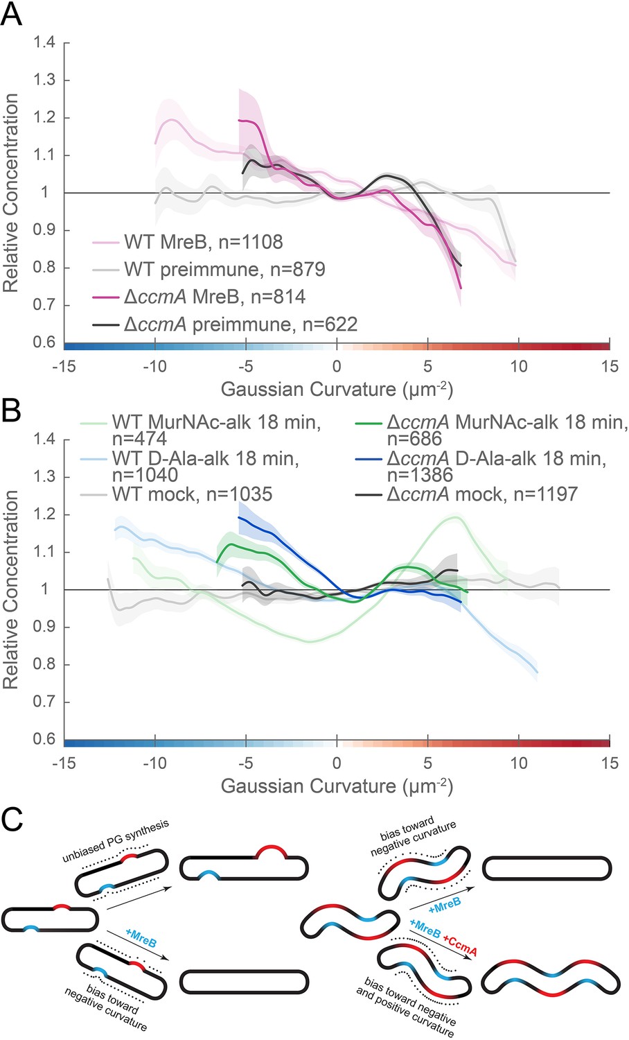
MreB and CcmA contribute to cell wall synthesis patterning.
(A, B) Sidewall only Gaussian curvature enrichment of relative concentration (y-axis) vs. Gaussian curvature (x-axis) from a population of computational cell surface reconstructions of HJH1 (amgK murU) and JTH6 (amgK murU ΔccmA) cells immunostained with (A) anti-MreB (HJH1, light pink; JTH6, dark pink) or preimmune serum (HJH1, light gray; JTH6, dark gray) or (B) 18 min MurNAc-alk (HJH1, light green; JTH6, dark green) or D-Ala-alk (HJH1, light blue; JTH6, dark blue) pulse-labeled or mock-labeled (HJH1, light gray; JTH6, dark gray) cells. 90% bootstrap confidence intervals are displayed as a shaded region about each line. The represented data are pooled from three biological replicates. (C) Model of the contribution of synthesis patterning to rod and helical shape maintenance. Dots indicate different densities of cell wall synthesis that can decrease or propagate non-zero Gaussian curvature. Colored shading indicates local regions of positive (red) and negative (blue) Gaussian curvature.
Figure 11—figure supplement 1
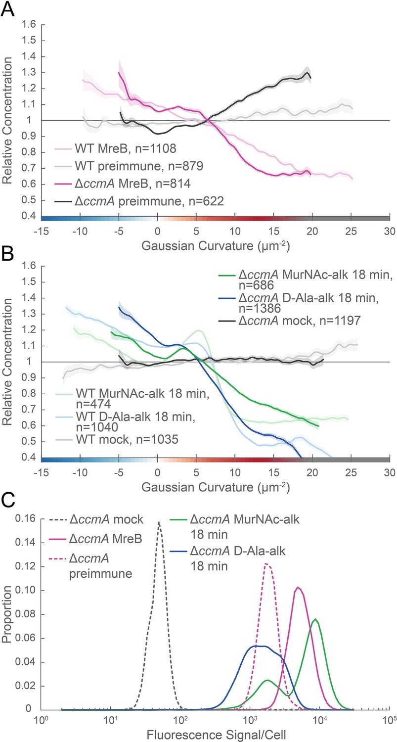
Cell wall synthesis patterning but not MreB curvature preference is altered by loss of CcmA.
(A, B) Whole surface (sidewall and poles) Gaussian curvature enrichment of relative concentration (y-axis) vs. Gaussian curvature (x-axis) from a population of computational cell surface reconstructions of wild-type (WT, HJH1, amgKmurU) and ΔccmA (ΔccmA, JTH6, ΔccmA amgKmurU) of cells immunostained with (A) anti-MreB (wild-type, light pink; ΔccmA, dark pink) or preimmune serum (WT, light gray; ΔccmA, dark gray) or (B) 18 min MurNAc-alk (HJH1, light green; JTH6, dark green) or D-Ala-alk (HJH1, light blue; JTH6, dark blue) pulse-labeled or mock-labeled (HJH1, light gray; JTH6, dark gray) cells. 90% bootstrap confidence intervals are displayed as a shaded region about each line. (C) Histogram of fluorescence signal per cell divided by the number of pixels in the projected cell area for the JTH6 populations in (A) (18 min D-Ala-alk and mock labeling, solid and dotted dark blue, respectively) and (B) (anti-MreB and preimmune immunostaining, solid and dotted dark pink, respectively). The represented data are pooled from three biological replicates.
Figure 11—figure supplement 2
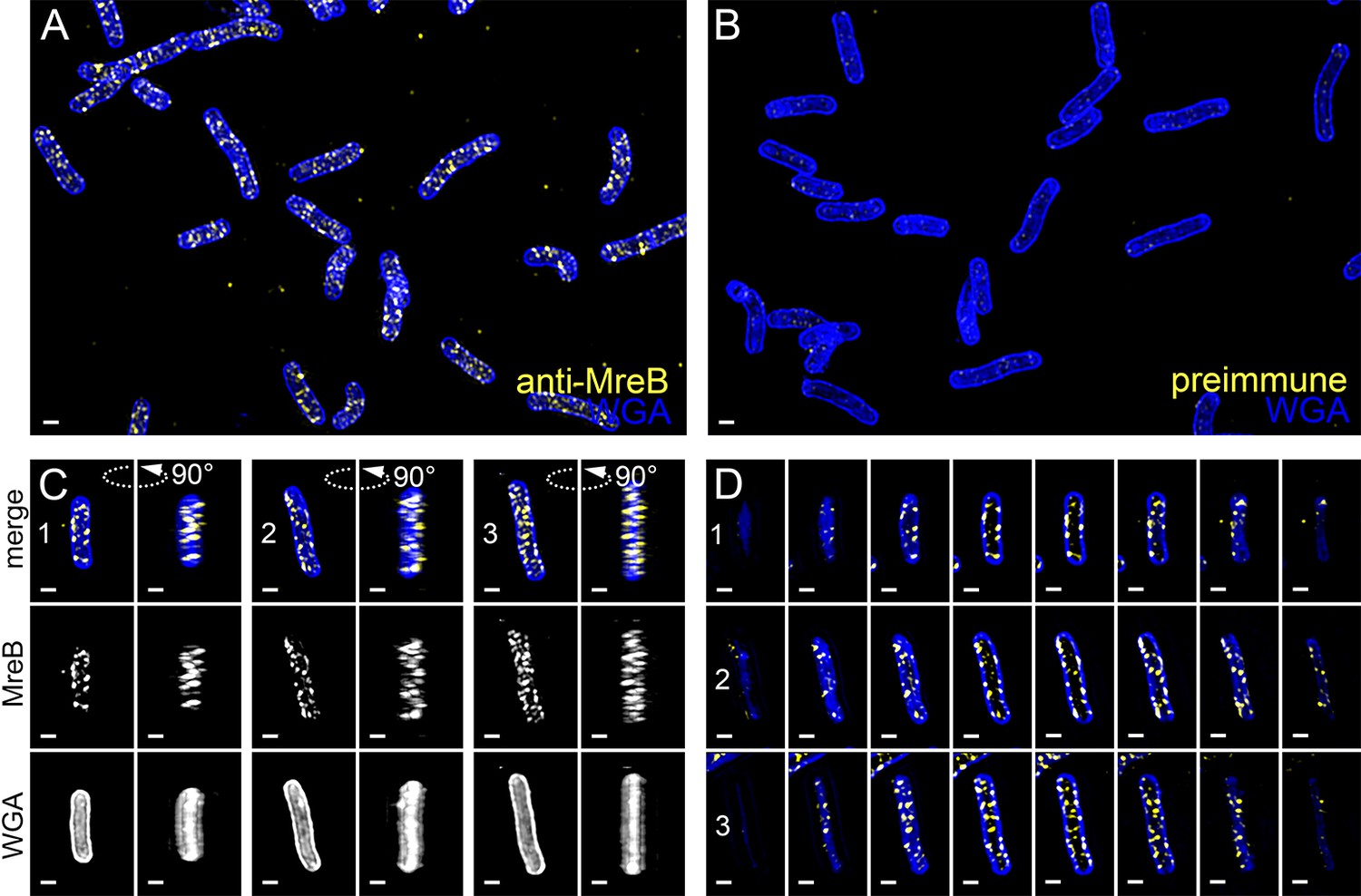
MreB is present as small foci along the sidewall in ΔccmA.
3D SIM imaging of ΔccmA cells immunostained with anti-MreB (A, C, D, yellow) or preimmune serum (B) and counterstained with fluorescent WGA (blue). Color merged maximum projection of anti-MreB (A) or preimmune (B). (C) Top-down (left) and 90-degree rotation (right) 3D views of three individual cells. Top: color merge; middle: anti-MreB; bottom: fluorescent WGA. (D) Color merged z-stack views of the three cells in (C), (left to right = top to bottom of the cell). Numbering indicates matching cells. Scale bar = 0.5 µm. The representative images are selected from one of three biological replicates.
Figure 11—figure supplement 3
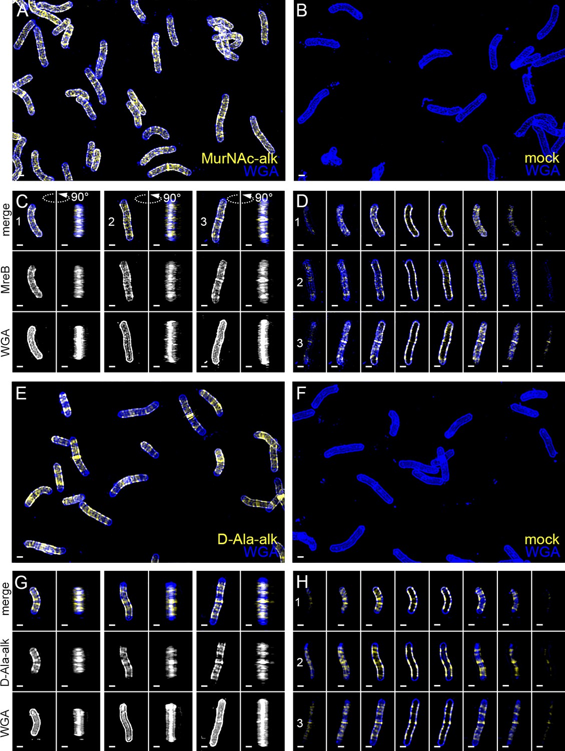
New cell wall growth appears as diffuse labeling and circumferential bands dispersed along the sidewall, excluded from poles, and present at septa in ΔccmA.
3D SIM imaging of ΔccmA cells labeled with an 18 min pulse of MurNAC-alk (A, C, D, yellow) or D-Ala-alk (E, G, H, yellow) or mock labeled (B, F) and counterstained with fluorescent WGA (blue). Color merged maximum projection of MurNAc-alk (A), D-Ala-alk (E), or mock (B, F) labeling with fluorescent WGA counterstain. (C, G) Top-down (left) and 90-degree rotation (right) 3D views of three individual cells, including a dividing cell (C, G), right). Top: color merge; middle: 18 min MurNAc-alk (C) or 18 min D-Ala-alk (G); bottom: fluorescent WGA. (D, H) Color merged z-stack views of the three cells in (C, G), respectively (left to right = top to bottom of the cell). Numbering indicates matching cells. Scale bar = 0.5 µm. The representative images are selected from one of three biological replicates.
Figure 11—video 1
Volumetric rendering and z-slices of the example cells in Figure 11—figure supplements 2 and 3.
Author response image 1
Tables
Table 1
MurNAc-alk incorporation into PG
| Muropeptide (non-reduced) | Theoretical neutral mass | MurNAc-alk labeled H. pylori | Control H. pylori | ||||
|---|---|---|---|---|---|---|---|
| Observed ion (charge) | Rt* (min) | Calculated neutral mass | Observed ion (charge) | Rt* (min) | Calculated neutral mass | ||
| Di | 696.270 | 697.289 (1+) | 20.3 | 696.282 | 697.290 (1+) | 20.4 | 696.283 |
| Alk-Di | 734.286 | 735.307 (1+) | 30.5 | 734.300 | -† | - | - |
| Tri | 868.355 | 869.375 (1+) | 15.8 | 868.368 | 869.374 (1+) | 15.8 | 868.367 |
| Alk-Tri | 906.371 | 907.392 (1+) | 25.8 | 906.385 | - | - | - |
| Tetra | 939.392 | 940.411 (1+) | 20.4 | 939.404 | 940.412 (1+) | 20.4 | 939.405 |
| Alk-Tetra | 977.408 | 978.428 (1+) | 30.4 | 977.421 | - | - | - |
| Penta | 1010.429 | 1011.449 (1+) | 22.9 | 1010.442 | 1011.449 (1+) | 22.8 | 1010.442 |
| Alk-Penta | 1048.445 | 1049.464 (1+) | 32.9 | 1048.457 | - | - | - |
| TetraTri | 1789.736 | 895.889 (2+) | 33.4 | 1789.762 | 895.888 (2+) | 33.3 | 1789.761 |
| Alk-TetraTri | 1827.752 | 914.898 (2+) | 39.2 | 1827.781 | - | - | - |
| TetraTetra | 1860.774 | 931.407 (2+) | 35.0 | 1860.799 | 931.407 (2+) | 34.9 | 1860.799 |
| Alk-TetraTetra | 1898.789 | 950.416 (2+) | 39.7 | 1898.817 | - | - | - |
| TetraPenta | 1931.811 | 966.926 (2+) | 35.8 | 1931.837 | 966.925 (2+) | 35.7 | 1931.835 |
| Alk-TetraPenta | 1969.826 | 985.934 (2+) | 39.9 | 1969.853 | - | - | - |
-
* Rt, retention time.
†-, not detected. Muropeptides detected (confirming incorporation) via LC-MS analysis of MurNAc-alk labeled versus control PG digests. The control cells displayed no evidence of any MurNAc-alk incorporation.
Key resources table
| Reagent type (species) or resource | Designation | Source or reference | Identifiers | Additional information |
|---|---|---|---|---|
| Antibody | Monoclonal ANTI-FLAG M2 antibody produced in mouse | Sigma | Cat# F1804, RRID:AB_262044 | IF(1:200) |
| Antibody | Goat anti-Mouse IgG (H+L) Highly Cross-Adsorbed Secondary Antibody, Alexa Fluor 488 | Invitrogen | Cat# A-11029, RRID:AB_2534088 | IF(1:200) |
| Antibody | Goat anti-Rabbit IgG (H+L) Cross-Adsorbed Secondary Antibody, Alexa Fluor 488 | Invitrogen | Cat#: A-11008; RRID: AB_143165 | IF(1:200) |
| Antibody | Polyclonal rabbit αCcmA | (Blair et al., 2018) | IF (1:200); WB (1:10,000) | |
| Antibody | Polyclonal rabbit αMreB (H. pylori) | (Nakano et al., 2012) | IF (1:500); WB (1:25,000) | |
| Commercial assay, kit | Click-iT Cell Reaction Buffer Kit | Invitrogen | Cat# C10269 | |
| Chemical compound, drug | Alexa Fluor 555 Azide, Triethylammonium Salt | Invitrogen | Cat# A20012 | |
| Chemical compound, drug | D-Ala-alk ((R)−2-Amino-4-pentynoic acid) | Boaopharma | Cat# B60090 | |
| Chemical compound, drug | MurNAc-alk | (Liang et al., 2017) | ||
| Chemical compound, drug | MurNAc | Sigma | Cat# A3007 | |
| Chemical compound, drug | Wheat Germ Agglutinin, Alexa Fluor 488 Conjugate | Invitrogen | Cat# W11261 | |
| Chemical compound, drug | Wheat Germ Agglutinin, Alexa Fluor 555 Conjugate | Invitrogen | Cat# W32464 | |
| Other | ProLong Diamond Antifade Mountant | Invitrogen | P36961 |
Table 2
Strains used in this study.
| Strain | Genotype/description | Construction | Reference |
|---|---|---|---|
| LSH100 | Wild-type: mouse-adapted G27 derivative | - | Lowenthal et al., 2009 |
| LSH141 (Δcsd2) | LSH100 csd2::cat | - | Sycuro et al., 2010 |
| TSH17 (Δcsd6) | LSH100 csd6::cat | - | Sycuro et al., 2013 |
| LSH108 | LSH100 rdxA::aphA3sacB | - | Sycuro et al., 2010 |
| HMJ_Ec_pLC292-KU | E. coli TOP10 pLC292-KU | Transformation of TOP10 with pLC292-KU | This study |
| HJH1 | LSH100 rdxA::amgKmurU | Integration of pLC292-KU into LSH108 | This study |
| IM4 | LSH100 mcGee:mreB | Integration of pIM04into LSH100 | This study |
| JTH3 | LSH100 ccmA:2X-FLAG:aphA3 | - | Blair et al., 2018 |
| JTH5 | LSH100 ccmA:2X-FLAG:aphA3 rdxA::amgKmurU | Natural transformation of HJH1 with JTH3 genomic DNA | This study |
| KGH10 | NSH57 ccmA::catsacB | - | Sycuro et al., 2010 |
| LSH117 | LSH100 ccmA::catsacB | Natural transformation of LSH100 with KGH10 genomic DNA | This study |
| SSH1 | LSH100 ccmAI55A | Natural transformation with ccmA I55A PCR product | This study |
| SSH2 | LSH100 ccmAL110S | Natural transformation with ccmA L110S PCR product | This study |
| LSH142 (ΔccmA) | LSH100 ccmA::cat | - | Sycuro et al., 2010 |
| JTH6 | LSH100 rdxA::amgKmurU ccmA::cat | Natural transformation of HJH1 with LSH142 genomic DNA | This study |
Table 3
Primers used in this study.
| Primer name | Sequence (5’ to 3’) |
|---|---|
| AmgK_BamHI_F | GATAGGATCCTGACCCGCTTGACGGCTA |
| MurU_HindIII_R | GTATAAGCTTTCAGGCGCGCTCGC |
| RdxA_F1P1 | CAATTGCGTTATCCCAGC |
| RdxA_dnstm_RP2 | AAGGTCGCTTGCTCAATC |
| O#9 ProMreB (KpnI_5’) | TATTGGTACCCGCTTGATGTATTCATCAAAG |
| O#10 ProMreB_R | GATTAATTTGCTAAAAATCATAAAATAAACTCCTTGTTTTG |
| O#11 ProMreB_F | CAAAACAAGGAGTTTATTTTATGATTTTTAGCAAATTAATC |
| O#12 ProMreB (XhoI_3’) | TATTCTCGAGTTATTCACTAAAACCCACAC |
| O#36 pMcGee-Insert-F | CTGCCTCCTCATCCTCTTCATCCTC |
| O#45 MreBC-seq-F2 | GCACCTATTTTGGGGTTTGAAACC |
| O#47 MreB-seq-F2 | CATTGAGCGCTGGTTTTAAGGCGGTC |
| O#28 MreBseq-F3 | CGATCGTGTTAGTCAAAGGGCAGGGC |
| O#37 pMcGee-Insert-R | GGTGTACAAACATTTAAAGGTAGAG |
| O#68 McGee-1F | CATTTCCCCGAAAAGTGCCACGAGCTCGAAGGAGTATTGATGAAAAAGG |
| O#69 McGee-1R | CTAGAGCGGCCCCACCGCGGCCATCATTAACATCATTATCG |
| O#70 MCS-kan-F | CTCGAGGGGGGGCCCGGTACCCACAGAATTACTCTATGAAGC |
| O#71 MCS-kan-R | CCATTCTAGGCACTTATCCCCTAAAACAATTCATCCAGTAA |
| O#72 McGee-2F | TTACTGGATGAATTGTTTTAGGGGATAAGTGCCTAGAATGG |
| O#73 McGee-2R | CGGATATTATCGTGAGATCGCTGCAGACTGGGGGGAAACTCATGGG |
| O#74 McGee-R6K-F | CCCATGAGTTTCCCCCCAGTCTGCAGCGATCTCACGATAATATCCG |
| O#75 McGee-R6K-R | GTAACTGTCAGACCAAGTTTACTGCGGCCGCGCAAGATCCGGCCACGATGCG |
| O#76 R6K-amp-F | CGCATCGTGGCCGGATCTTGCGCGGCCGCAGTAAACTTGGTCTGACAGTTAC |
| O#77 R6K-amp-R | CCTTTTTCATCAATACTCCTTCGAGCTCGTGGCACTTTTCGGGGAAATG |
| O#78 MCS fragment | CCGCGGTGGGGCCGCTCTAGAACTAGTGGATCCCCCGGGCTGCGGAATTCGCTTATCG |
| O#79 McGee-MCS-F | CGATAATGATGTTAATGATGGCCGCGGTGGGGCCGCTCTAG |
| O#80 McGee-MCS-R | GCTTCATAGAGTAATTCTGTGGGTACCGGGCCCCCCCTCGAG |
| Csd1F | GAGTCGTTACATTAATGTGCATATCT |
| G1480_DnStrmP2 | AAGGGTGCAATAACGCGCTAA |
| MreB_start_F | ATGATTTTTAGCAAATTAATCGG |
| MreB_cat_up_R | CACTTTTCAATCTATATCCGTGCCTCCGCCAATATC |
| C1 | GATATAGATTGAAAAGTGGAT |
| C2 | TTATCAGTGCGACAAACTGGG |
| Cat_mreB_dn_F | AGTTTGTCGCACTGATAAACTGAAATTGGCG |
| MreB_end_R | TTATTCACTAAAACCCACACGGCTGA |
| FabZ_up_F | GCTATCCCATGCTATTGATAGAC |
| Cat_mid_R | GTCGATTGATGATCGTTGTAACTCC |
| MreB_mid_dn_F | GATCAAAGCATCGTGGAATACATCC |
| Supp2_junc1_R_mid | AATTTGCTAAAAATCACTAA |
| MreB_up | AATACCAGCAACTTTTCAAAA |
| Supp1_Junction1_R | ATTTGCTAAAAACACACGGC |
| Catout | CCTCCGTAAATTCCGATTTGT |
| McGee_187 | GCGAGTATTACCACAAGTTTTC |
| CcmA SDM mi R | AGACTAGATTGGATCATTCCCTATTTATTTTCAATTTTCT |
| CcmA SDM mi F | ATAAAGAAAGGAGCATCAGATGGCAATCTTTGATAACAAT |
| CcmA SDM up R | ATTGTTATCAAAGATTGCCATCTGATGCTCCTTTCTTTAT |
| CcmA SDM dn F | AGAAAATTGAAAATAAATAGGGAATGATCCAATCTAGTCT |
| CcmA SDM dn R | GCTCATTTGAGTGGTGGGAT |
| SDM 155A F | ATTCTAAAAGCACGGTGGTGgcCGGACAAACCGGCTCGGTAG |
| SDM 155A R | CTACCGAGCCGGTTTGTCCGgcCACCACCGTGCTTTTAGAAT |
| SDM L110S F | TGGTGGAAAGGAAGGGGATTtcGATTGGGGAAACTCGCCCTA |
| SDM L110S R | TAGGGCGAGTTTCCCCAATCgaAATCCCCTTCCTTTCCACCA |
Additional files
Download links
A two-part list of links to download the article, or parts of the article, in various formats.
Downloads (link to download the article as PDF)
Open citations (links to open the citations from this article in various online reference manager services)
Cite this article (links to download the citations from this article in formats compatible with various reference manager tools)
Distinct cytoskeletal proteins define zones of enhanced cell wall synthesis in Helicobacter pylori
eLife 9:e52482.
https://doi.org/10.7554/eLife.52482


