Figures and data in Shape selection and mis-assembly in viral capsid formation by elastic frustration

Figures
Tables
Additional files

7 figures, 1 table and 1 additional file

Figures

Figure 1

Download asset Open asset

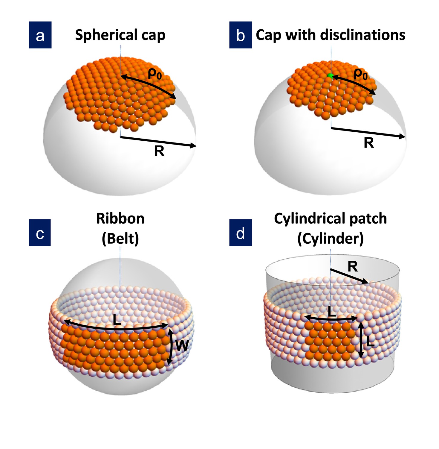
Sketch of the different structures considered in this study.

(a) A hexagonally-ordered spherical cap of radius $R$ and geodesic radius $ρ_{0}$ without defects; (b) a spherical cap with a single disclination at the center (as shown) or multiple disclinations; (c) a rectangular ribbon with length $L$ and width $W$ , that it is called *belt* when the length becomes $L = 2 π R$ ; and (d) a cylindrical patch with size $L$ , that eventually becomes a cylinder of radius $R$ . In the bending-dominated regime, $R = R_{0}$ .

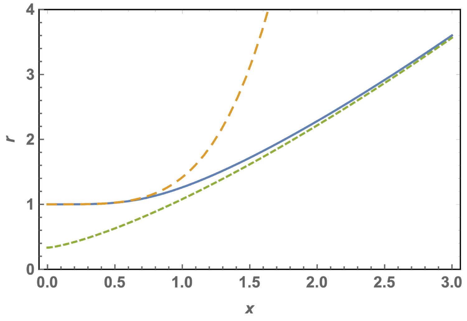
Figure 2

Download asset Open asset

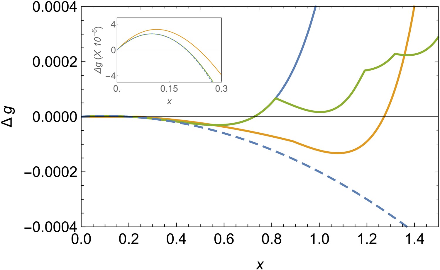
Comparison of free energy landscapes for different structures.

Free energy of formation $Δ g$ versus the radius of the patch x in the bending-dominated regime for a defectless spherical shell (blue line), a spherical shell with defects (green), and a ribbon/belt (orange) for $λ = 0.0001$ and $Δ \tilde{μ} = 0.001$ . The optimal structure is the one with the minimum energy, which is the belt in this case. The dashed line represents the unfrustrated decrease of energy expected by the classical nucleation picture for the defectless spherical cap in the absence of elastic stresses. The inset zooms the nucleation barrier located at small patch sizes.

Figure 3

Download asset Open asset

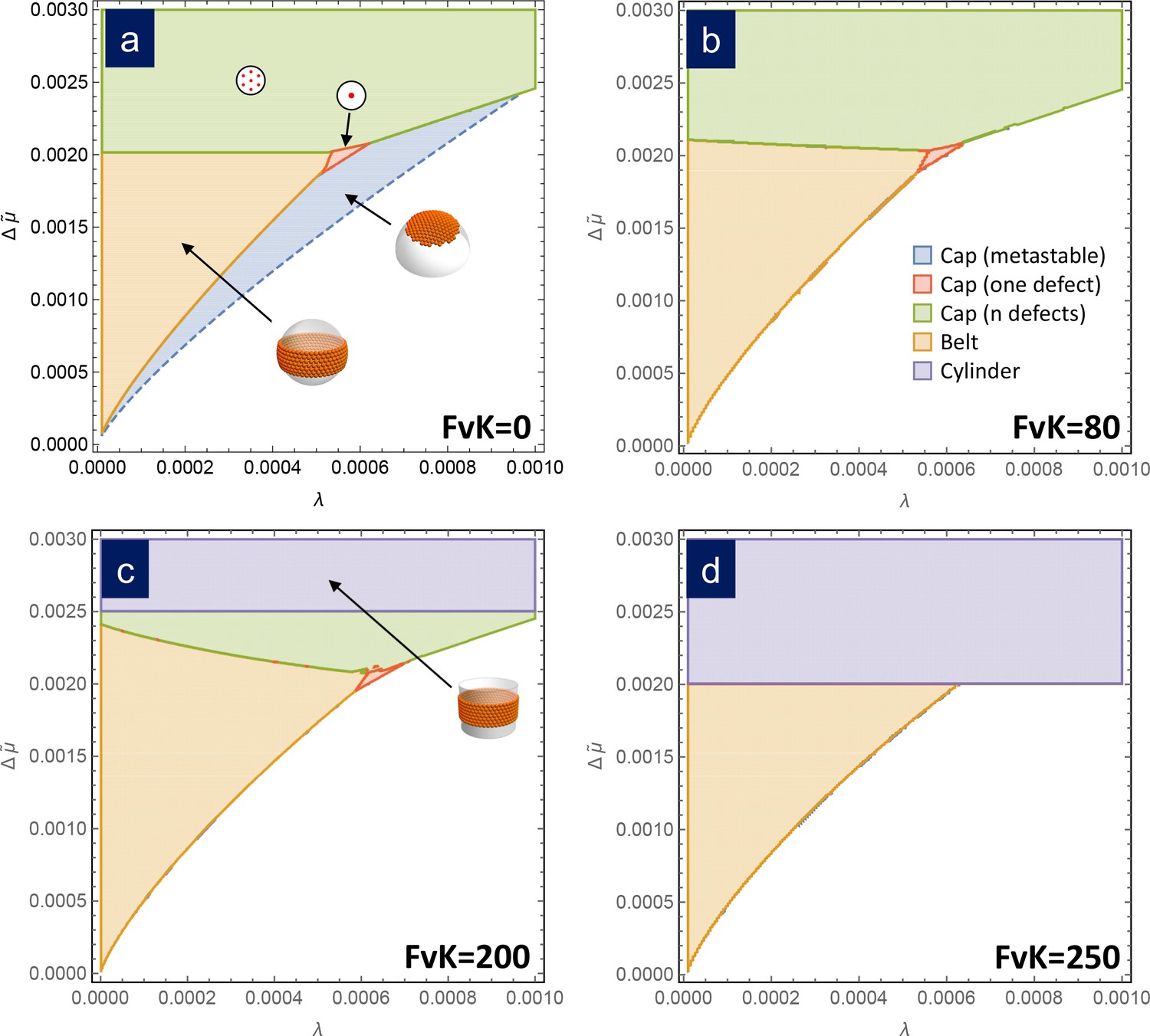
Assembly phase diagrams.

Phase diagrams of the most stable structures in terms of the scaled chemical potential $Δ \tilde{μ}$ and the scaled line tension $λ$ for different values of the FvK number: a) $γ = 0$ , corresponding to the bending-dominated regime, (b) $γ = 80$ , (c) $γ = 200$ , and d) $γ = 250$ . Three possible equilibrium regions are present: belts (i.e. closed ribbons, in orange), frustrated capsids with one defect (red), closed shells with defects (green), and cylinders (purple). Additionally, a region corresponding to a metastable spherical cap without defects (blue) is shown only in (a). In the white region, the equilibrium state corresponds to disaggregated individual capsomers.

Figure 4

Download asset Open asset

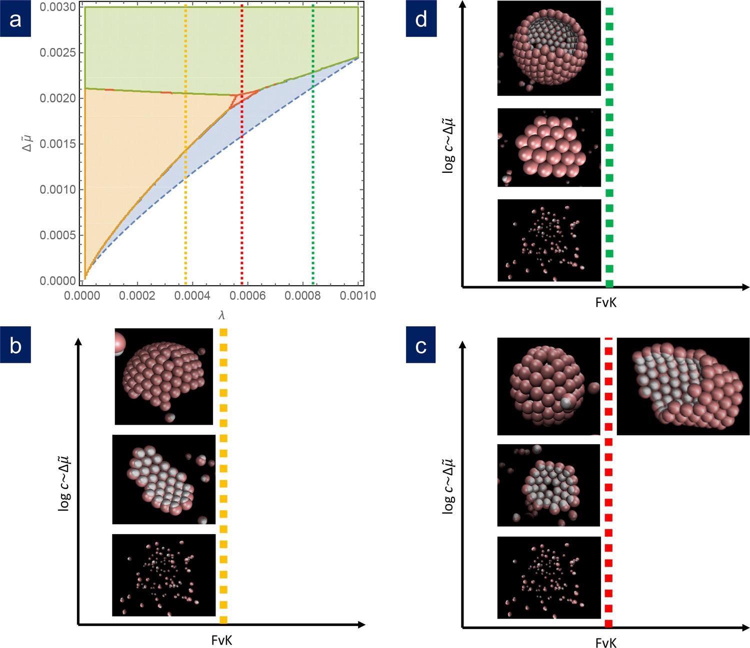
Comparison of simulation results with the theoretical phase diagram.

(a) Phase diagram of the most stable structure in terms of the scaled chemical potential $Δ \tilde{μ}$ and the scaled line tension $λ$ for $γ = 80$ . Snapshots of the final outcome of the simulation for different initial capsomer concentrations for: b) $λ = 0.00037$ , obtained with $ν = 1.45$ and a $m = 36$ , $n = 18$ potential. By increasing the concentration of capsomers one goes from a dissassembled state to the formation of a ribbon to a spherical shell with defects. (The ribbon and spherical shell are not closed in the snapshots due to the limited number of capsomers and finite simulation time). (c) $λ = 0.000525$ , obtained with $ν = 1.38$ and a $m = 36$ , $n = 18$ potential. As concentration increases, one goes from a shell with one defect to a complete shell with many defects. By increasing the FvK number to $γ = 1280$ (by setting $α = 0.4$ ), the simulations clearly forms cylindrical tubes. (d) $λ = 0.00084$ , obtained with $ν = 1.45$ and a $m = 24$ , $n = 12$ potential. In this case, the sequence is: disagreggated, metastable defectless shell, and closed spherical shell with many defects (a partial shell is shown). The simulation results agree qualitatively with the predictions from the theoretical phase diagram.

Appendix 1—figure 1

Download asset Open asset

Free energy of formation $Δ g_{c a p}$ of a spherical cap without defects, Equation A4, versus the radius of the patch $x$ for $λ = 0.0001$ and different values of the scaled chemical potential $Δ \tilde{μ}$ , illustrating the situations in which no assembly is possible (short dashed line, $Δ \tilde{μ} = 0.0002$ ), a geometrically frustrated metastastable cap (dashed line, $Δ \tilde{μ} = 0.0005$ ) or stable (solid line, $Δ \tilde{μ} = 0.001$ ) finite shell.

Appendix 1—figure 2

Download asset Open asset

Scaled optimal radius $r$ of a spherical cap without defects as a function of the patch size $x$ for a FvK number $γ = 80$ .

The solid line is the exact solution, Equation A29, the short dashed line is the approximation for large shells or FvK, Equation A31, and the dashed line is the approximation for small shells or FvK, Equation A30.

Appendix 1—figure 3

Download asset Open asset

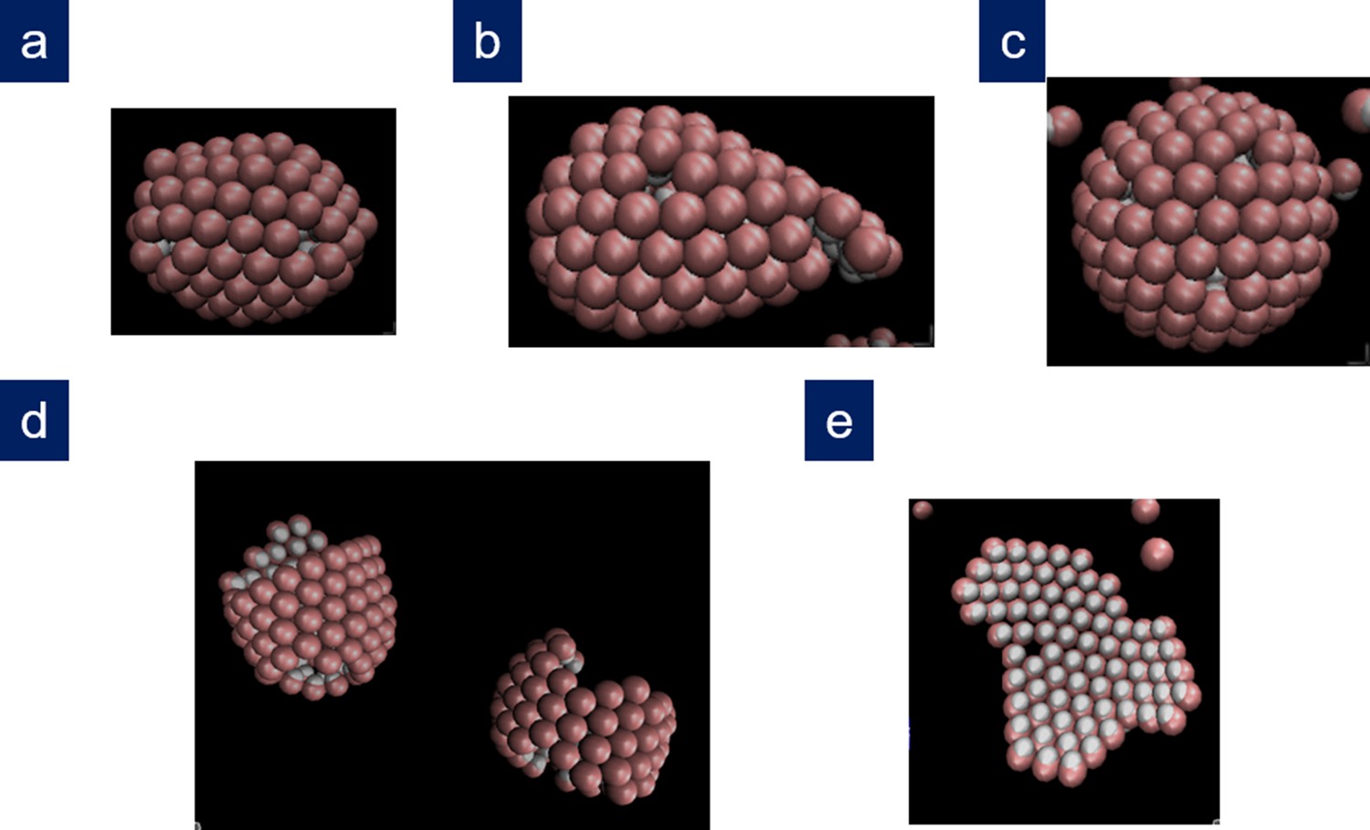
Other structures obtained in the simulations.

(a) Bullet-shaped shell and (b) conical shell obtained in two different repetitions for $γ = 224$ , $λ = 0.00069$ , with $m = 36$ , $n = 18$ , $ν = 1.345$ , $α = 0.4$ and $ρ = 0.02$ ; (c) T = 13 icosahedral shell obtained for $γ = 100$ , $λ = 0.0005246$ , with $m = 36$ , $n = 18$ , $ν = 1.40$ , $α = 0.1$ and $ρ = 0.02$ ; (d) coexistence between a cylinder and a partial spherocylindrical shell obtained for $γ = 900$ , $λ = 0.0005246$ , with $m = 36$ , $n = 18$ , $ν = 1.40$ , $α = 0.3$ and $ρ = 0.02$ ; (e) branched ribbon-like structure (Köhler et al., 2016) obtained at low values of the scaled line tension for $γ = 71$ , $λ = 0.00031$ , with $m = 36$ , $n = 18$ , $ν = 1.47$ , $α = 0.1$ and $ρ = 0.0125$ .

Tables

Table 1

Estimates of the main geometric and elastic properties of different non-enveloped empty viral capsids.

The Young’s modulus $E$ has been evaluated from AFM nanoindentation experiments (Mateu, 2012; Michel et al., 2006; Ivanovska et al., 2007; Sae-Ueng et al., 2014) and, for SV40, from the experimental spring constant (van Rosmalen et al., 2018) using the standard thin shell formula $k = 2.25 E h^{2} / R$ (Ivanovska et al., 2004). The 2D Young’s Modulus was calculated as $Y = E h$ ; the effective diameter of the capsomers as (Santolaria, 2011) $σ = R / \sqrt{\frac{5 \sqrt{3}}{π}} (T + \frac{1}{\sqrt{3}} c o t (\frac{π}{5}) - 1)$ , where $T$ is the triangulation number; the line tension as (Luque et al., 2012) $λ = \frac{2 ϵ_{0}}{\sqrt{3} σ}$ considering a typical binding energy $ϵ_{0} \approx 10 k_{B} T$ ; and the FvK number as $γ = 12 (1 - ν_{p}^{2}) (R / h)^{2}$ , with $ν_{p} = 0.3$ (Buenemann and Lenz, 2008).

Virus	T-number	Diameter (nm)	Thickness h (nm)	E (Gpa)	Y (N/m)	σ (nm)	Scaled line tension λ	Föppl-von Karman γ
CCMV	3	28	3.8	0.14	0.53	5.9	0.00107	148
λ Procapsid	7	50	4.0	0.16	0.64	6.8	0.000436	427
λ Capsid	7	63	1.8	1.0	1.8	8.6	0.0000976	3344
SV40	7	45	6.0	0.033	0.2	6.1	0.00174	152

Additional files

Transparent reporting form: https://cdn.elifesciences.org/articles/52525/elife-52525-transrepform-v2.pdf
Download elife-52525-transrepform-v2.pdf

Download links

A two-part list of links to download the article, or parts of the article, in various formats.

Downloads (link to download the article as PDF)

Article PDF

Open citations (links to open the citations from this article in various online reference manager services)

Mendeley

Cite this article (links to download the citations from this article in formats compatible with various reference manager tools)

Carlos I Mendoza
David Reguera

(2020)

Shape selection and mis-assembly in viral capsid formation by elastic frustration

eLife 9:e52525.

https://doi.org/10.7554/eLife.52525

Share this article

Cite this article

Sketch of the different structures considered in this study.

Comparison of free energy landscapes for different structures.

Assembly phase diagrams.

Comparison of simulation results with the theoretical phase diagram.

Scaled optimal radius r of a spherical cap without defects as a function of the patch size x for a FvK number γ=80.

Other structures obtained in the simulations.

Estimates of the main geometric and elastic properties of different non-enveloped empty viral capsids.

Transparent reporting form

Downloads (link to download the article as PDF)

Open citations (links to open the citations from this article in various online reference manager services)

Cite this article (links to download the citations from this article in formats compatible with various reference manager tools)

Scaled optimal radius $r$ of a spherical cap without defects as a function of the patch size $x$ for a FvK number $γ = 80$ .