Quantitative properties of a feedback circuit predict frequency-dependent pattern separation
- Institute for Experimental Epileptology and Cognition Research, University of Bonn, Germany
- International Max Planck Research School for Brain and Behavior, University of Bonn, Germany
- Deutsches Zentrum für Neurodegenerative Erkrankungen e.V., Germany
Figures
Figure 1 with 1 supplement

Recruitment of feedback inhibition assessed using population Ca2+ imaging.
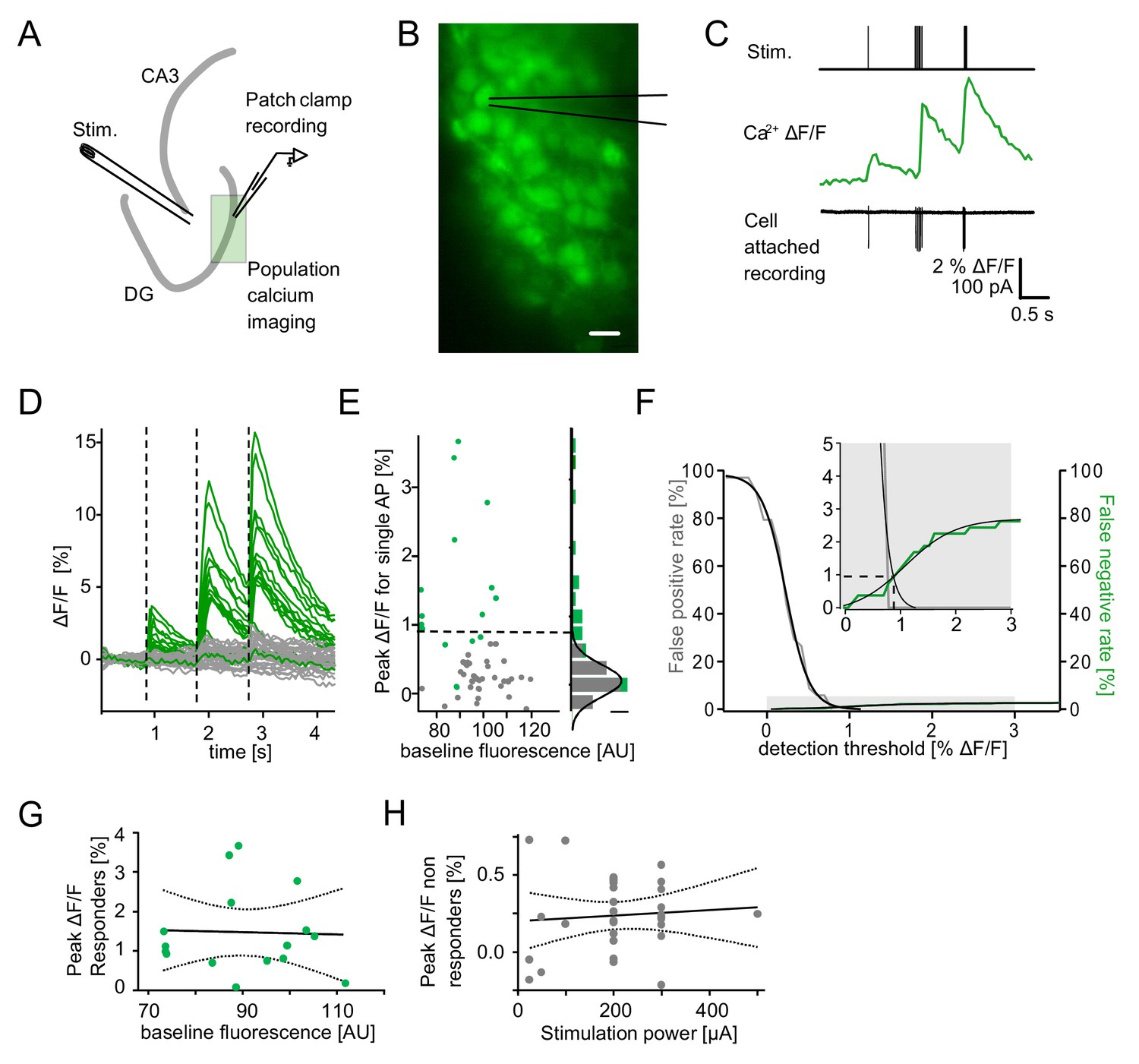
Combined population Ca2+ imaging and IPSC recordings of GCs during antidromic electrical stimulation. (A) Schematic illustration of the experimental setup. Dashed lines represent cuts to sever CA3 backprojections. (B) Top: reconstruction of the dendritic tree of a representative GC. Bottom: Feedback IPSC at increasing stimulation strength during stratum lucidum stimulation. (C) IPSCs were completely blocked by GABAzine and CNQX + D-APV and largely by DCG-IV. (D) Left: overlay of exemplary OGB1-AM-loaded GC population (green) with a ΔF/F map (white). right: traces of ΔF/F over time of a subpopulation of cells depicted on the left. (E) Simultaneous cell attached recording and calcium imaging to measure the action potential induced somatic calcium transient amplitude. (F) Scatterplot and histogram of the calcium fluorescence peaks of cells which either did (green) or did not (grey) fire action potentials, as assessed by cell attached recordings. (G) Illustration of the anatomical localization of maximum connectivity plane slices. Short black dashed lines indicate depth at which the slice plane is aligned to the dorsal brain surface. (H) Antidromic stimulation elicited Ca2+ transients primarily at this depth (black bars). (I) Normalized IPSC amplitude and activated cell fraction both increase with increasing stimulation strength (example from a single slice). (J) Summary of all slices (K) Summary data plotted to show the increase of inhibition as a function of the active GC fraction.
Figure 1—figure supplement 1
Detection of single action potential induced calcium transients.
A section of the dentate gyrus was loaded with OGB1-AM and imaged with multibeam two-photon microscopy while antidromically eliciting action potentials and recording from individual cells in cell-attached mode. (A) A schematic illustration of the experimental setup. (B) Example of OGB1-AM loaded GCs. Scale bar: 10 µm (C) Cells were stimulated with a single pulse (left) or bursts of 5 pulses at 30 Hz (middle) or 100 Hz (right). Cell attached recordings revealed the exact number of induced action potentials (bottom), which could then be correlated with the intracellular calcium signal (middle). (D) Superposition of the calcium fluorescence traces of 49 recorded cells constituted of cells identified as responders (green) or non-responders (grey) by cell attached recordings. (E) Peak ΔF/F for single APs of identified responders and non-responders plotted against their respective baseline fluorescence (left). A histogram of the peak ΔF/F of both groups fitted with a Gaussian distribution of the non-responders (right, scale bar = 5 cells). The dashed line indicates detection threshold at the quadruple standard deviation of this fit (0.94% ΔF/F). (F) False-positive (gray) and false-negative (green) rates were plotted as a function of the detection threshold and fitted with sigmoidal functions. A detection threshold of 0.94% leads to exactly equal numbers of false positives and false negatives if the actually active fraction of GCs is 3% (inset, dashed lines). (G) To test for potential effects of variable dye loading on detection efficacy, we tested for a correlation between peak ΔF/F of responders and baseline fluorescence intensity (p>0.05). (H) To test if increasing numbers of responders at increasing stimulation power led to increases of false positives in the densely packed GC layer, we correlated peak ΔF/F of non-responders with stimulation power (p>0.05). Dashed lines in (G) and (H) represent the 95% confidence intervals of linear regressions.
Figure 2 with 3 supplements
Recruitment of feedback inhibition assessed optogenetically.
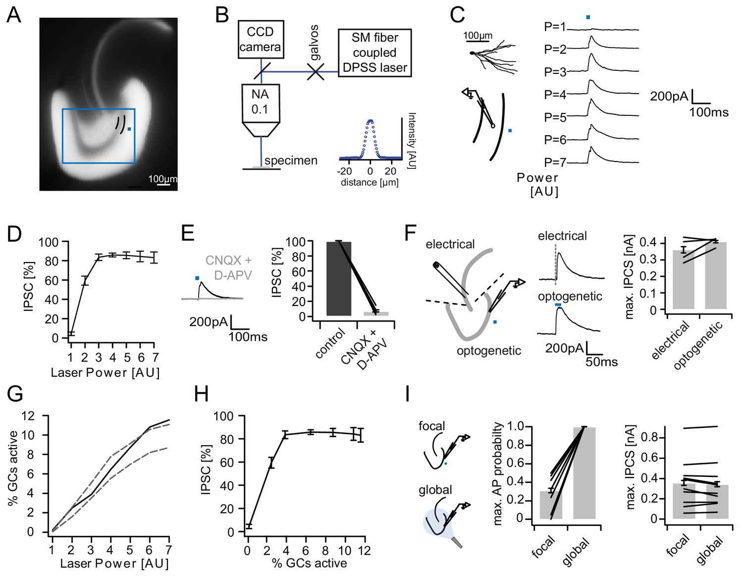
(A) EYFP fluorescence in dentate GCs of Prox1/ChR2(H134R)-EYFP transgenic mice. The field of view for rapid focal optogenetic stimulation is indicated by a blue square. A typical stimulation site approx. 40 µm from the GC layer (two short black lines) is indicated by a blue dot. (B) Schematic of the microscope setup used to achieve spatially controlled illumination. The inset shows the intensity profile of the laser spot. (C) Top left, reconstruction of an Alexa594 filled GC. Left, illustration of optical stimulation. Right, IPSCs following 20 ms light pulses at increasing laser power (p=1 to 7 AU). Each trace represents an average of three trials. (D) Summary of IPSC amplitudes from cells in the superior blade (n = 7 cells). IPSC amplitudes were normalized to the maximum amplitude within each cell. (E) Optogenetically elicited IPSCs are abolished by glutamatergic blockers (40 µM CNQX + 50 µM D-APV, n = 9). (F) Left, Schematic of focal optical and electrical stimulation. Dashed lines indicate cuts to sever CA3 backprojections. Middle, Example traces for IPSCs following electrical or focal optogenetic stimulation. Right, maximal IPSC amplitude for the two stimulation paradigms (361 ± 37 vs. 410 ± 13 pA for electrical and optogenetic stimulation respectively, paired t-test, p=0.28, n = 4) (G) The optogenetically activated GC fraction responsible for recruiting the IPSC at the respective laser powers was estimated from systematic cell attached recordings (see Figure 2—figure supplement 1 for details). The best estimate (black) incorporates measurements of the 3D light intensity profile in the acute slice. Upper and lower bounds were estimated by assuming no firing probability decay with increasing slice depth (upper grey dashed line) or isometric firing probability decay (lower grey dashed line. (H) Data from (D) and (H, best estimate) plotted to show the recruitment of feedback inhibition. (I) Comparison of focal optogenetic stimulation to global (light fiber mediated) optogenetic stimulation. Left, Schematic illustration. Middle, Comparison of the AP probability of individual GCs at maximal stimulation power for focal and global stimulation assessed by cell attached recordings. Right, Comparison of the maximal IPSC amplitude under focal and global stimulation for individual GCs.
Figure 2—figure supplement 1
Optogenetically activated cell fraction.
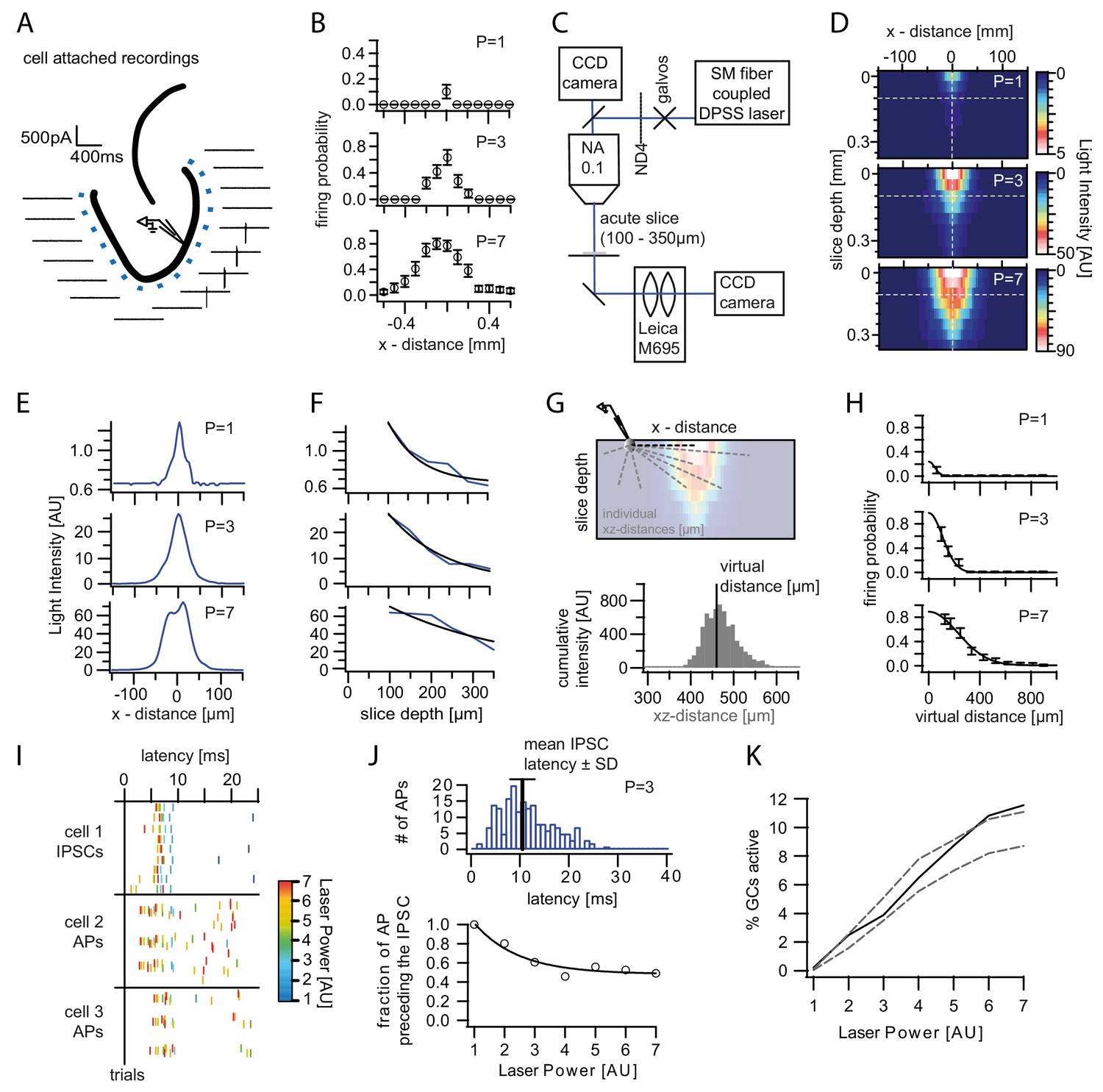
(A) Schematic illustration of the experimental setup. Cells were recorded in cell attached mode (two per slice), while systematically stimulating at varying distances. Traces from a representative trial at p=3. (B) Mean firing probability of every location over trials and cells for each laser power (three example powers shown). (C) Schematic of the modified setup to record the three dimensional light intensity profile in an acute slice. In order to avoid saturation a neutral density filter (ND4) was inserted into the light path. (D) Cross-section of the light intensity profile of the laser spot at increasing slice depth. The dashed white lines indicate the location of the cross sections shown in (E) and (F). Depths below 100 µm were extrapolated from fits to (E) and (F). (G) Top, Illustration of the calculation of the virtual distance for a particular cell/pixel 440 µm lateral to the laser focus. The distances between the given cell/pixel and all other pixels (individual xz-distances) were weighted by the intensity at those pixels. Bottom, this weighting is illustrated by a histogram displaying the intensities for each respective xz-distance. The virtual distance corresponds to the intensity weighted mean of xz-distances. (H) The measured firing probabilities were assigned to the respective virtual distances. The resulting firing probability distribution was well approximated by a Gaussian fit (black lines). (I) Example of the IPSC and AP latencies upon a stimulation pulse from an individual slice. Laser Powers are color coded. (J) Top, Example Histogram of the distribution of all AP latencies for p=3 (blue). The black bar indicates the mean IPSC latency ± standard deviation at that power. Bottom, The fraction of action potentials that precede the mean IPSC for each power was well approximated by an exponential fit (black line). Light stimulation in (I) and (J) was from 0 to 20 ms. (K, black) Estimated active cell fraction in the slice calculated from the light intensity profiles in (D) and the virtual firing probability distributions in (H) and corrected by the fraction of APs occurring after the mean IPSC (J). The estimated active cell fraction is identical to the mean firing probability throughout the slice. For comparison, the cell fraction was also estimated assuming no firing probability decay with increasing depth (upper grey dashed line) or assuming isometric decay (lower grey dashed line).
Figure 2—figure supplement 2
Error in somatic IPSC measurements with increasing inhibitory conductance.
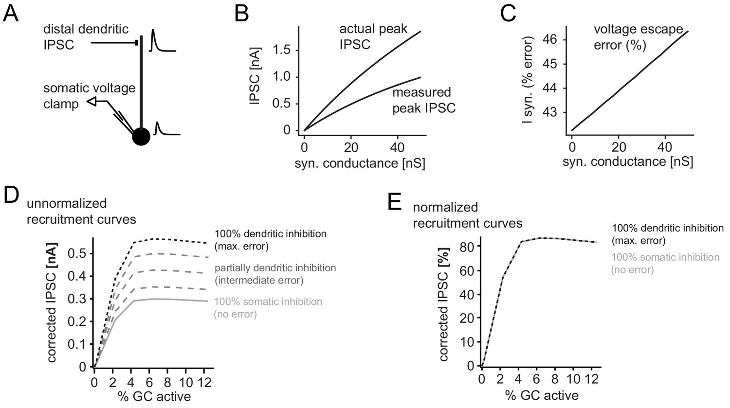
A simple ball and stick model was used to estimate the impact of voltage escape errors for dendritic IPSCs (soma diameter 20um; dendrite diameter and length 3 µm and 200 µm, respectively). To estimate the maximum errors the inhibitory synapse was placed at a distal site (180 µm from the soma) and inhibitory currents were measured using a single electrode voltage-clamp at the soma. (A) Illustration of the model and an attenuated somatic IPSC measurement. (B) Peak amplitudes of the measured IPSC over a range of distal synaptic conductances (measured peak IPSC), as well as the actual peak IPSC in the absence of voltage errors, calculated from the transfer and input impedances of the model. (C) Error in somatically measured peak IPSC as percentage of the actual peak IPSC (I syn, % error) at a given synaptic conductance. Errors in estimating synaptic inhibitory currents were linear. (D) Illustration of corrected and uncorrected recruitment curves of absolute IPSC amplitudes for varying degrees of voltage error (using data from the recruitment curve in Figure 2H). Note that due to the linearity of voltage escape errors, absolute IPSC amplitudes change, but the saturation point does not. (E) This is illustrated by the normalized recruitment curves, as shown throughout the manuscript (see Figure 2H). Note that normalized curves are practically unaffected by voltage escape errors.
Figure 2—figure supplement 3

Absence of single GC induced feedback inhibition.
Pairs of juxtaposed GCs (<100 µm distance) were recorded to test for single GC induced feedback inhibition. (A) Schematic illustration of the experimental setup. (B) Example of a paired recording where cell one is fired at 100 Hz in current clamp mode while cell two is recorded in voltage clamp mode in order to detect IPSCs. (gray, 10 individual trials; black, average).
Figure 3
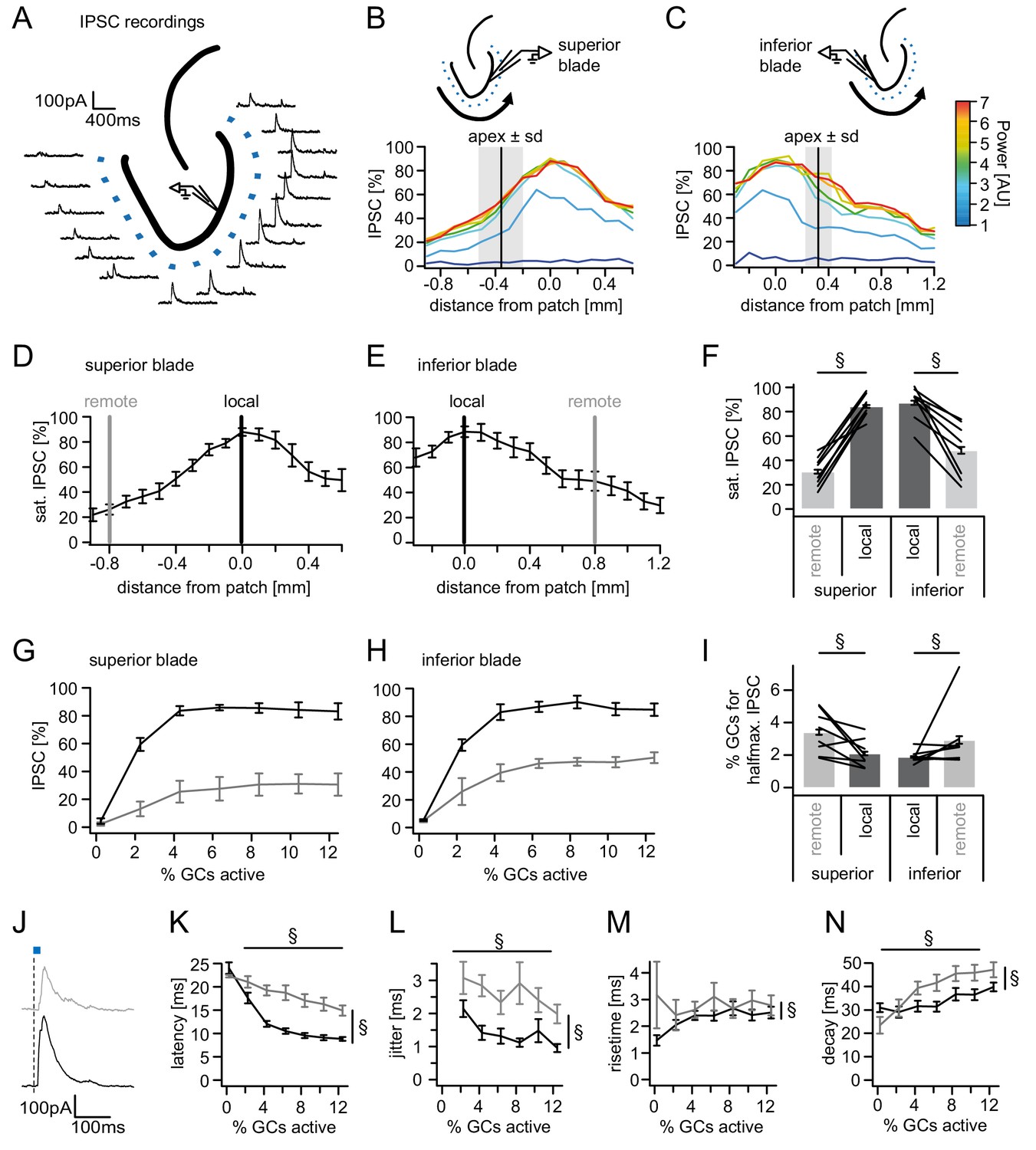
Spatial organization of feedback inhibition.
Feedback IPSCs recorded from an individual GC while GCs at varying distances were activated. (A) Schematic illustration of the stimulation paradigm and example IPSC traces of an individual trial (p=3). (B, C) Distribution of normalized IPSC amplitudes as a function of laser power and distance from stimulation spot for superior and inferior blade GCs (n = 8 for each blade). The relative location of the DG apex ± standard deviation is indicated by the black bar and grey area respectively. (D, E) IPSC distribution over space at saturation (p≥5). Black and grey bars indicate a local and a remote location at 800 µm from the recorded cell respectively. (F) Comparison of the amplitude of the locally and remotely activated IPSCs at saturation (two-way RM ANOVA, overall test significance indicated by §). (G, H) Comparison of the recruitment curves during local (black) or remote (grey) stimulation for superior and inferior blade respectively. (I) Comparison of the cell fraction required for halfmaximal IPSC activation between stimulation sites and blades (two-way RM ANOVA overall test significance indicated by §). (J–M) Temporal properties of IPSCs between local (black) and remote (grey) stimulation. To test for systematic variations of kinetic parameters with increasing active cell fractions as well as stimulation site two-way RM ANOVAs with no post tests were performed. Overall significance indicated by §. (K) Latency from beginning of light pulse to IPSC (L) temporal jitter of IPSCs (SD of latency within cells) (M) 20% to 80% rise time (N) IPSC decay time constant.
Figure 4 with 1 supplement
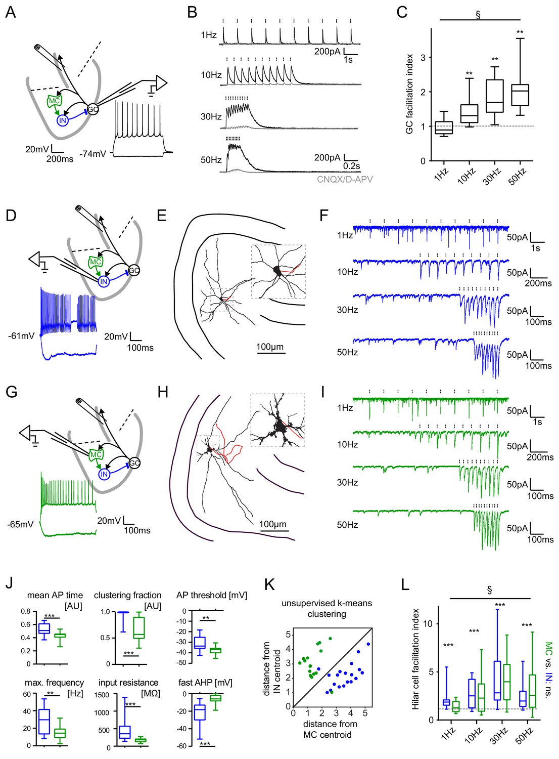
Short-term dynamics in the feedback inhibitory microcircuit.
Trains of ten antidromic electrical stimulations at 1, 10, 30 or 50 Hz were applied to elicit disynaptic feedback inhibition or excitation of hilar cells (electrical stimulation artifacts were removed in all traces). (A, D, G) Schematic illustration of the experimental setup and example traces of voltage responses to positive and negative current injections of GC and hilar cells (dashed lines indicate cuts to sever CA3 backprojections). (B) Exemplary GC feedback IPSCs before (black) and after (grey) glutamatergic block (n = 7). (C) Facilitation indices (mean of the last three IPSCs normalized to the first; n = 10 cells). (D-L) Hilar cells were manually classified into putative interneurons (blue) or mossy cells (green) based on their morpho-functional properties. (E) Reconstruction of biocytin filled hilar interneuron (axon in red). (F) Interneuron EPSCs in response to stimulation trains. (H) Reconstruction of biocytin filled mossy cell (axon in red). (I) Mossy cell EPSCs in response to stimulation trains. (J) Quantification of intrinsic properties of hilar cells (see Materials and methods). (K) k-means clustering based on intrinsic properties of hilar cells (coloring according to manual classification). (L) Facilitation indices of classified hilar cells. (§ indicates significance in one-way RM ANOVA, * show significance in Bonferroni corrected Wilcoxon signed rank tests for deviation from 1).
Figure 4—figure supplement 1

Frequency dependence of feedback inhibition over space.
Trains of 10 focal optic stimulations (20 ms duration) were applied either locally (1) or remotely (2) to elicit feedback inhibition. (A) Schematic of the experimental paradigm and example traces of elicited cell attached spikes or IPSCs. (B) Example traces for stimulation at 1, 10, 30 Hz or continuously for 200 ms of a local or remote GC populations (black and grey, respectively). (C) The AP probability index (mean probability during the last three pulses normalized to the first pulse (one-way RM ANOVA, p < 0.001 for frequency, Bonferroni corrected Wilcoxon signed rank test for deviation from 1; p = 0.024, = 0.008, = 0.008 and = 0.008 for 1 Hz, 10 Hz, 30 Hz and continuous stimulation, respectively). (D) Facilitation indices of local (dark grey) and remote (light grey) stimulation (two-way RM ANOVA; p = 0.635, = 0.314 and = 0.687 for location, frequency and interaction, respectively).
Figure 5 with 1 supplement
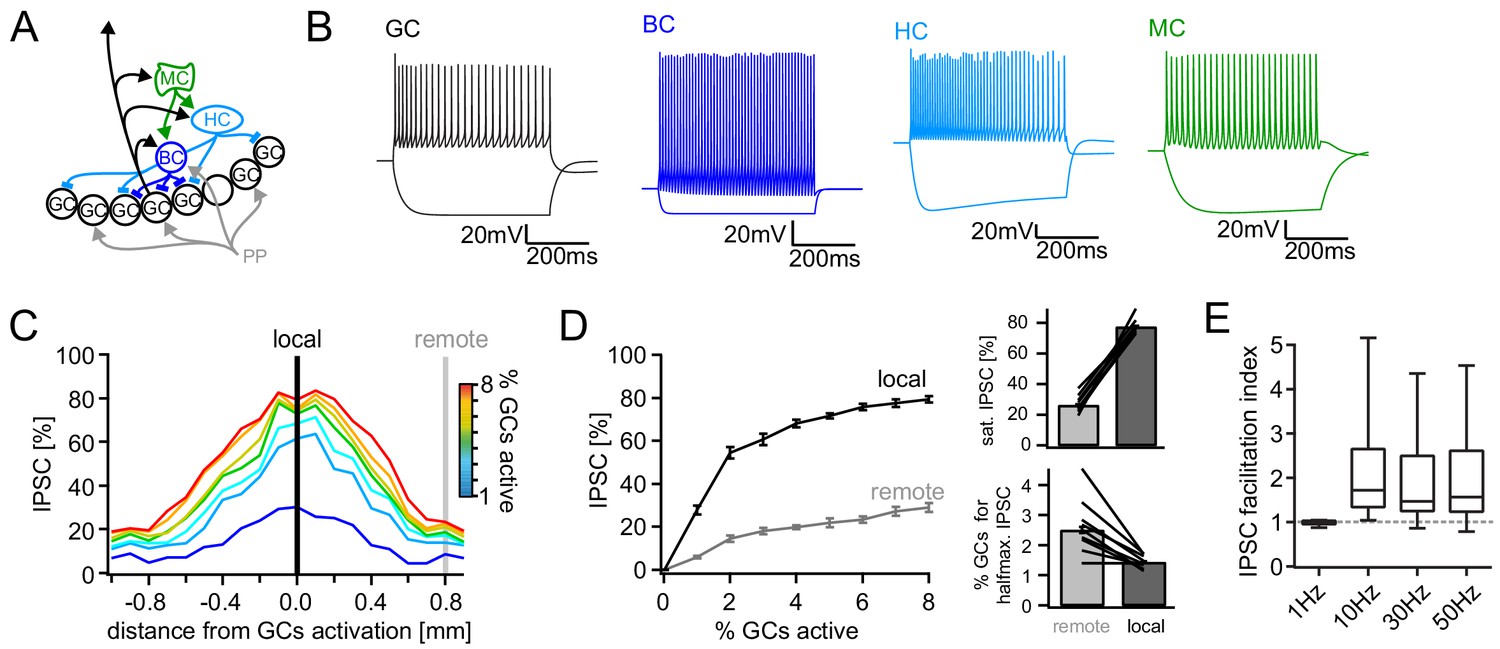
Computational model of the DG feedback circuit.
A biophysically realistic model of DG was tuned to capture the key quantitative features of the feedback circuit. All analyses were performed as for the real data (including IPSC normalization to maximal IPSC over space and power within each respective cell) (A) Schematic of the model circuit. GC: granule cell, BC: basket cell, HC: hilar perforant path associated cell, MC; mossy cell. (B) Intrinsic responses of model cell types to positive and negative current injections. (C) Spatially graded net feedback inhibition following simulated focal GC activation. (D) Local and remote recruitment curves of the feedback inhibitory circuit (left) and the resulting saturated IPSC amplitudes and GC fractions recruiting halfmaximal inhibition (right). (E) Facilitation indices resulting from simulated, 10 pulse, frequency stimulation of GCs as above.
Figure 5—figure supplement 1
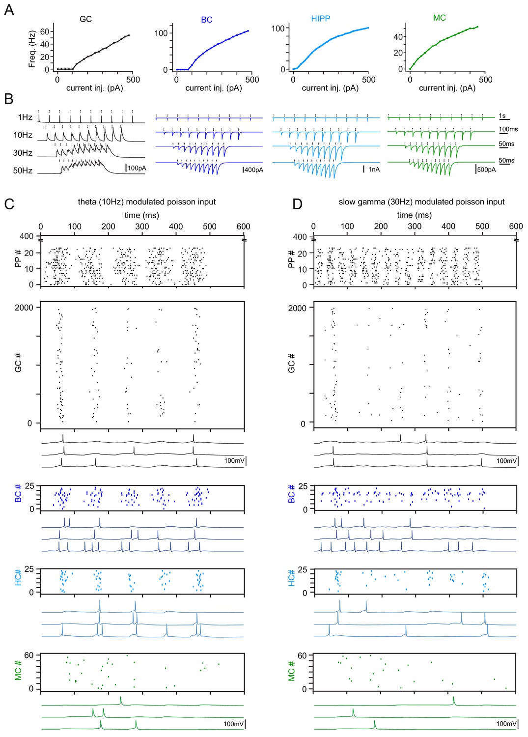
Model tuning and validation.
(A) Frequency responses to somatic current injections of model cell types (GC: granule cells, BC: basket cells, HC: hilar perforant path associated cells, MC: mossy cells). All model cells were matched to data by Santhakumar et al. (2005). (B) Simulation of synchronous frequency stimulation of GCs and the resulting PSCs in modeled cell types, analogous to Figure 4. (C) Representative theta modulated PP input and population responses (scatterplots) of all modeled cell types. Following each scatterplot are three examples of spiking cells of the respective type. (D) Same as (C) but for slow gamma modulated inputs.
Figure 6 with 7 supplements

Frequency dependent pattern separation of temporally structured inputs.
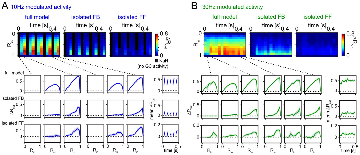
The quantitative DG model was challenged with theta (10 Hz) or slow gamma (30 Hz) modulated input patterns with defined overlap to probe its pattern separation ability. (A) Pair of theta modulated perforant path input patterns in which 50% of afferents overlap (grey area). (B) Resulting pair of GC output patterns of the full tuned network. Bottom: Representative individual GC underlying the observed patterns. (C) Comparison of 325 input pattern pairs and their resulting output pattern pairs. Each pair is characterized by its rate vector correlation for inputs (Rin) and outputs (Rout), where rates are measured over the full 600 ms time window. Dashed black lines represent the bin-wise mean Rout (in Rin bins of 0.1). Left: full tuned model, middle: model without mossy fiber inputs to interneurons, right: model without inhibitory synapses. (D) Full pattern separation effects (mean ΔRout) of all three conditions for both frequency domains quantified as the area enclosed by the dashed and unity lines in (C). Black lines represent individual network seeds. Two-way RM ANOVA indicated significance of condition, frequency and interaction, * indicate significance in Sidak’s posttests between individual conditions. (E) Isolated effects of feedback and feedforward motifs obtained by pairwise subtraction of Rout between conditions for each individual comparison. The inset shows the resulting ΔRout for each Rin bin. The area under the curve quantifies the mean ΔRout as in (D). Two-way RM ANOVA indicated significance of condition, frequency and interaction. *** indicate p<0.001 in Sidak’s posttest. (F). 100 ms time-resolved pattern separation effects of the full model, isolated FB or FF inhibition for theta modulated input (10 Hz). All analyses were performed as above but with rate vector correlations computed for 100 ms time windows. The bottom insets show ΔRout as a function of input similarity for each time window. The bottom right insets show the evolution of the mean ΔRout over time. (G) Same as (F) but for slow gamma (30 Hz) modulated inputs. Arrow indicate the region of selectively increased pattern separation. Data in D-G represent mean ± SEM of n = 7 random network seeds.
Figure 6—figure supplement 1
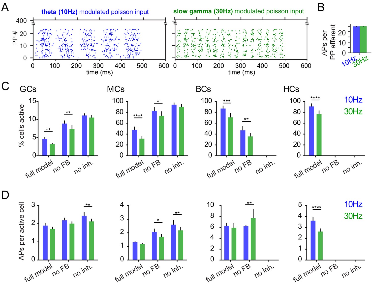
Activity levels and pattern separation.
(GCs: granule cells; MCs: mossy cells; BCs: basket cells; HCs: HIPP cells; n = 7 model runs). (A) Exemplary raster plots of 10 Hz and 30 Hz modulated inputs. (B) Mean number of action potentials per active perforant path afferent. (C) Percentages of active cells within the model. (D) Mean number of action potentials per active cell within the model. Activity rates (A, B) were tested with two-way ANOVAs followed by Sidak’s posttests for differences between frequencies. Asterisks indicate significance in posttests given significant overall effects (*p<0.05, **p<0.01, ***p<0.001, ****p<0.0001).
Figure 6—figure supplement 2
Robustness over different Similarity Metrics.
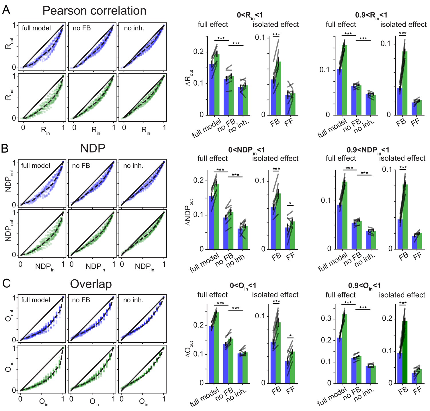
To test if the main finding of frequency dependent pattern separation, particularly for highly similar inputs, depended on the similarity metric used, the original data was reanalyzed with two alternative similarity metrics. As in the main figures data points in bar graphs represent the seven independent network seeds. For each network (seed), we ran sets of patterns for the full model, a network without feedback inhibition (no FB) and a model with no inhibition (no inh.). (A) Pearson’s correlation coefficient R (as in Figure 6) left: exemplary scatterplots of pattern separation effects. right: bargraphs of the mean pattern separation effect over the full input similarity range (0 < Rin1) or only highly similar input patterns (0.9 < Rin < 1). Full effects measure the mean pattern separation effect for each network condition: full model, no feedback (no FB) and no inhibition (no inh.). Isolated effects measure the pattern separation contribution of individual circuit motifs: feedback inhibition (FB) and feedforward inhibition (FF). (B) Same as (A) but using normalized dot product (NDP) as similarity metric for input and output comparisons. (C) Same as (A) but using population overlap as similarity metric. Overlap is defined as the number of cells active in both patterns (logical and) divided by the number of cells active in either pattern (logical or). The full effects were tested with 2 × 3 ANOVAs followed by Sidak’s posttests for differences between conditions. Isolated effects were tested with 2 × 2 ANOVAs followed by Tukey posttests for differences between frequencies. Asterisks indicate significance in posttests given significant overall effects (*p<0.05,**p<0.01,***p<0.001).
Figure 6—figure supplement 3
Isolated pattern separation effects of spatial tuning and MF facilitation.
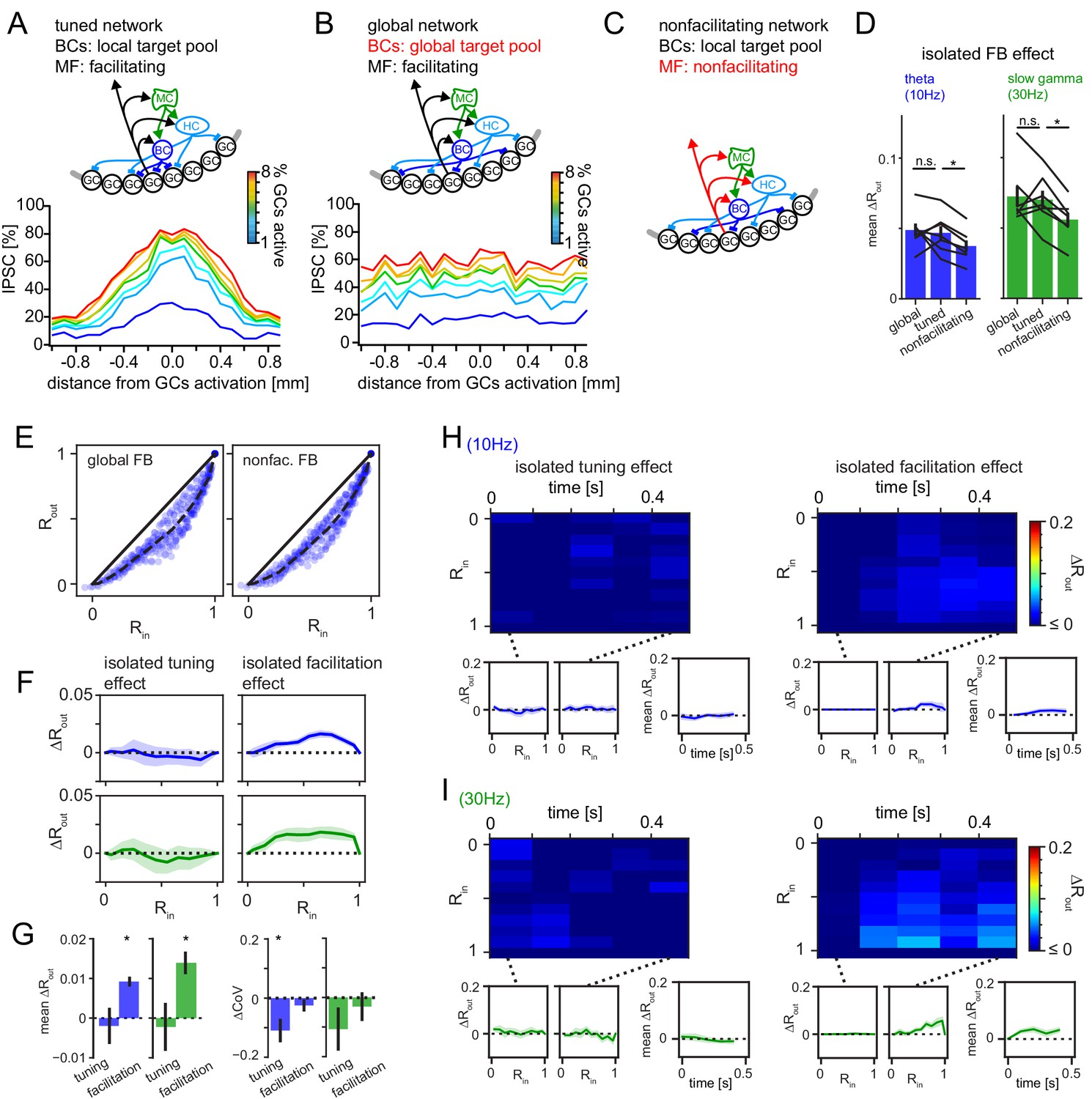
Effects of isolated manipulations were computed for the DG model as in Figure 6. (A) Schematic of the full tuned network and the resulting spatial profile of inhibition (as in Figure 5). (B) Schematic of the global network (with unrestricted BC target pool) and the resulting spatial profile of inhibition. (C) Schematic of the non-facilitating network. (D) Isolated mean feedback effects of the global, tuned and non-facilitating models. Two-way RM ANOVA showed: p < 0.001, = 0.020, = 0.402 for frequency, condition and interaction respectively with * indicating significance in Dunnett’s posttest against the full tuned effect. p = 0.742 and 0.020 for global and non-facilitating, respectively at 10 Hz; p = 0.650 and 0.001 for global and non-facilitating, respectively at 30 Hz. (E) Exemplary pattern separation plots of theta modulated inputs when spatial tuning (left) or MF facilitation (right) was removed. (F) Isolated pattern separation effects of the given manipulation for theta (blue) or gamma (green) modulated inputs as a function of input similarity. (G) Isolated effect of the given manipulation on mean ΔRout (left) and the coefficient of variance (ΔCoV) of pattern separation between individual comparisons (right). (H, I) Time-resolved analyses of isolated effects of spatial tuning (left) and MF facilitation (right) for theta (top row) and slow gamma (bottom row) modulated inputs. In each subpanel, the bottom left and middle insets show ΔRout as a function of input similarity of the first and last time windows respectively. The bottom right insets show the evolution of the mean ΔRout over time.
Figure 6—figure supplement 4
Robustness for shorter analysis time-window.
(A) 33 ms time-resolved pattern separation effects of the full model, isolated feedback (FB) or feedforward (FF) inhibition for theta modulated input (10 Hz). All analyses were performed as above but with rate vector correlations computed for 33 ms time windows (instead of 100 ms or 600 ms, as in Figure 6). The bottom insets show ΔRout as a function of input similarity for the first and last three time windows. The bottom right insets show the evolution of the mean ΔRout over time. (B) Same as (A) but for slow gamma (30 Hz) modulated inputs. Data represent mean ± SEM of n = 7 random network seeds.
Figure 6—figure supplement 5
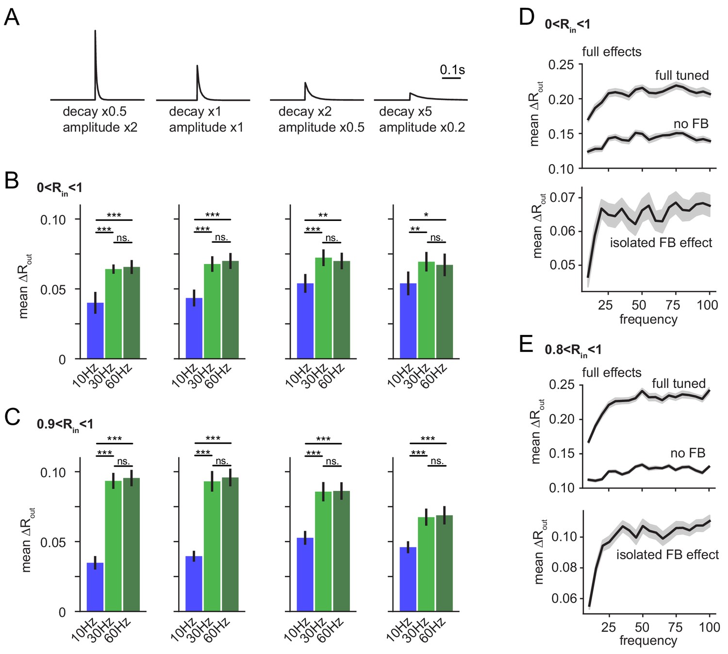
Robustness over various IPSC decay time-constants and over the full gamma range.
(A–C) To test if the frequency dependence of feedback inhibitory pattern separation remained robust for different IPSC decay time constants we probed a range of altered time constants (our experimentally matched time constant x0.5, x1, x2 and x5) while maintaining total inhibitory conductance in the network constant by complementary adjustment of IPSC amplitude. As we expected a potential interaction between IPSC decay and modulation frequency, we probed model runs for each factor with 10 Hz, 30 Hz and 60 Hz modulation. The isolated feedback inhibitory effects were computed and impacts of decay and frequency were examined with 4 × 3 ANOVAs followed by Tukey posttests for differences between frequencies. Asterisks indicate significance in posttests given significant overall effects (*p<0.05,**p<0.01,***p<0.001). (A) Illustration of modified IPSC time-courses. (B) Mean pattern separation effect of isolated feedback inhibition over the full input similarity range (0 < Rin < 1). (C) Same as (B) but only for highly similar input patterns. Analyses in A-C were performed on seven new network seeds with simulation and analysis otherwise identical to Figure 6. (D–E) To probe the robustness of frequency-dependent feedback inhibitory pattern separation over an even larger range of frequency modulation, we next simulated the effects over a range from 10 to 100 Hz in 5 Hz steps. To provide computational tractability, we performed only eight runs per frequency (instead of 24 runs as in all other simulations) leading to fewer pattern comparisons, and somewhat noisier readouts. For the majority of frequencies, no input comparisons with R > 0.9 occurred so we defined (0.8 < Rin < 1) as highly similar input patterns, potentially leading to a slight underestimation of our effects.
Figure 6—figure supplement 6
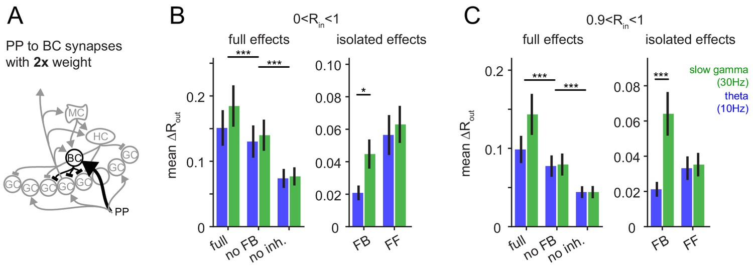
Robustness for increased feedforward inhibition.
To test if the frequency-dependent enhancement of feedback inhibitory pattern separation of highly similar inputs was sensitive to the changes in the relative strengths of feedforward and feedback inhibition, we increased the perforant path (PP) to basket cell (BC) synapse weight 2x. (A) Illustration of the network alteration. (B) The resulting full pattern separation effects (left) and isolated feedback (FB) and feedforward (FF) effects (right) as mean over all input similarities. (C) Same as (B) but only for highly similar input patters. Full effects were tested with 2 × 3 ANOVAs followed by Sidak’s postests for differences between conditions. Isolated effects were tested with 2 × 2 ANOVAs followed by Tukey posttests for differences between frequencies. Asterisks indicate significance in posttests given significant overall effects (*p<0.05,**p<0.01,***p<0.001).
Figure 6—figure supplement 7
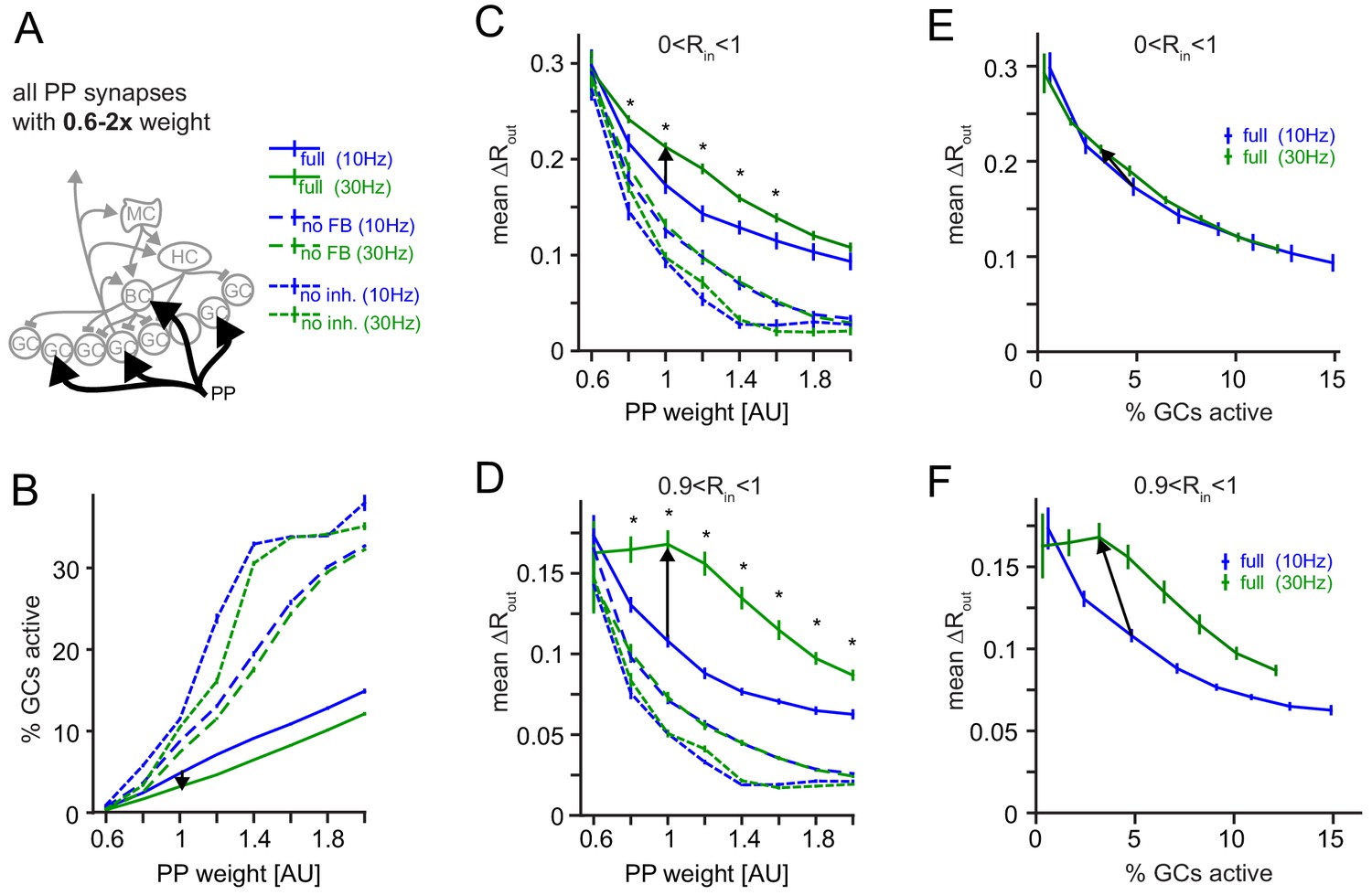
Robustness for increased perforant path (PP) drive.
The weight of the PP input synapses was varied between 0.6x to 2x their original weight. (A) Illustration of the network alteration. (B) Active GC fractions for the full network (full), the no feedback inhibition network (no FB) and the no inhibition network (no inh.), each for 10 and 30 Hz modulated PP input. The black arrow indicates the frequency effect for the default PP-weight (1x). (C) Full pattern separation effects over all input similarities (0 < Rin < 1). Asterisks indicate p<0.05 (uncorrected t-tests). (D) Full pattern separation effects for highly similar input patterns (0 < Rin < 1). Asterisks indicate p<0.05 (uncorrected t-tests). (E) Data for the full network from (B) and (C) plotted to show pattern separation as a function of GC sparsity. The arrow represents the default PP input strength. (F) Same as E, but only for highly similar input patterns.
Tables
Key resources table
| Reagent type (species) or resource | Designation | Source or reference | Identifiers | Additional information |
|---|---|---|---|---|
| Strain, strain background (Mus musculus) | C57BL/6N | Charles River | Strain Code 027 | |
| Strain, strain background (Mus musculus) | Prox1-Cre | MMRRC-UCD | RRID: MMRRC_036632-UCD | obtained as cryopreserved sperm and rederived in the local facility |
| Strain, strain background (Mus musculus) | Ai32-ChR-eYFP | Jackson Laboratory | RRID: IMSR_JAX:012569 | |
| Other | UGA-40 | RAPP Optoelectronics | Galvanometric, focal laser stimulation device | |
| Software, algorithm | Igor Pro 6.3 | Wavemetrics | ||
| Software, algorithm | Python 3.5 scikit learn | Pedregosa et al. (2011) | https://scikit-learn.org/stable/ | |
| Software, algorithm | ouropy | Custom Python code. This Paper | https://github.com/danielmk/ouropy | |
| Software, algorithm | pyDentate | Custom Python code, This Paper | https://github.com/danielmk/pyDentateeLife2020 | |
| Software, algorithm | Neuron 7.4 | Carnevale and Hines, 2006 | ||
| Software, algorithm | Prism 6 | Graphpad |
Additional files
-
Supplementary file 1
Literature review for DG circuit short-term dynamics.
Studies reporting short-term dynamics within the DG circuit were reviewed with a main focus on facilitation or depression of synaptic connections defined by pre and postsynaptic cell types. Note the abundance of depressing synapses (quantitative descriptions of depression blue). Also note the complexity of direct connections between Interneurons (lower third of the table).
- https://cdn.elifesciences.org/articles/53148/elife-53148-supp1-v1.xlsx
-
Supplementary file 2
Model parameters.
Overview of synaptic and intrinsic parameters between model cell-types. First row includes modeled cell number per type. PP: perforant path, GC: granule cell, MC: mossy cell, BC: basket cell, HC: Hilar perforant path associated cell; Weight: maximal synaptic conductance, Facilitation Max.: maximal fold increase of synaptic conductance, Decay Tau: synaptic decay time constant, Facilit. Tau: facilitation time constant, Delay: latency to postsynaptic event after presynaptic action potential, Target pool: range of n closest cells potentially receiving an output, Divergence: number of output synapses per cell stochastically picked from target pool, Target segments: cellular compartment receiving the synapse. Values in brackets are values for robustness analyses in Figs. S10, S11.
- https://cdn.elifesciences.org/articles/53148/elife-53148-supp2-v1.xlsx
-
Transparent reporting form
- https://cdn.elifesciences.org/articles/53148/elife-53148-transrepform-v1.pdf
Download links
A two-part list of links to download the article, or parts of the article, in various formats.
Downloads (link to download the article as PDF)
Open citations (links to open the citations from this article in various online reference manager services)
Cite this article (links to download the citations from this article in formats compatible with various reference manager tools)
Quantitative properties of a feedback circuit predict frequency-dependent pattern separation
eLife 9:e53148.
https://doi.org/10.7554/eLife.53148


