Neural dynamics of perceptual inference and its reversal during imagery
- Donders Centre for Cognition, Radboud University, Donders Institute for Brain, Cognition and Behaviour, Netherlands
- Wellcome Centre for Human Neuroimaging, University College London, United Kingdom
- Oxford Centre for Human Brain Activity, Oxford University, United Kingdom
- Department of Clinical Health, Aarhus University, Denmark
Figures
Figure 1
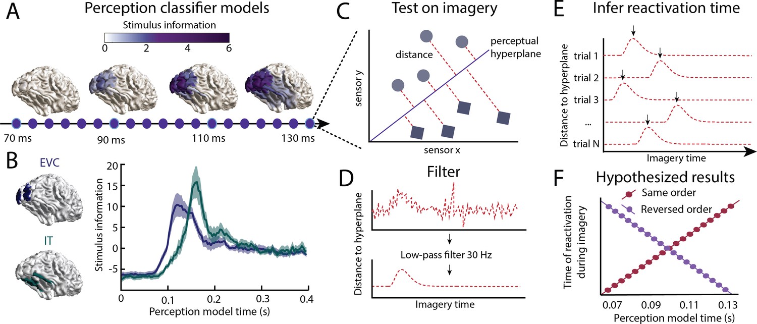
Inferring information flow using perceptual feed-forward classifier models.
(A–B) Perception models. At each point in time between 70 and 130 ms after stimulus onset, a perception model (classifier) was estimated using Linear Discriminant Analysis (LDA) on the activation patterns over sensors. (A) The source-reconstructed difference in activation between faces and houses (i.e. decoding weights or stimulus information) is shown for different time points during perception. (B) Stimulus information standardised over time is shown for low-level early visual cortex (EVC: blue) and high-level inferior temporal cortex (IT: green). These data confirm a feed-forward flow during the initial stages of perception. (C) Imagery reactivation. For each trial and time point during imagery, the distance to the perceptual hyperplane of each perception model is calculated. (D) To remove high-frequency noise, a low-pass filter is applied to the distance measured. (E) The timing of the reactivation of each perception model during imagery is determined by finding the peak distance for each trial. (F) Hypothesised results. This procedure results in a measure of the imagery reactivation time for each trial, for each perception model time point. If perception models are reactivated in the same order during imagery, there would be a positive relation between reactivation imagery time and perception model time. If instead, perception models are reactivated in reverse order, there would be a negative relation. Source data associated with this figure can be found in the Figure 1—source data 1 and 2.
-
Figure 1—source data 1
Source data for panel A.
Cfg = a configuration structure with the analysis options. Source = a FieldTrip source-reconstruction structure with the source-reconstructed stimulus information averaged over participants in the field source.avg.pow2. Bnd = the vertices which can be used to plot source-activation as ft_plot_mesh(bnd,. . . ).
- https://cdn.elifesciences.org/articles/53588/elife-53588-fig1-data1-v1.mat
-
Figure 1—source data 2
Source data for panel B.
Activation = subject x area x time source-reconstructed stimulus information.
- https://cdn.elifesciences.org/articles/53588/elife-53588-fig1-data2-v1.mat
Figure 2
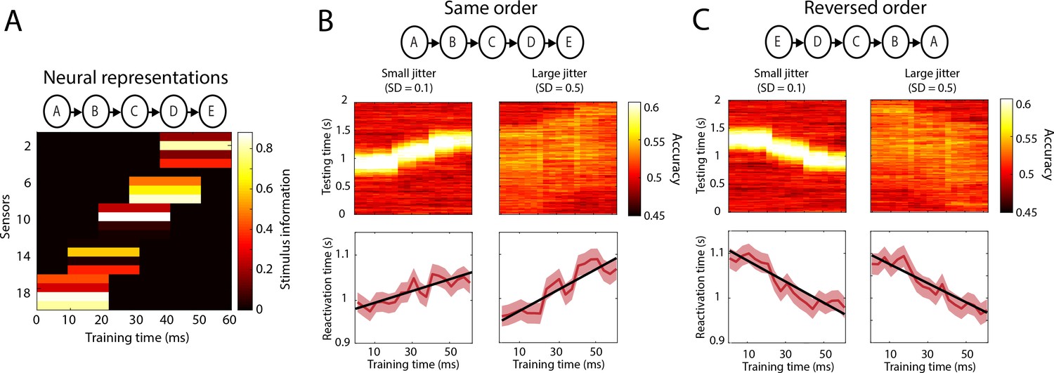
Simulations reactivation analysis.
(A) Five different neural representations, activated sequentially over time, were modelled as separate sensor activation patterns. Stimulus information is defined as the difference in activation between the two classes (i.e. what is picked up by the classifier). Results on a testing data-set in which the order of activation was either the same (B) or reversed (C). Top panels: cross-decoding accuracy obtained by averaging over trials. Bottom panels: reactivation times inferred per trial. Source data associated with this figure can be found in the Figure 2—source data 1.
-
Figure 2—source data 1
Source data from the simulations.
jitSD_vals = the SD values used to create the between-trial jitter of the different data sets. models = senors x perception time points x stimulus classes activation patterns. accSO = per jitter value a cell containing nsubjects x perception training time points x imagery testing points decoding accuracy for a dataset in which reactivation happened in the same order. accRO = same for reactivation in reversed order. reactSO = per jitter value a cell containing nsubjects x ntrials x perception training time points reactivation times for a dataset in which reactivation happened in the same order. reactRO = same for reactivation in reversed order.
- https://cdn.elifesciences.org/articles/53588/elife-53588-fig2-data1-v1.mat
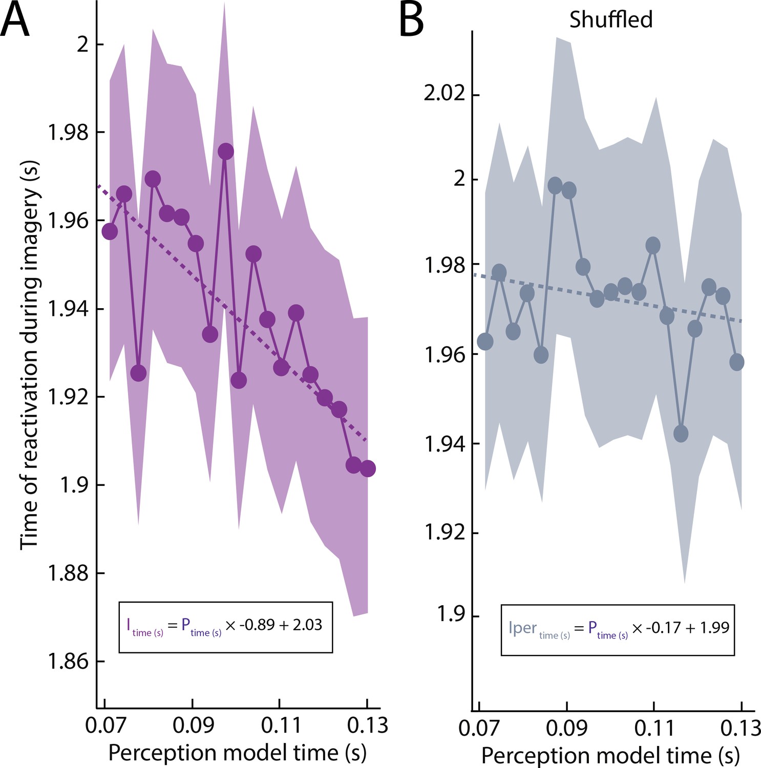
Figure 3 with 1 supplement
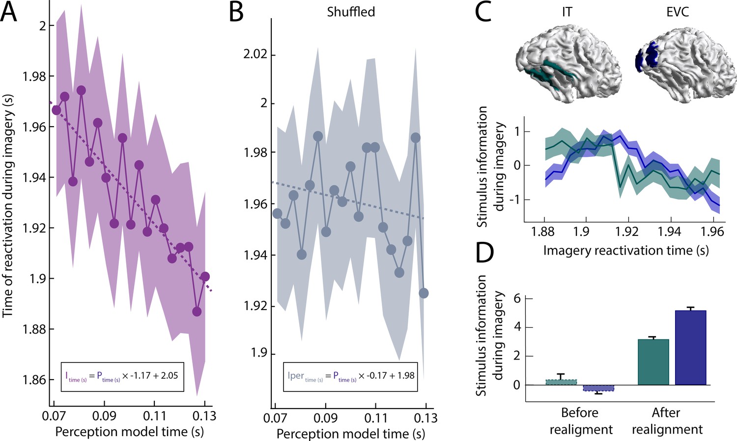
Imagery reactivation results.
(A) Reactivation time during imagery for every perception model averaged over trials. The shaded area represents the 95% confidence interval. The linear equation shows how imagery reactivation time (I) can be calculated using perception model time (P) in seconds. (B) Same results after removing stimulus information by permuting the class-labels (C–D) Stimulus information during imagery was estimated by realigning the trials based on the reactivation time points and using the linear equation to estimate the imagery time axis. (C) Stimulus information standardised over time for low-level early visual cortex (EVC) and high-level inferior temporal cortex (IT). (D) Stimulus information in EVC and IT averaged over time before and after realignment. Stimulus information below 0 indicates that the amount of information did not exceed the permutation distribution. Source data associated with this figure can be found in the Figure 2—source data 1–6.
-
Figure 3—source data 1
Contains the reactivation time per perception model and per trial, the subject ID ('S').
- https://cdn.elifesciences.org/articles/53588/elife-53588-fig3-data1-v1.mat
-
Figure 3—source data 2
Contains the source-reconstructed stimulus information as subject x source parcel x time points as well as the corresponding time vector and source-parcel names for the realigned data.
- https://cdn.elifesciences.org/articles/53588/elife-53588-fig3-data2-v1.mat
-
Figure 3—source data 3
Contains the source-reconstructed stimulus information as subject x source parcel x time points as well as the corresponding time vector and source-parcel names for the unaligned data.
- https://cdn.elifesciences.org/articles/53588/elife-53588-fig3-data3-v1.mat
-
Figure 3—source data 4
Contains the reactivation time per perception model and per trial, the subject ID ('S') for the permuted classifier.
- https://cdn.elifesciences.org/articles/53588/elife-53588-fig3-data4-v1.mat
-
Figure 3—source data 5
Contains the reactivation time per perception model and per trial, the subject ID ('S') for the unfiltered data.
- https://cdn.elifesciences.org/articles/53588/elife-53588-fig3-data5-v1.mat
-
Figure 3—source data 6
Contains the reactivation time per perception model and per trial, the subject ID ('S') for the unfiltered and permuted data.
- https://cdn.elifesciences.org/articles/53588/elife-53588-fig3-data6-v1.mat
Figure 3—figure supplement 1
Imagery reactivation results without the low-pass filter.
(A) Unpermuted data. (B) Permuted data.
Figure 4 with 3 supplements
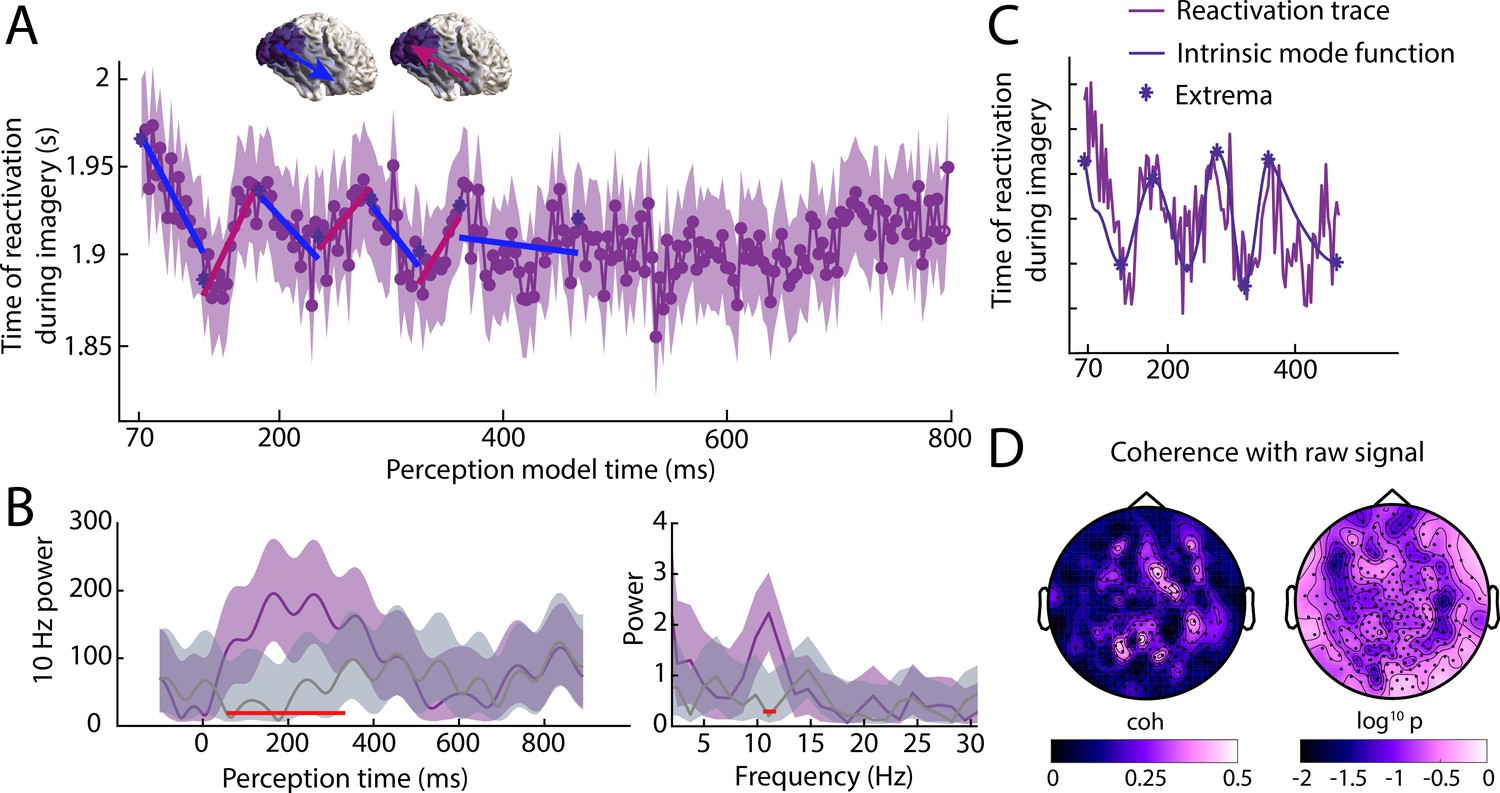
Reactivation timing during imagery for classifiers trained at all perception time points.
(A) Imagery reactivation time for perception models trained on all time points. On the x-axis the training time point during perception is shown and on the y-axis the reactivation time during imagery is shown. The dots represent the mean over trials for individual time points and the shaded area represents the 95% confidence interval. (B) Left: time-frequency decomposition using a Morlet wavelet at 10 Hz. Right: power at different frequencies using a Fast Fourier Transformation. The purple line represents the true data and the grey line represents the results from the shuffled classifier. Shaded areas represent 95% confidence intervals over trials. Red lines indicate time points for which the true and shuffled curve differed significantly (FDR corrected). (C) Intrinsic mode function and its extrema derived from the reactivation traces using empirical model decomposition. (D) Coherence between reactivation trace and raw signal. Left coherence values, right log10 p values. Source data associated with this figure can be found in the Figure 4—source data 1–3.
-
Figure 4—source data 1
Contains the identified reactivation trace extrema based on EMD of the empirical traces.
- https://cdn.elifesciences.org/articles/53588/elife-53588-fig4-data1-v1.mat
-
Figure 4—source data 2
Contains the reactivation traces as reactivation sample point per trial x perception model time for the unpermuted classifiers.
- https://cdn.elifesciences.org/articles/53588/elife-53588-fig4-data2-v1.mat
-
Figure 4—source data 3
Contains the reactivation traces as reactivation sample point per trial x perception model time for the permuted classifiers.
- https://cdn.elifesciences.org/articles/53588/elife-53588-fig4-data3-v1.mat
Figure 4—figure supplement 1

Reactivation timing during imagery for all perception time points without low-pass filter.
Figure 4—figure supplement 2
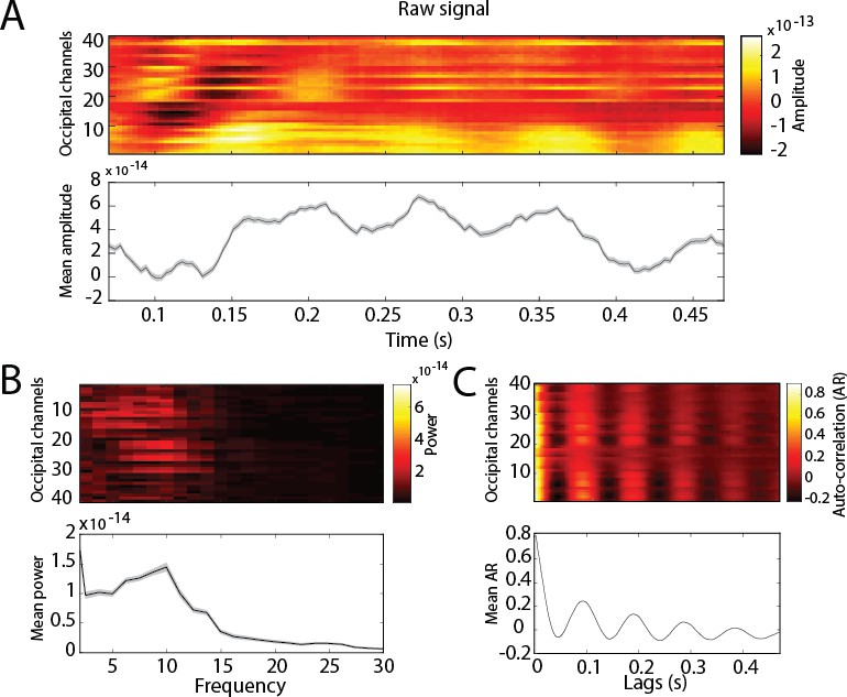
Dynamics of the raw signal during perception for occipital channels.
Top panels: per channel. Bottom panels: averaged over channels. Shaded area represents the 95% CI over trials. (A) Raw signal amplitude. (B) Frequency decomposition. (C) Auto-correlation.
Figure 4—figure supplement 3
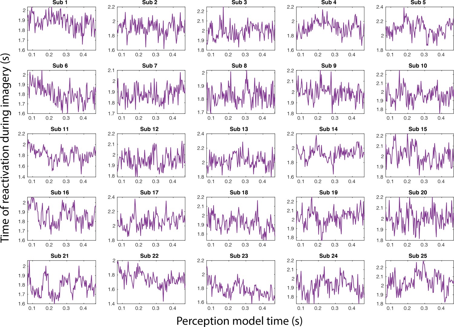
Imagery reactivation traces for the full perception period separately for each subject.
Figure 5
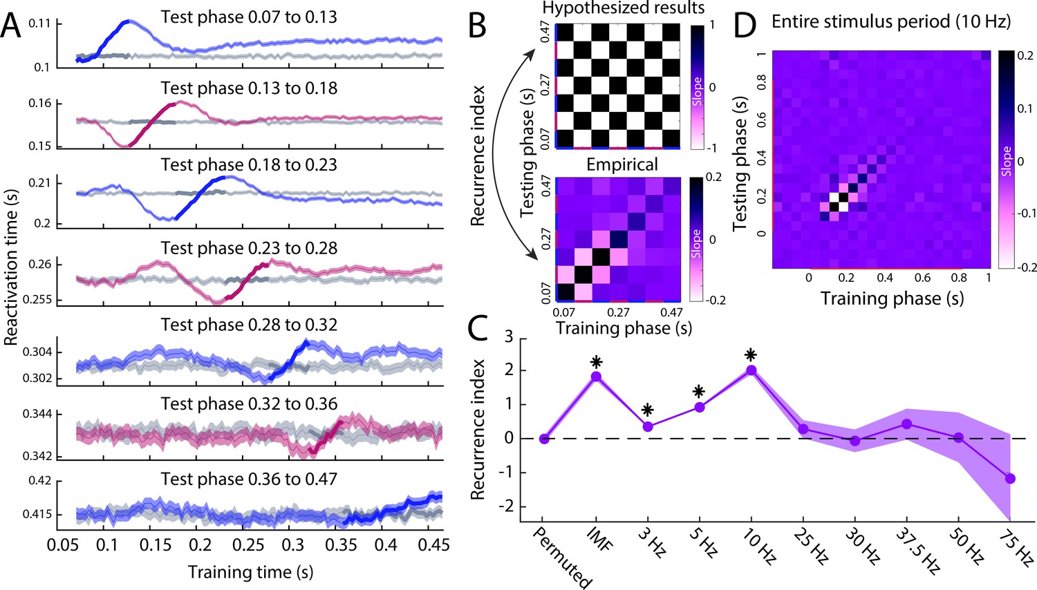
Reactivation timing for different perception phases.
(A) The reactivation traces for each testing phase. Blue traces reflect feed-forward phases, pink traces reflect feedback phases (Figure 4A) and grey traces reflect reactivation traces for permuted classifiers. Shaded area represents the 95% confidence interval over trials. (B) Hypothesised (top) and empirical (bottom) slopes between the training and testing phases. The hypothesised matrix assumes recurrent processing such that subsequent phases show a reversal in the direction of information flow. Recurrence index reflects the amount of recurrent processing in the data, which is quantified as the dot product between the vectorised hypothesis matrix and empirical matrix. (C) Recurrence index for the permuted classifier, phase specification based on the IMF of the imagery reactivation trace (Figure 4C) and phase specification on evoked oscillations at various frequencies. (D) Slope matrix for phase specification defined at 10 Hz over the entire stimulus period. Source data associated with this figure can be found in the Figure 5—source data 1–8.
-
Figure 5—source data 1
Contains, for the segmentation of 3 Hz, Cfg = a configuration structure with the analysis options.
S = per trial, the subject ID. L = for testing x training combination, the sample (time point) of maximum reactivation per trial. Btstrp = bootstrapping samples over trials per phase, per time point. Osc_btstrp = recurrence index calculated for each bootstrapping sample.
- https://cdn.elifesciences.org/articles/53588/elife-53588-fig5-data1-v1.mat
-
Figure 5—source data 2
Contains, for the segmentation of 5 Hz, Cfg = a configuration structure with the analysis options.
S = per trial, the subject ID. L = for testing x training combination, the sample (time point) of maximum reactivation per trial. Btstrp = bootstrapping samples over trials per phase, per time point. Osc_btstrp = recurrence index calculated for each bootstrapping sample.
- https://cdn.elifesciences.org/articles/53588/elife-53588-fig5-data2-v1.mat
-
Figure 5—source data 3
Contains, for the segmentation of 10 Hz, Cfg = a configuration structure with the analysis options.
S = per trial, the subject ID. L = for testing x training combination, the sample (time point) of maximum reactivation per trial. Btstrp = bootstrapping samples over trials per phase, per time point. Osc_btstrp = recurrence index calculated for each bootstrapping sample.
- https://cdn.elifesciences.org/articles/53588/elife-53588-fig5-data3-v1.mat
-
Figure 5—source data 4
Contains, for the segmentation of 25 Hz, Cfg = a configuration structure with the analysis options.
S = per trial, the subject ID. L = for testing x training combination, the sample (time point) of maximum reactivation per trial. Btstrp = bootstrapping samples over trials per phase, per time point. Osc_btstrp = recurrence index calculated for each bootstrapping sample.
- https://cdn.elifesciences.org/articles/53588/elife-53588-fig5-data4-v1.mat
-
Figure 5—source data 5
Contains, for the segmentation of 30 Hz, Cfg = a configuration structure with the analysis options.
S = per trial, the subject ID. L = for testing x training combination, the sample (time point) of maximum reactivation per trial. Btstrp = bootstrapping samples over trials per phase, per time point. Osc_btstrp = recurrence index calculated for each bootstrapping sample.
- https://cdn.elifesciences.org/articles/53588/elife-53588-fig5-data5-v1.mat
-
Figure 5—source data 6
Contains, for the segmentation of 37.5 Hz, Cfg = a configuration structure with the analysis options.
S = per trial, the subject ID. L = for testing x training combination, the sample (time point) of maximum reactivation per trial. Btstrp = bootstrapping samples over trials per phase, per time point. Osc_btstrp = recurrence index calculated for each bootstrapping sample.
- https://cdn.elifesciences.org/articles/53588/elife-53588-fig5-data6-v1.mat
-
Figure 5—source data 7
Contains, for the segmentation of 50 Hz, Cfg = a configuration structure with the analysis options.
S = per trial, the subject ID. L = for testing x training combination, the sample (time point) of maximum reactivation per trial. Btstrp = bootstrapping samples over trials per phase, per time point. Osc_btstrp = recurrence index calculated for each bootstrapping sample.
- https://cdn.elifesciences.org/articles/53588/elife-53588-fig5-data7-v1.mat
-
Figure 5—source data 8
Contains, for the segmentation of 75 Hz, Cfg = a configuration structure with the analysis options.
S = per trial, the subject ID. L = for testing x training combination, the sample (time point) of maximum reactivation per trial. Btstrp = bootstrapping samples over trials per phase, per time point. Osc_btstrp = recurrence index calculated for each bootstrapping sample.
- https://cdn.elifesciences.org/articles/53588/elife-53588-fig5-data8-v1.mat
Additional files
-
Supplementary file 1
Linear Mixed Model Bayesian Information Criterion (BIC) output for the different models.
(a) Bayesian Information Criterion (BIC) for linear mixed-effects model explaining imagery reactivation time with perception model time. (b) BIC for linear mixed-effects model explaining imagery reactivation time with perception model time after permuting the stimulus-class labels. (c) BIC for linear mixed-effects model explaining imagery reactivation time averaged over trials within subject with perception model time.
- https://cdn.elifesciences.org/articles/53588/elife-53588-supp1-v1.docx
-
Transparent reporting form
- https://cdn.elifesciences.org/articles/53588/elife-53588-transrepform-v1.docx
Download links
A two-part list of links to download the article, or parts of the article, in various formats.
Downloads (link to download the article as PDF)
Open citations (links to open the citations from this article in various online reference manager services)
Cite this article (links to download the citations from this article in formats compatible with various reference manager tools)
Neural dynamics of perceptual inference and its reversal during imagery
eLife 9:e53588.
https://doi.org/10.7554/eLife.53588


