The neurons that mistook a hat for a face
- Department of Psychology, University of Pennsylvania, United States
- Department of Neuroscience, Washington University in St. Louis, United States
- Department of Neurobiology, Harvard Medical School, United States
Figures
Figure 1 with 5 supplements
Experimental schematic and spatial selectivity of responsiveness.
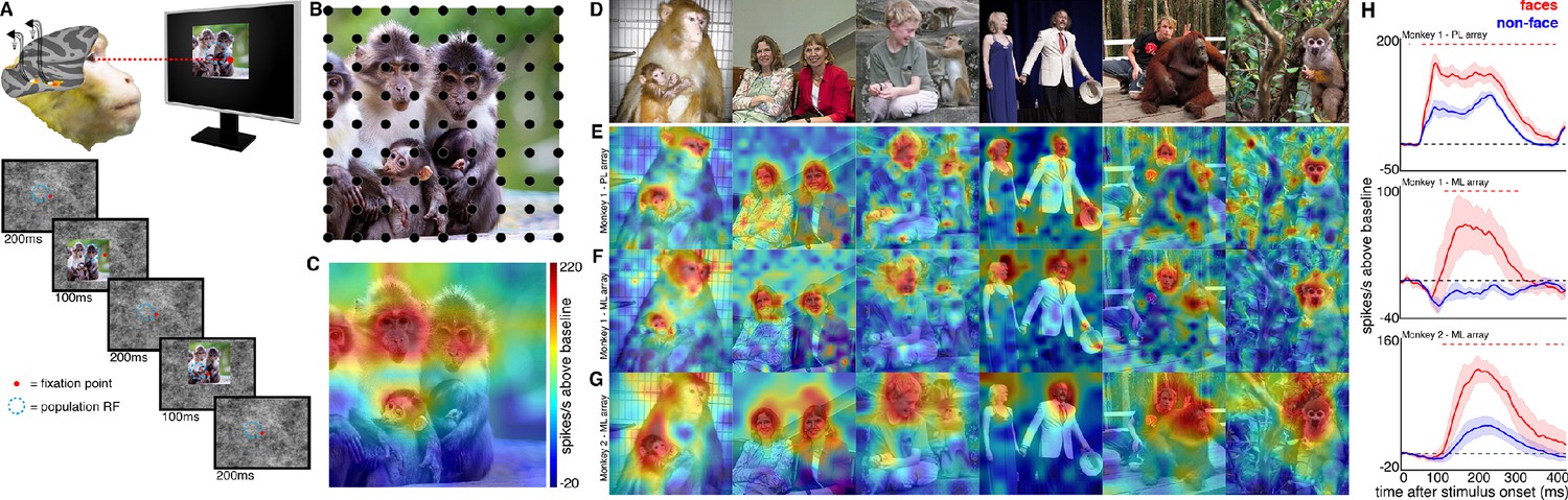
(A) The monkey maintains fixation (red spot) while a large (16° x 16°) complex natural scene is presented at locations randomly sampled from a 17 × 17 (Monkey 1) or 9 × 9 (Monkey 2) grid of positions centered on the array’s receptive field (blue dotted circle). On a given trial, 3 different images are presented sequentially at 3 different positions. Across the experiment, each image is presented multiple times at each position on the grid. (B) Parts of a 16° x 16° image (black dots) that were centered within each array’s receptive fields across trials from the 9 × 9 stimulus presentation grid; position spacing, 2°. (C) Map of a face cell’s firing rate (100–250 ms after stimulus onset) in response to different parts of the image positioned over the receptive field (recording site 15 in Monkey 1 ML array). The most effective parts of this image were the monkey faces. (D) Complex natural images shown to the monkey. Population-level response maps to these images from (E) PL in Monkey 1; (F) ML in Monkey 1; and (G) ML in Monkey 2. Firing rates were averaged over 100–250 ms post stimulus onset for Monkey 1 and 150–300 ms for Monkey 2. For E, F, and G, the color scale represents the range between 0.5% and 99.5% percentiles of the response values to each image. All 3 arrays showed spatially specific activation to the faces in the images, with higher selectivity in the middle face patches. (H) PSTHs of responses to face (red) and non-face (blue) parts of these images for (top) Monkey 1 PL, (middle) Monkey 1 ML, and (bottom) M2 ML. Shading represents 95% confidence limits. Dashed red lines denote time window with a significant difference in response magnitude between face and non-face image parts (paired t-test across 8 images; t(7) > 2.64; p<0.05, FDR-corrected).
© 2014 Patrick Bolger. All rights reserved. The image in Panel B is used with permission from Patrick Bolger@Dublin Zoo. It is not covered by the CC-BY 4.0 license and further reproduction of this panel would need permission from the copyright holder.
© 2009 Ralph Siegel. All rights reserved. The second photograph in Panel D is courtesy of Ralph Siegel. It is not covered by the CC-BY 4.0 license and further reproduction of this panel would need permission from the copyright holder.
© 2012 A Stubbs. All rights reserved. The fourth photograph in Panel D is courtesy of A Stubbs. It is not covered by the CC-BY 4.0 license and further reproduction of this panel would need permission from the copyright holder.
© 2008 Johnny Planet. All rights reserved. The fifth photograph in Panel D is courtesy of Johnny Planet. It is not covered by the CC-BY 4.0 license and further reproduction of this panel would need permission from the copyright holder.
Figure 1—figure supplement 1
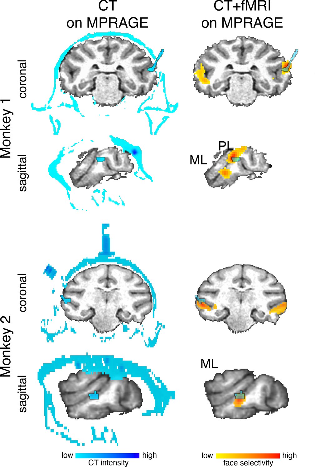
Localization of arrays.
Multi-electrode arrays were chronically implanted into two face patches within IT of two macaque monkeys. Arrays (outlined blue regions in the brain) were visualized with CT imaging. CT images were then rigidly aligned to a MPRAGE image of each monkey’s anatomy. (top) In Monkey 1, one Microprobes FMA array (blue outline) was implanted in the PL face patch. One NeuroNexus Matrix array was implanted in the ML face patch. This array was not visible on the CT image. (bottom) In Monkey 2, one Microprobes FMA array (outlined blue regions in the brain) was implanted in the ML face patch. Data threshold at t(2480) > 3.91 (p<0.0001 FDR-corrected) and t(1460) > 3.91 (p<0.0001 FDR-corrected) for monkeys 1 and 2, respectively.
Figure 1—figure supplement 2
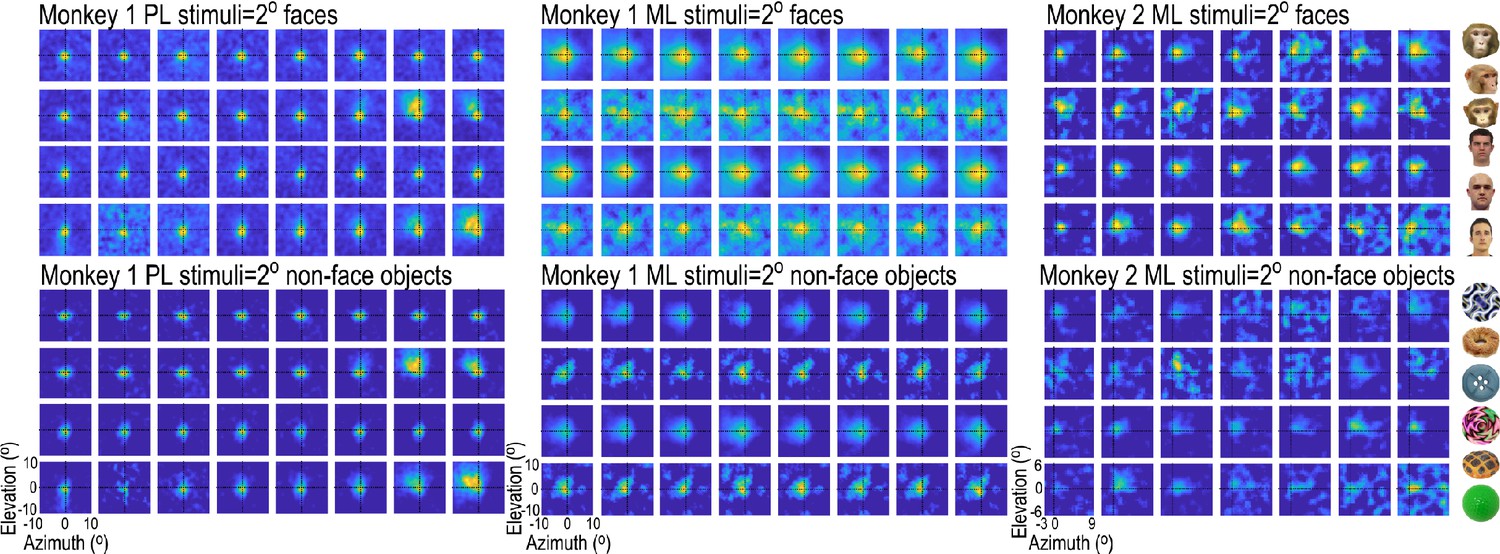
Receptive-field maps for all visually responsive sites in the two arrays in Monkey 1 (both in the right hemisphere) and the single array in Monkey 2 (left hemisphere).
For each site, ~2°x2° images of faces and non-face objects were presented randomly interdigitated in the same recording session, and responses at each site were sorted by image type and normalized to the maximum response at that site. To estimate the response area of receptive fields, a 2D gaussian was fit to each channel’s response map. For RFs mapped with faces, mean (sigma) RF 1.91° +/- 0.27 STD for Monkey 1 PL; 2.30° +/- 0.32 STD for Monkey 1 ML and 2.61° +/- 0.56 STD for Monkey 2 ML. For RFs mapped with non-face objects, mean RF 1.96° +/- 0.23 STD for Monkey 1 PL; 2.23° +/- 0.43 STD for Monkey 1 ML and 2.36 ° +/- 0.49 STD for Monkey 2 ML. Examples of six faces and six non-face objects used for mapping are shown to the right.
Figure 1—figure supplement 3
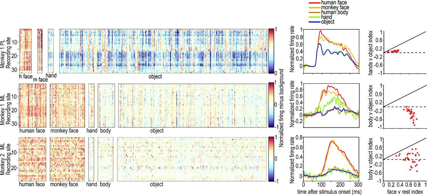
Category selectivity of all visually responsive sites in PL in one monkey (top) and ML in two monkeys (middle and bottom).
The rows in each panel correspond to individual visually responsive recording sites in each electrode array, and the columns correspond to individual images, sorted by category. Images were 4° x 4°. Graphs on the right show PSTHs for each category averaged over all visually responsive sites in each of the electrode arrays in the two monkeys. Category selectivity was measured in Monkey 1 PL and ML in separate recording sessions, and the session for PL did not include bodies. The face selectivity index (face-response – nonface-response)/ (face-response + nonface-response) was greater than 0.3 in all sites in ML in both monkeys, corresponding to a face response at least twice as large as non-face responses (3). The average face selectivity index in Monkey 1 ML was 0.63 (std = 0.06) and in Monkey 2 ML was 0.64 (std = 0.14). The average face vs body selectivity index in Monkey 1 ML was 0.77 (std = 0.11), and in Monkey 2 ML was 0.60 (std = 0.21). The average body vs object selectivity index in Monkey 1 ML was −0.54 (std = 0.17) and in Monkey 2 ML 0.04 (std = 0.27). Face patch PL was less face selective, with an average face selectivity index of 0.24 (std = 0.07) and average hand selectivity index of 0.04 (std = 0.02) Face-selectivity indices were higher than hand or body indices for all channels in both PL and ML. There were no negative mean face or non-face object responses in ML of either monkey but one channel in each of the ML arrays had a below-baseline mean response to bodies, so those channels were not used in calculating the average body vs object indices.
Figure 1—figure supplement 4
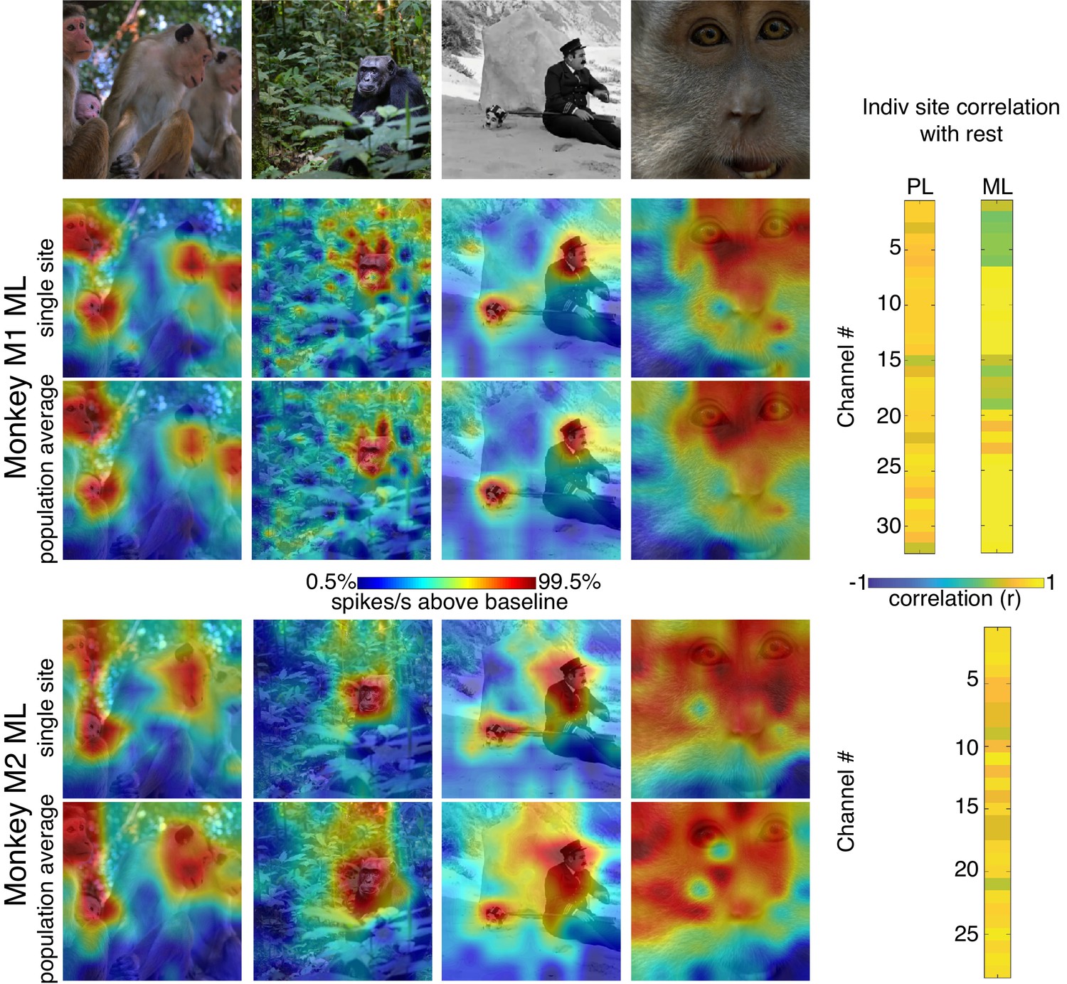
Comparison of single-site response patterns with population average response patterns for all 3 arrays.
(Top row) Images used for correlation mapping. Top left image, still from clip, author ‘Videvo’ (2017) licensed under the ‘Videvo Attribution License’. Any reproduction requires crediting the author. Second image, copyright free photo (CC0) acquired from pxhere.com (2017). Third image, still from The Adventurer, (1917) in the public domain as per publicdomainmovie.net. Fourth image, still from clip, author ‘Videvo’ (2017) licensed under the ‘Videvo Attribution License.’ Any reproduction requires crediting the authors. Firing rates were averaged over 100–250 ms post stimulus onset for Monkey 1 and 150–300 ms for Monkey 2. Responses were scaled to 0.5% and 99.5% percentiles of the response values for each map. (right) Across images, the spatial patterns of responses for individual sites were correlated with average response maps for all other sites for Monkey 1 PL (mean r = 0.73; 0.10 std), Monkey 1 ML (mean r = 0.73; 0.26 std), and Monkey 2 ML (mean r = 0.73; 0.13 std).
Figure 1—figure supplement 5

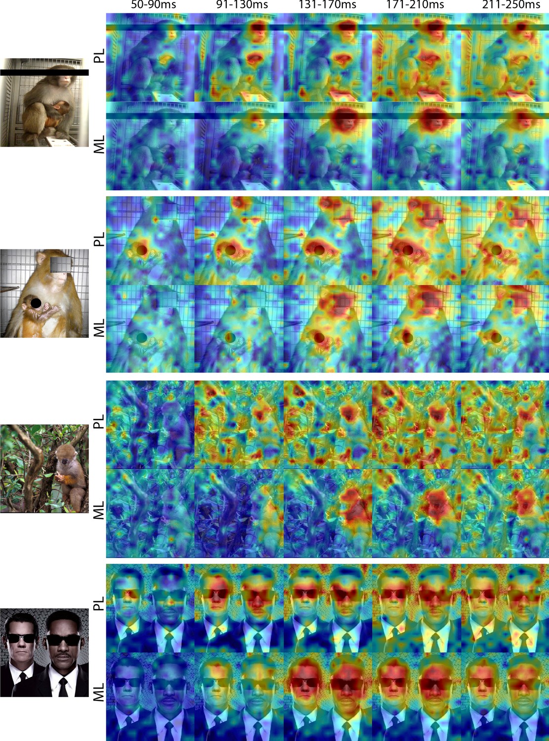
Comparison of response patterns between simultaneously recorded PL and ML arrays in Monkey 1 for different time windows.
Population-level response maps for 40 ms bins between 50 and 250 ms post-stimulus onset. For each image, face-specific activity emerged in PL earlier compared to ML Responses were scaled to 0.5% and 99.5% percentiles of the values for each map.
Figure 2 with 1 supplement

Cells in PL and ML responded to faces with and without eyes.
Population-level response maps from Monkey 1 PL and ML for 40 ms bins between 50 and 250 ms post stimulus onset. Face-specific activity arises in PL prior to ML for images both with and without eyes, even though the latency for each depends on the presence of eyes. (top) Activity specific to eyes emerges earlier than responses to the rest of the face in both PL and ML. (middle and bottom) For both PL and ML, face activity emerges at longer latencies when the eyes are blacked out. Photo courtesy of Ralph Seigel. Response maps scaled to 0.5% and 99.5% percentiles of the response values to each image.
© 2014 Santasombra. All rights reserved. The top-left image is reproduced with permission from Santasombra. It is not covered by the CC-BY 4.0 license and further reproduction of this panel would need permission from the copyright holder.
Figure 2—figure supplement 1
Comparison of response patterns to images of eyeless faces between PL and ML in Monkey 1.
Population-level response maps for 40 ms bins between 50 and 250 ms post-stimulus onset. For each image, face-specific activity emerges in PL earlier than in ML. For both recording sites, face-specific activity emerges later for eyeless faces compared to the same faces with eyes (see also Figure 1—figure supplement 4). Responses were scaled to 0.5% and 99.5% percentiles of the values for each map.
Figure 3 with 3 supplements
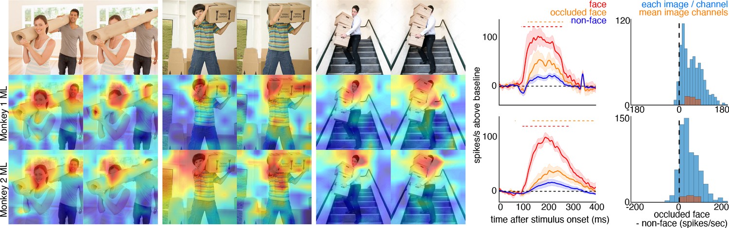
Cells in ML in both monkeys responded to occluded faces.
(top) Images of occluded faces. Population-level response maps from (middle) Monkey 1 ML and (bottom) Monkey 2 ML. Firing rates were averaged over 100–250 ms post stimulus onset for Monkey 1 and 150–300 ms for Monkey 2. Response patterns scaled to 0.5% and 99.5% percentiles of the response values to each image. (right) PSTHs of responses in PL in Monkey 1 to regions of the image with occluded (orange) and non-occluded (red) faces and non-face parts (blue). Shading represents 95% confidence limits. (top) Responses of Monkey 1 ML. (bottom) Responses of Monkey 2 ML. Dashed red (and orange) lines denote time windows with significant differences in response magnitudes between face and occluded-face (and occluded vs. non-face) image parts (paired t-test across 12 images for Monkey 1; t(11) > 2.80 for occluded-face vs. non-face; t(11) > 2.70 for face vs. occluded-face; and 10 images for Monkey 2 t(9) > 2.56 for occluded-face vs. non-face; t(9) > 2.73; p<0.05, FDR-corrected). Note, the small spike just after 300 ms in Monkey 1 is a juicer artifact from the reward delivered after each trial and at least 200 ms prior to the onset of the next stimulus presentation. Histograms show response differences to occluded-face regions minus non-face control regions, for each image, each channel (blue) and for the mean image across channels (orange).
Figure 3—figure supplement 1
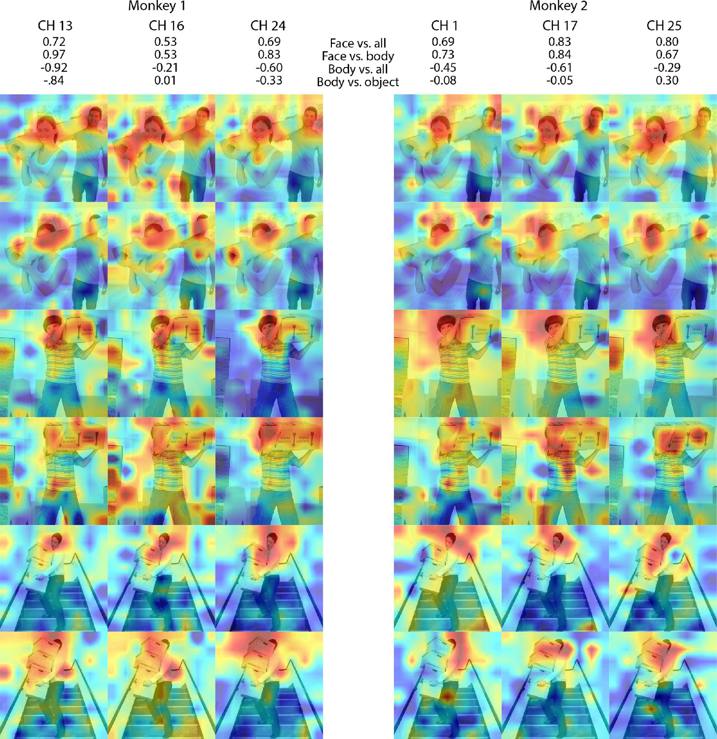
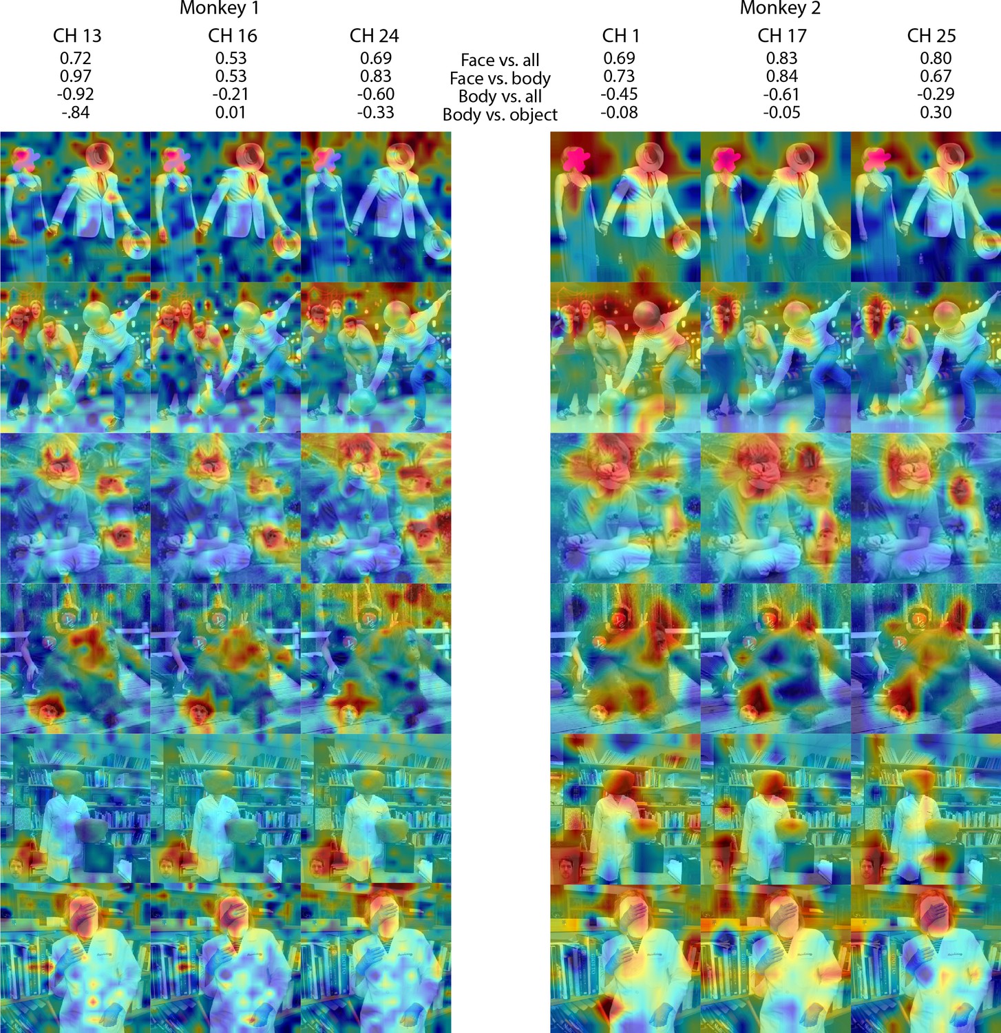
Individual site responses to occluded faces in ML for Monkeys 1 and 2.
Response maps for images reported in Figure 3 from 3 individual channels in (left) Monkey 1 ML and (right) Monkey 2 ML. Face- and body- selectivity indices are shown for each channel. Firing rates were averaged over 100–250 ms post stimulus onset for Monkey 1 and 150–300 ms for Monkey 2. Responses were scaled to 0.5% and 99.5% percentiles of the values for each map. The spatial patterns of responses for individual channels were correlated with average maps for all other sites for Monkey 1 ML intact faces (mean r = 0.87; 0.15 std), Monkey 1 ML occluded faces (mean r = 0.85; 0.14 std), Monkey 2 ML intact faces (mean r = 0.70; 0.14 std), and Monkey 2 ML occluded faces (mean r = 0.47; 0.13 std). Photographs shown in Figure 3.
Figure 3—figure supplement 2

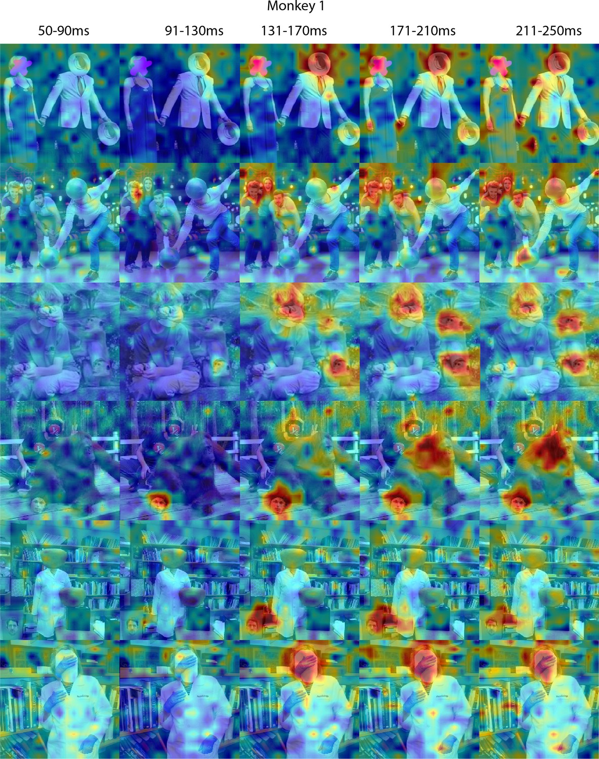
Responses to occluded faces in Monkey 1 ML for different time windows.
Population-level response maps for 40 ms bins between 50 and 250 ms post-stimulus onset. For each image reported in Figure 3, activity where a face ought to be is apparent by 130 ms in ML for monkey 1. Similar to the latency shift observed for masked eyes (Figure 2; Figure 2—figure supplement 1), responses to the occluded faces were delayed relative to non-occluded faces. Responses were scaled to 0.5% and 99.5% percentiles of the values for each map. Photographs shown in Figure 3.
Figure 3—figure supplement 3

Responses to occluded faces in Monkey 2 ML for different time windows.
Population-level response maps for 50 ms bins between 50 and 300 ms post-stimulus onset. For each image reported in Figure 3, activity where a face ought to be is apparent by 150 ms in ML for monkey 2. Similar to the latency shift observed for masked eyes (Figure 2; Figure 2—figure supplement 1), responses to the occluded faces were delayed relative to non-occluded faces. Responses were scaled to 0.5% and 99.5% percentiles of the values for each map. Photographs shown in Figure 3.
Figure 4 with 4 supplements
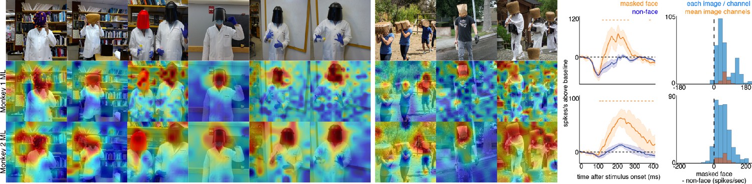
Responses to masked faces.
Cells in ML in both monkeys responded to faces covered by masks, baskets, or paper bags. (top) Images of covered faces. Population-level response maps from (middle) Monkey 1 ML and (bottom) Monkey 2 ML. Firing rates were averaged 100–250 ms post stimulus onset for Monkey 1 and 150–300 ms for Monkey 2. Response patterns scaled to 0.5% and 99.5% percentiles of the response values to each image. (right) PSTHs of responses of sites in ML in Monkeys 1 and 2 to covered faces (orange). Shading represents 95% confidence limits. (top) Responses of sites in Monkey 1 patch ML. (bottom) Responses of sites in Monkey 2 ML. Dashed orange lines denote time windows with significant differences in response magnitudes between covered-face vs. non-face image parts (paired t-test across 10 images for Monkey 1 and 11 images for Monkey 2; t(9) > 2.81 for Monkey 1; t(10) > 2.42 for Monkey 2; p<0.05, FDR-corrected). Histograms show response differences to masked face minus non-face control regions, for each image, each channel (blue) and for the mean image across channels (orange).
Figure 4—figure supplement 1
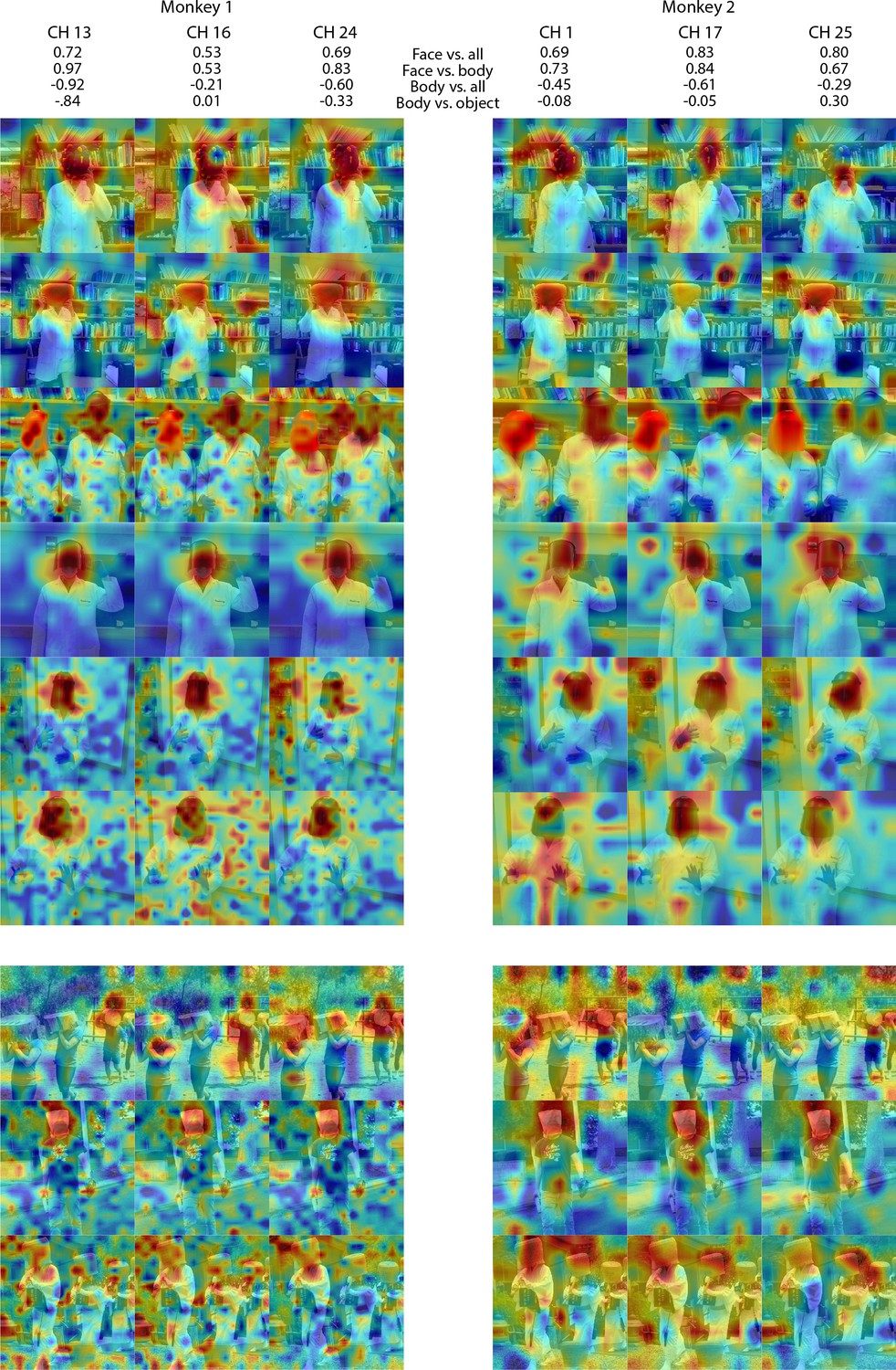
Individual channel responses to masked faces in Monkey 1 and 2 ML.
Response maps for images reported in Figure 4 from 3 individual channels in (left) Monkey 1 ML and (right) Monkey 2 ML. Face- and body- selectivity indices are shown for each channel. Firing rates were averaged over 100–250 ms post stimulus onset for Monkey 1 and 150–300 ms for Monkey 2. Responses were scaled to 0.5% and 99.5% percentiles of the values for each map. The spatial patterns of responses for individual channels were correlated with the average maps for all other sites for Monkey 1 ML (mean r = 0.75; 0.16 std) and Monkey 2 ML (mean r = 0.55; 0.15 std). Photographs shown in Figure 4.
Figure 4—figure supplement 2
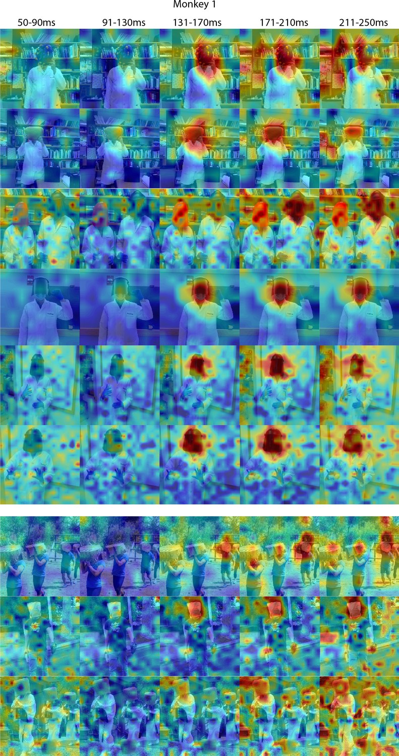
Responses to masked faces in Monkey 1 ML for different time windows.
Population-level response maps for 40 ms bins between 50 and 250 ms post-stimulus onset. For each image reported in Figure 4, activity where a face ought to be is apparent by 130 ms in Monkey 1 ML. Responses were scaled to 0.5% and 99.5% percentiles of the values for each map. Photographs shown in Figure 4.
Figure 4—figure supplement 3
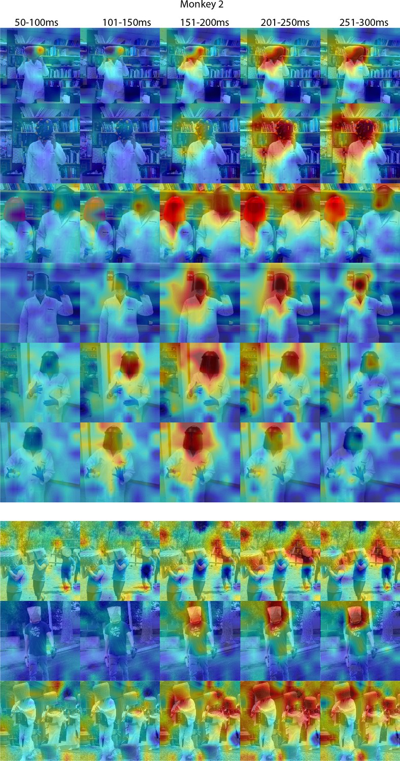
Responses to masked faces in Monkey 2 ML at different time windows.
Population-level response maps for 50 ms bins between 50 and 300 ms post-stimulus onset. For each image reported in Figure 4, activity where the face ought to be is apparent by 150 ms in Monkey 1 ML. Responses were scaled to 0.5% and 99.5% percentiles of the values for each map. Photographs shown in Figure 4.
Figure 4—figure supplement 4

Responses to faces and masked faces in Monkey1 PL.
PSTHs of responses of sites in PL in Monkey 1 to (top) occluded and non-occluded faces, (middle) covered and non-covered faces, and (bottom) non-face images above a body or not above a body. Shading represents 95% confidence limits. Dashed red lines denote time windows with significant differences in response magnitudes between face and occluded face image parts (paired t-test across images; p<0.05, FDR-corrected).
Figure 5 with 3 supplements

Face-like responses to non-face objects.
(top) Manipulated images with non-face objects in positions where a face ought and ought not to be. Population-level response maps from (middle) Monkey 1 ML and (bottom) Monkey 2 ML. Firing rates were averaged 100–250 ms post stimulus onset for Monkey 1 and 150–300 ms for Monkey 2. Response patterns scaled to 0.5% and 99.5% percentiles of the response values to each image. (right) PSTHs of Monkey 1 PL to non-face images above a body (orange) or not above a body (green). (top) PSTHs from Monkey 1 ML. (bottom) PSTHs from Monkey 2 ML. Shading indicates 95% confidence intervals. Dashed orange lines denote time windows with significant differences in response magnitudes between object-atop-body vs. object-apart-from-body (paired t-test across 8 and 15 images for Monkey 1 and 2, respectively; t(7) > 3.04 for Monkey 1; t(14) > 2.38 for Monkey 2; p<0.05, FDR-corrected). Histograms show response differences to object atop body minus object control regions for each image, each channel (blue) and for the mean image across channels (orange).
Figure 5—figure supplement 1
Individual channel face-like responses to non-face objects in Monkey 1 and 2 ML.
Response maps for images reported in Figure 5 from 3 individual channels in (left) Monkey 1 ML and (right) Monkey 2 ML. Face- and body- selectivity indices are shown for each channel. Firing rates were averaged over 100–250 ms post stimulus onset for Monkey 1 and 150–300 ms for Monkey 2. Responses were scaled to 0.5% and 99.5% percentiles of the values for each map. The spatial patterns of responses for individual channels were correlated with the average maps for all other sites for Monkey 1 ML (mean r = 0.76; 0.20 std) and Monkey 2 ML (mean r = 0.63; 0.17 std).
Figure 5—figure supplement 2
Face-like responses to non-face objects in Monkey 1 ML for different time windows.
Population-level response maps for 40 ms bins between 50 and 250 ms post-stimulus onset. For each image reported in Figure 5, activity where a face ought to be is apparent by 130 ms in Monkey 1 ML. Responses were scaled to 0.5% and 99.5% percentiles of the values for each map. Photographs shown in Figure 5.
Figure 5—figure supplement 3

Face-like responses to non-face objects in Monkey 1 ML for different time windows.
Population-level response maps for 50 ms bins between 50 and 300 ms post-stimulus onset. For each image reported in Figure 5, activity where the face ought to be is apparent by 150 ms in Monkey 2 ML. Responses were scaled to 0.5% and 99.5% percentiles of the values for each map. Photographs shown in Figure 5.
Figure 6 with 3 supplements

Body-below facilitation of face-cell responses to non-face objects but not to faces.
Images of face, noise, face outline, and non-face object (top row) above a body and (second row) without a body. (bottom two rows) PSTHs from ML in Monkeys 1 and 2. Responses were calculated over the same face-shaped region for all images, for 7 different image sets of different individuals. Shading indicates 95% confidence intervals. Dashed colored lines denote time windows with significant differences in response magnitudes between face region above body vs. without body (paired t-test across 7 images; t(6) > 2.79 for noise; t(6) > 3.08 for outlines; t(6) > 2.76 for non-face objects; p<0.05, FDR-corrected). Inset histograms show response differences to the regions atop body minus the corresponding regions of no-body images, for each image, each channel (blue) and for the mean image across channels (orange).
Figure 6—figure supplement 1
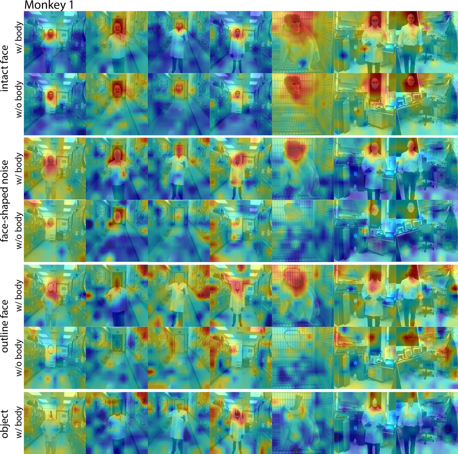
Responses to face and non-face images with and without bodies.
Population-level response maps from Monkey 1 ML for images of intact faces, outlined face, face-shaped noise, and non-face objects above a body and without a body. To illustrate the effect of the body on response maps, each intact face, noise, and outlined image without a body was scaled to the maximum and minimum values of the corresponding image with a body. Object-above- body images were scaled to the min and max responses of the corresponding noise with body. Firing rates were averaged over 100–250 ms. Photographs shown in the section E of Figure 7—figure supplement 3.
Figure 6—figure supplement 2
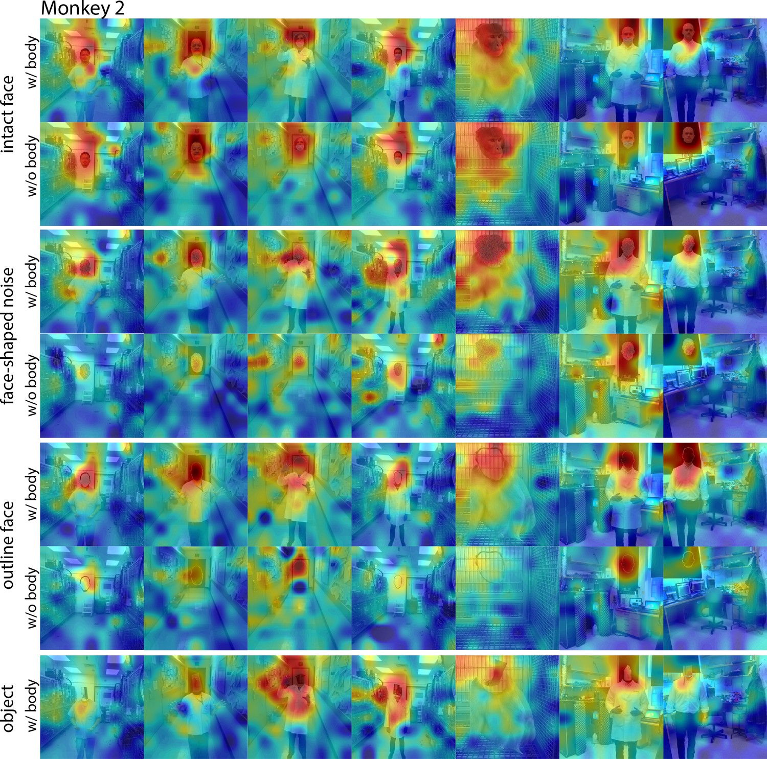
Responses to face and non-face images with and without bodies.
Population-level response maps from Monkey 2 ML for images of intact faces, outlined face, face-shaped noise, and non-face objects above a body and without a body. To illustrate the effect of the body on response maps, each intact face, noise, and outlined image without a body was scaled to the maximum and minimum values of the corresponding image with a body. Object-above-body images were scaled to the min and max responses of the corresponding noise with body. Firing rates were averaged over 150–300 ms post stimulus onset. Photographs shown in section E of Figure 7—figure supplement 3.
Figure 6—figure supplement 3

Responses to the region above bodies in the absence of faces or heads.
(top) Population-level response maps in Monkey 1 ML and Monkey 2 ML to images of faceless mannequins with and without heads. Population-level response maps in Monkey 1 ML and Monkey 2 ML to images of headless bodies with either uniform white or black backgrounds. Firing rates were averaged over 100–250 ms post stimulus onset for Monkey 1 and 150–300 ms for Monkey 2. Responses were scaled to 0.5% and 99.5% percentiles of the values for each map.
Figure 7 with 3 supplements
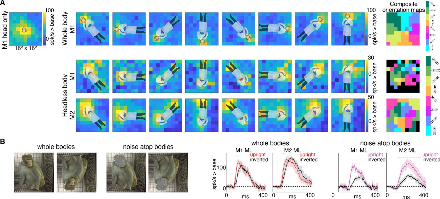
Body-orientation selectivity.
(A) Upper left panel shows an example head-only image overlaid on the population-level activation map averaged across all head only images (n = 8) from Monkey 1 ML. The upper row shows an example whole body image at eight different orientations each overlaid on the average activation maps for all whole bodies (n = 8); maximum responsiveness was focal to the face at each orientation. The lower two rows show a similar spatial selectivity for the region where a face ought to be at each orientation for headless bodies (n = 8) in Monkey 1 and 2 ML. Whole and headless body image sets were presented on a uniform white background (Figure 7—figure supplement 1). The composite maps on the far right show the best body orientation at each grid point for whole bodies and headless bodies for face patch ML in both monkeys, as indicated. The scale of the body orientations from top to bottom corresponds to the body orientations shown left to right in the response maps. Black sections denote areas with responses at or below baseline. For both whole and headless bodies, maximal activation occurred for bodies positioned such that the face (or where the face ought to be) would be centered on the cells’ activating region. (B) PSTHs when whole body and face-shaped noise atop bodies were presented within the cell’s activating region in both monkeys. For whole body images, there was only a brief difference in activity between upright and inverted configurations during the initial response. For face-shaped noise, the response was substantially larger for the upright (vs. inverted) configurations for the duration of the response. Dashed colored lines denote time windows with significant differences in response magnitudes between upright vs. inverted face regions of the image (t-test across 7 images; t(6) > 4.74 for intact faces; t(6) > 3.34 for noise; p<0.05, FDR-corrected).
Figure 7—figure supplement 1
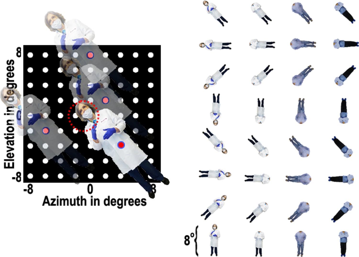
Body-orientation experiment.
Images of 8 different bodies, with or without heads, were presented at various positions in a 9 × 9 grid pattern while the animal fixated on a central fixation spot. Responses were calculated over a 100 ms to 250 ms window after each stimulus presentation.
Figure 7—figure supplement 2
Responses to upright and inverted face and noise images.
Population-level response maps from(top) Monkey 1 ML and (bottom) Monkey 2 ML for upright and inverted images of intact faces with bodies and face-shaped noise with a body. To illustrate the effect of the inversion on response maps, inverted images were scaled to the maximum and minimum values of the corresponding upright versions. Firing rates were averaged over 100–250 ms post stimulus onset for Monkey 1 and 150–300 ms for Monkey 2. Upright and inverted intact face and noise photographs shown in the first and fourth columns in section E of Figure 7—figure supplement 3.
Figure 7—figure supplement 3
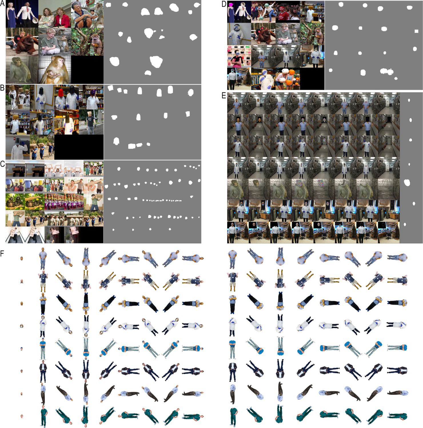
Stimuli used in each experiment and the corresponding binary ROIs of the image regions used for calculating responses or psths corresponding to faces or regions above the body.
(A) Stimuli and ROIs reported in Figure 1. (B) Stimuli and ROIs reported in Figure 4, Figure 4—figure supplements 1–3. (C) Stimuli and ROIs reported in Figure 3, Figure 3—figure supplements 1–3. (D) Stimuli and ROIs reported in Figure 5, Figure 5—figure supplements 1–3. (E) Stimuli and ROIs reported in Figures 6 and 7B, Figure 6—figure supplements 1 and 2, Figure 7—figure supplement 2. (F) Stimuli reported in Figure 7A.
Figure 8 with 1 supplement
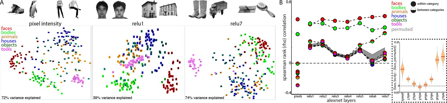
Learned face and body representations in hierarchical artificial neural network (AlexNet).
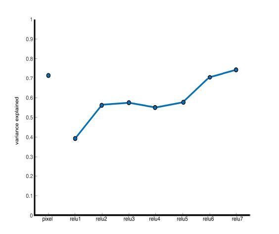
Representational similarity of a stimulus set comprising 240 images across 6 categories including faces and bodies. (A, top) Two example images from each category. (A, bottom) Visualization of similarity between faces (red), bodies (green), houses (blue), objects (green), and tools (pink) from multidimensional scaling of (left column) pixel intensity, (middle column) relu1 units, (right column) relu7 units) Euclidean distances. (B) Comparison of representational similarity within and between categories. Spearman rank correlations were calculated between image pairs based on pixel intensity and activations within AlexNet layers for all object categories. Mean similarity within (solid filled circles) and between (dual colored circles) categories are plotted for pixel intensity and the relu layers of AlexNet. The 2.5% and 97.5% percentiles from a permutation test in which the non-face stimulus labels were shuffled before calculating correlations (grey shaded region) are plotted for pixel and relu layers of AlexNet comparisons. Across all layers, both face and body images are more similar within category than between categories. (inset) The representations of faces and bodies are most similar to each other in deep layers (relu6 and relu7) of AlexNet.
Figure 8—figure supplement 1
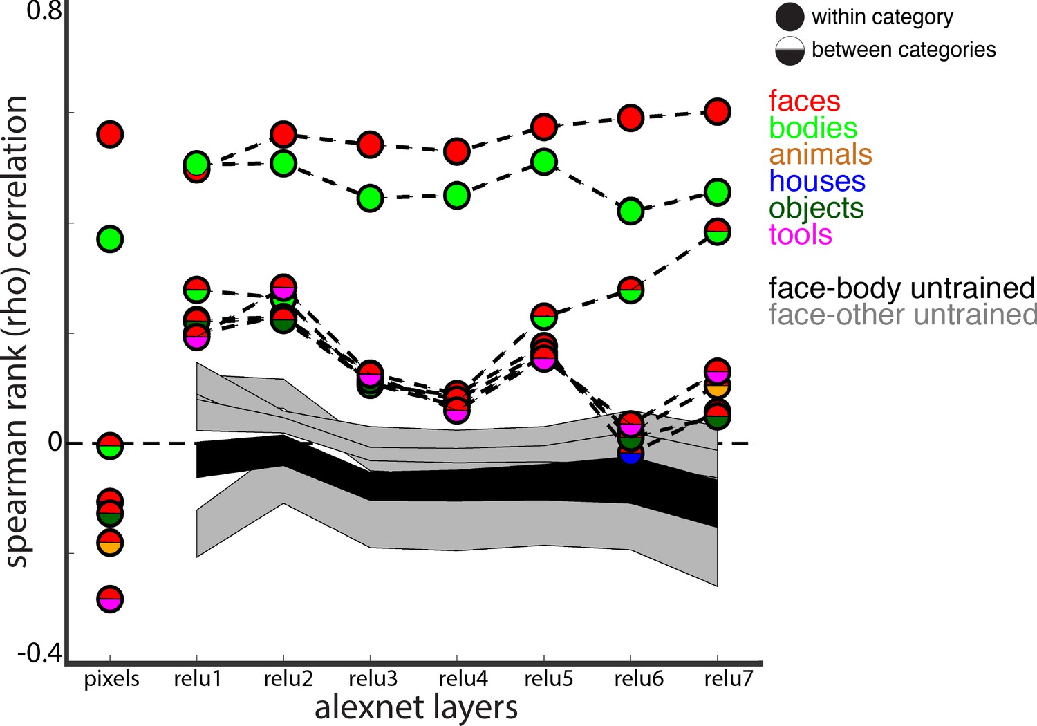
Comparison of correlations between trained and untrained versions of AlexNet.
The 2.5% and 97.5% percentiles from a permutation test in which the weights of the each AlexNet layer were shuffled prior to computing activations are shown for correlations between faces and bodies (black shaded region) and between faces and all other categories (grey shaded regions). Within and between category representational similarity for the pretrained AlexNet reported in Figure 8B are shown for comparison.
Figure 9
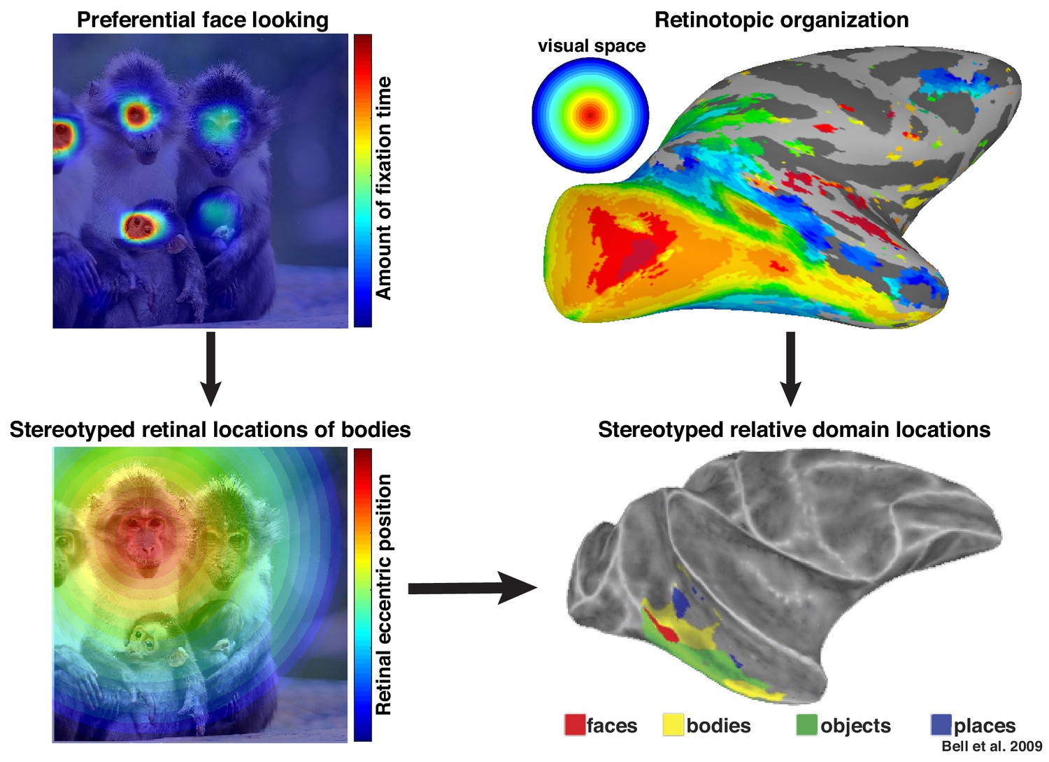
Preferential looking at faces imposes stereotyped retinal experience of bodies.
(top left) Primates spend a disproportionate amount of time looking at faces in natural scenes. (top right) This retinal input is relayed across the visual system in a retinotopic fashion. (bottom left) Example retinal experience of a scene along the eccentricity dimension when fixating a face. Given that bodies are almost always experienced below faces, preferential face looking imposes a retinotopic regularity in the visual experience of bodies. (bottom right) This spatial regularity could explain why face and body domains are localized to adjacent regions of retinotopic IT.
© 2009 American Physiological Society. All rights reserved. Right images reproduced from Bell et al., 2009. They are not covered by the CC-BY 4.0 license and further reproduction of this figure would need permission from the copyright holder.
Author response image 1

Response maps from M1 to natural images without faces.
Hotspots are consistently found over circular shapes and/or above body-life structures.
Author response image 2
Comparison of t-test results with non-parametric Wilcoxon signed-rank test.
Both threshold at p< 0.05 FDR-corrected.
Author response image 3

Author response image 4
Additional files
Download links
A two-part list of links to download the article, or parts of the article, in various formats.
Downloads (link to download the article as PDF)
Open citations (links to open the citations from this article in various online reference manager services)
Cite this article (links to download the citations from this article in formats compatible with various reference manager tools)
The neurons that mistook a hat for a face
eLife 9:e53798.
https://doi.org/10.7554/eLife.53798


