Consistent patterns of distractor effects during decision making
- Department of Rehabilitation Sciences, The Hong Kong Polytechnic University, Hong Kong
- University Research Facility in Behavioral and Systems Neuroscience, The Hong Kong Polytechnic University, Hong Kong
- Wellcome Centre for Integrative Neuroimaging (WIN), Department of Experimental Psychology, University of Oxford, United Kingdom
- FrontLab, Paris Brain Institute (ICM), Inserm U 1127, CNRS UMR 7225, Sorbonne Université, France
Figures
Figure 1 with 2 supplements
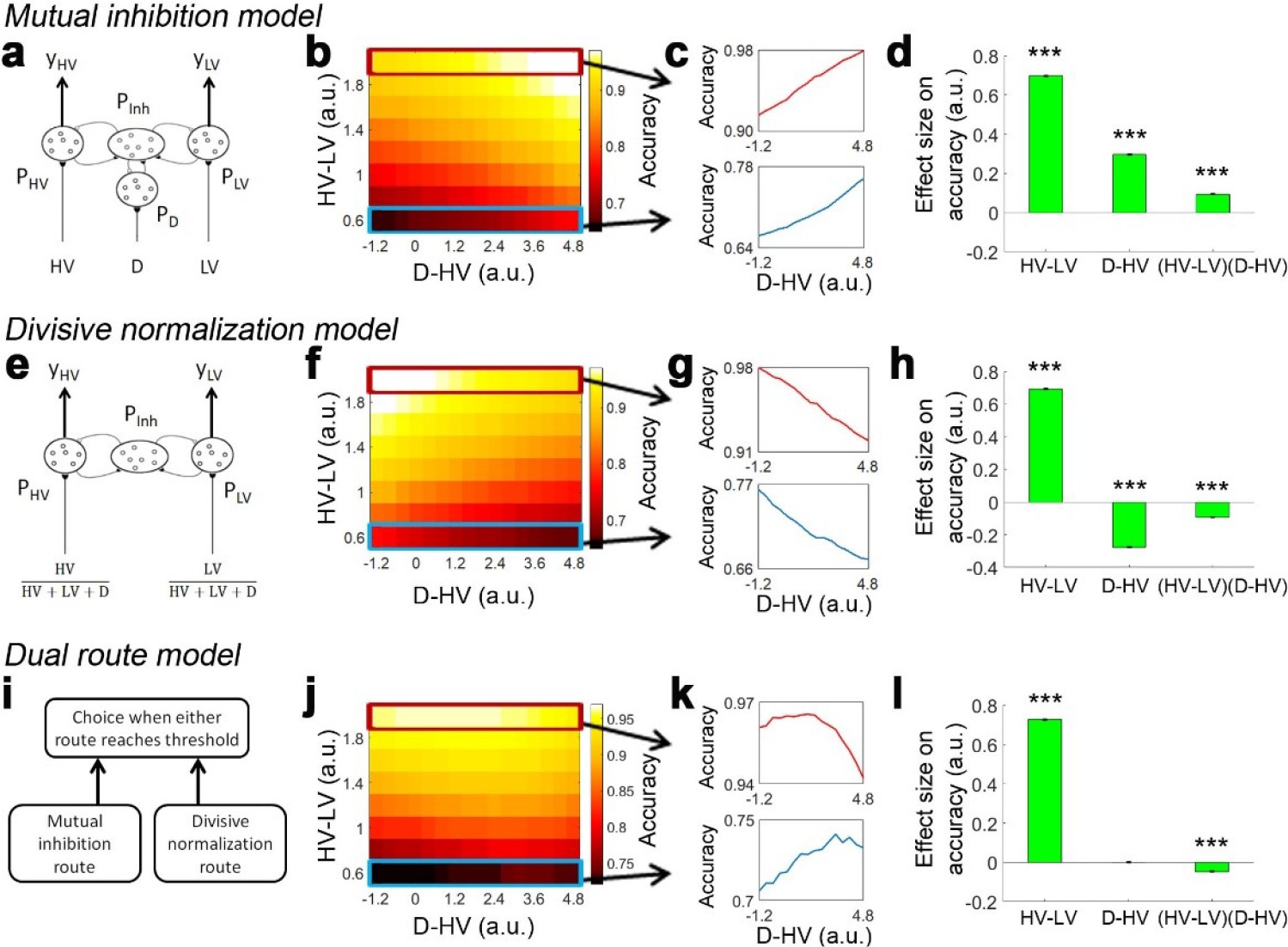
Distractor effects predicted by mutual inhibition model, divisive normalisation model, and a dual route model that combines both other models.
(a) A mutual inhibition model involves three pools of excitatory neurons that receive excitatory input from the HV, LV or D options (PHV, PLV and PD). Concurrently, all excitatory neurons further excite a common pool of inhibitory neurons PInh, which in turn inhibit all excitatory neurons to the same extent. The HV or LV option is chosen once its accumulated evidence (yHV or yLV respectively) reaches a decision threshold. (b) The decision accuracy of the model is plotted across a decision space defined by the difficulty level (i.e. value difference between HV and LV) and the relative distractor value (D–HV). The model predicts a positive distractor effect – the decision accuracy increases (brighter colors) as a function of relative distractor value (left-to-right side). (c) A positive distractor effect is found on both hard (bottom) and easy (top) trials. (d) A GLM analysis shows that the model exhibits a positive HV-LV effect, a positive D-HV effect and a positive (HV-LV)(D–HV) effect. (e) Alternatively, a divisive normalisation model involves only two pools of excitatory neurons that receive input from either the HV or LV option. The input of each option is normalised by the value sum of all options (i.e. HV+LV+D), such that the distractor influences the model’s evidence accumulation at the input level. (f) Unlike the mutual inhibition model, the divisive normalisation model predicts that larger distractor values (left-to-right side) will have a negative effect (darker colours) on decision accuracy. (g) A negative distractor effect is found on both hard (bottom) and easy (top) trials. (h) A GLM analysis shows that the model exhibits a positive HV-LV effect, a negative D-HV effect, and a negative (HV-LV)(D–HV) effect. (i) A dual route model involves evidence accumulation via mutual inhibition and divisive normalisation components independently. A choice is made by the model when one of the components accumulates evidence that reaches the decision threshold. (j) The current model predicts that on hard trials (bottom) larger distractor values (left-to-right side) will have a positive effect (brighter colors) on decision accuracy. In contrast, on easy trials (top) larger distractor values will have a negative effect (the colors change from white to yellow from left to right). (k) The opposite distractor effects are particularly obvious when focusing on the hardest (bottom) and easiest (top) trials. (l) A GLM analysis shows that the model exhibits a positive HV-LV effect, a positive D-HV effect and a negative (HV-LV)(D–HV) effect.
Figure 1—figure supplement 1
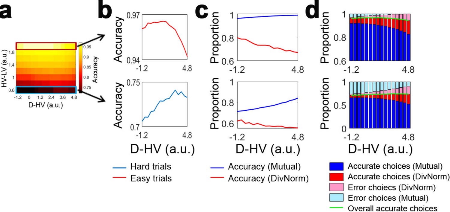
In the dual route model the positive D-HV effect on hard trials is mainly contributed by the mutual inhibition component and the negative D-HV effect on easy trials is mainly contributed by the divisive normalisation component.
(a,b) Replica of Figure 1j and k showing choice accuracy predicted by the dual route model as a function of relative distractor value D-HV and difficulty level. (c) The choices made by the mutual inhibition (Mutual) component and divisive normalisation (DivNorm) components are analysed separately. On hard trials (bottom), accuracy of choices made by the Mutual component (blue lines) increases as a function of D-HV. A similar trend is observed on easy trials (top), but with a smaller slope. In contrast, accuracy of choices made the DivNorm component (red lines) decreases as a function of D-HV in both hard and easy trials and the negative slope is steeper on easy trials. (d) There are overall four possible types of choices made by the dual route model – accurate and error choices made by the Mutual component and accurate and error choices made by the DivNorm component. (Bottom) On hard trials, in choices made by the Mutual component the proportion of errors (light blue bars) decreases much more rapidly than the accurate choices (dark blue bars) as a function of D-HV. In choices made by the DivNorm component, the proportions of accurate (red) and error (pink) choices made by the divisive normalisation model increase to a similar extent. Thus, there is an overall net increase in accuracy on hard trials as a function of D-HV. (Top) In contrast, on easy trials errors made by the Mutual component are rare and there is little variability as a function of D-HV. However, errors made by the divisive normalisation component increase as a function of D-HV. Thus, there is an overall net decrease in accuracy on easy trials as a function D-HV. The green lines show the proportion of overall accurate choices, which are identical to the lines on panel b.
Figure 1—figure supplement 2
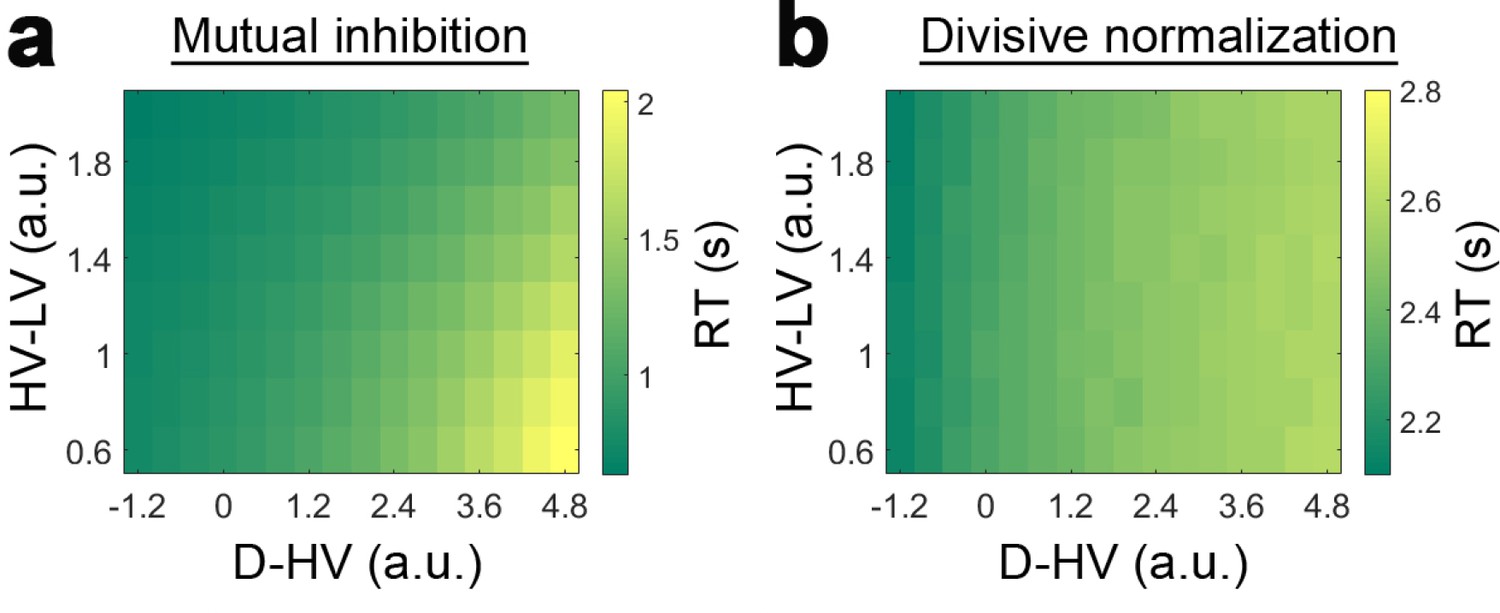
Reaction time (RT) of choices made by the dual route model.
(a) RT of the mutual inhibition component when the divisive normalisation component is switched off. (b) RT of the divisive normalisation component when the mutual inhibition component is switched off. Although the RT of the mutual inhibition component is generally faster than that of the divisive normalisation component, due to variability in the RTs of both components, choices are sometimes made by the divisive normalisation component (see Figure 1—figure supplement 1d).
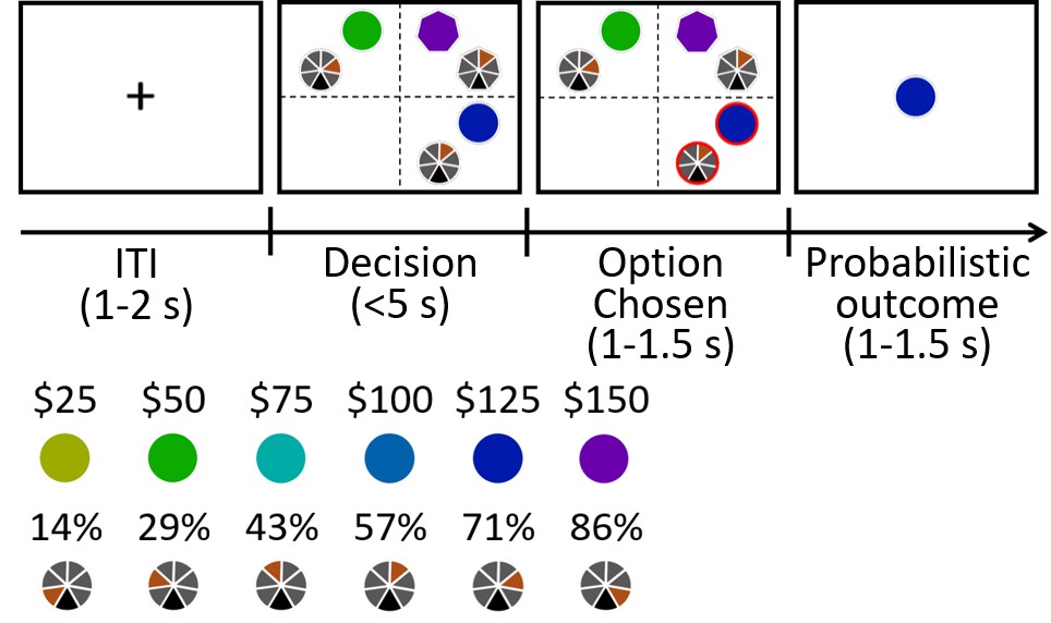
Figure 2
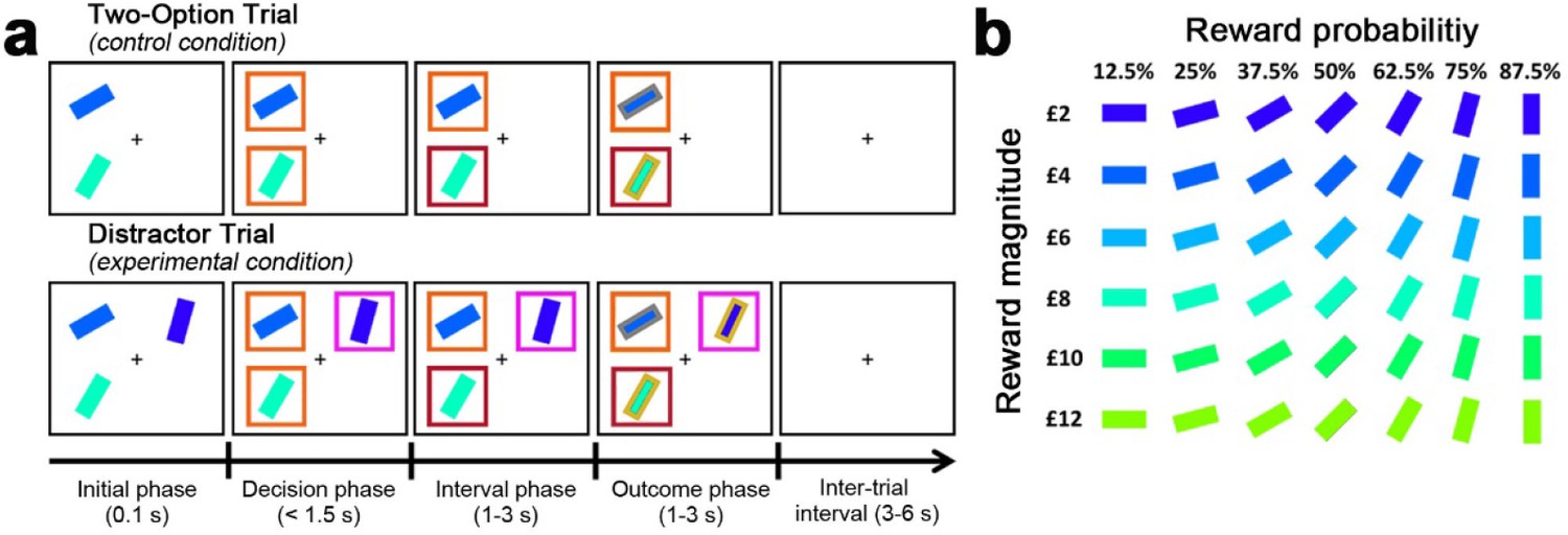
Behavioural task in Experiments 1–7.
(a) The behavioural task was first described by Chau et al., 2014 as follows. In the initial phase of two-option trials participants saw two stimuli indicating two choices. These were immediately surrounded by orange squares, indicating that either might be chosen. A subsequent color change in one box indicated which choice the participant took. In the outcome phase of the trial the outline color of the chosen stimulus indicated whether the reward had been won. The final reward allocated to the participant on leaving the experiment was calculated by averaging the outcome of all trials. Distractor trials unfolded in a similar way but, in the decision phase, one stimulus, the distractor, was surrounded by a purple square to indicate that it could not be chosen while the presentation of orange squares around the other options indicated that they were available to choose. (b) Prior to task performance participants learned that stimulus orientation and color indicated the probability and magnitude of rewards if the stimulus was chosen.
© 2014 Springer Nature. Figure 2 is reproduced from Chau et al., 2014, Nature Neuroscience, by permission of Springer Nature (copyright, 2014). This figure is not covered by the CC-BY 4.0 licence and further reproduction of this panel would need permission from the copyright holder.
Figure 3 with 3 supplements
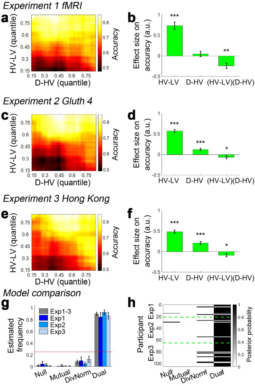
Decision accuracy across the decision space.
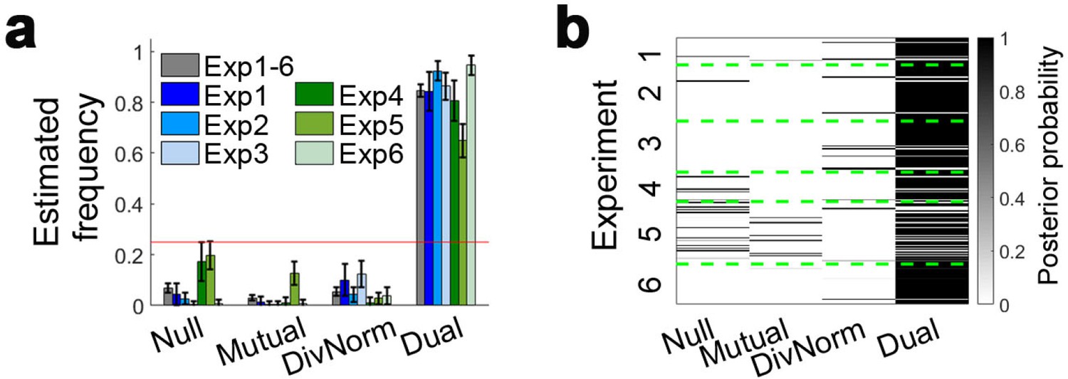
Accuracy (light-yellow indicates high accuracy, dark-red indicates low accuracy) is plotted across the decision space defined by decision difficulty (HV-LV) and relative distractor value (D–HV) from (a) Experiment 1 fMRI2014, (c) Experiment 2 Gluth4, (e) Experiment 3 Hong Kong. In the case of each experiment, GLM analysis indicates that similar factors influence accuracy. The difference in value between the better and worse choosable option (HV-LV) is a major influence on accurately choosing the better option HV. However, accurate choice of HV is also more likely when the distractor is high in value (D-HV is high) and this effect is more apparent when the decision is difficult (negative interaction of (HV-LV)(D–HV)) in the data from (b) Experiment 1 fMRI2014, (d) Experiment 2 Gluth4, (f) Experiment 3 Hong Kong. (g) A model comparison shows that participants’ behaviour in Experiments 1 to 3 is best described by the dual route model, as opposed to the null, mutual inhibition, or divisive normalisation models. (h) Posterior probability of each model in accounting for the behaviour of individual participants. Null: null model; Mutual: mutual inhibition model; DivNorm: divisive normalisation model; Dual: dual route model. *p<0.05, **p<0.01, ***p<0.001. (a–f) Error bars indicate standard error. (g–h) Error bars indicate standard deviation.
Figure 3—figure supplement 1
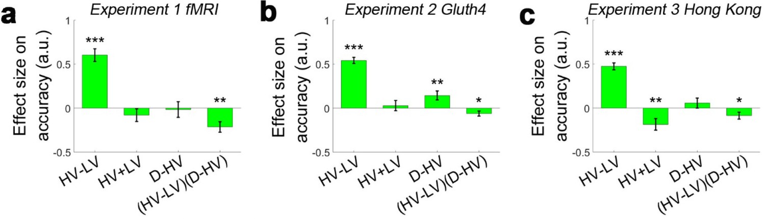
A similar (HV-LV)(D–HV) effect was observed when the HV+LV term was added to GLM1a which was done in GLM1b.
A negative (HV-LV)(D–HV) interaction effect was found in (a) Experiment 1, (b) Experiment two and (c) Experiment 3. *p<0.05, **p<0.01, ***p<0.001. Error bars indicate standard error.
Figure 3—figure supplement 2
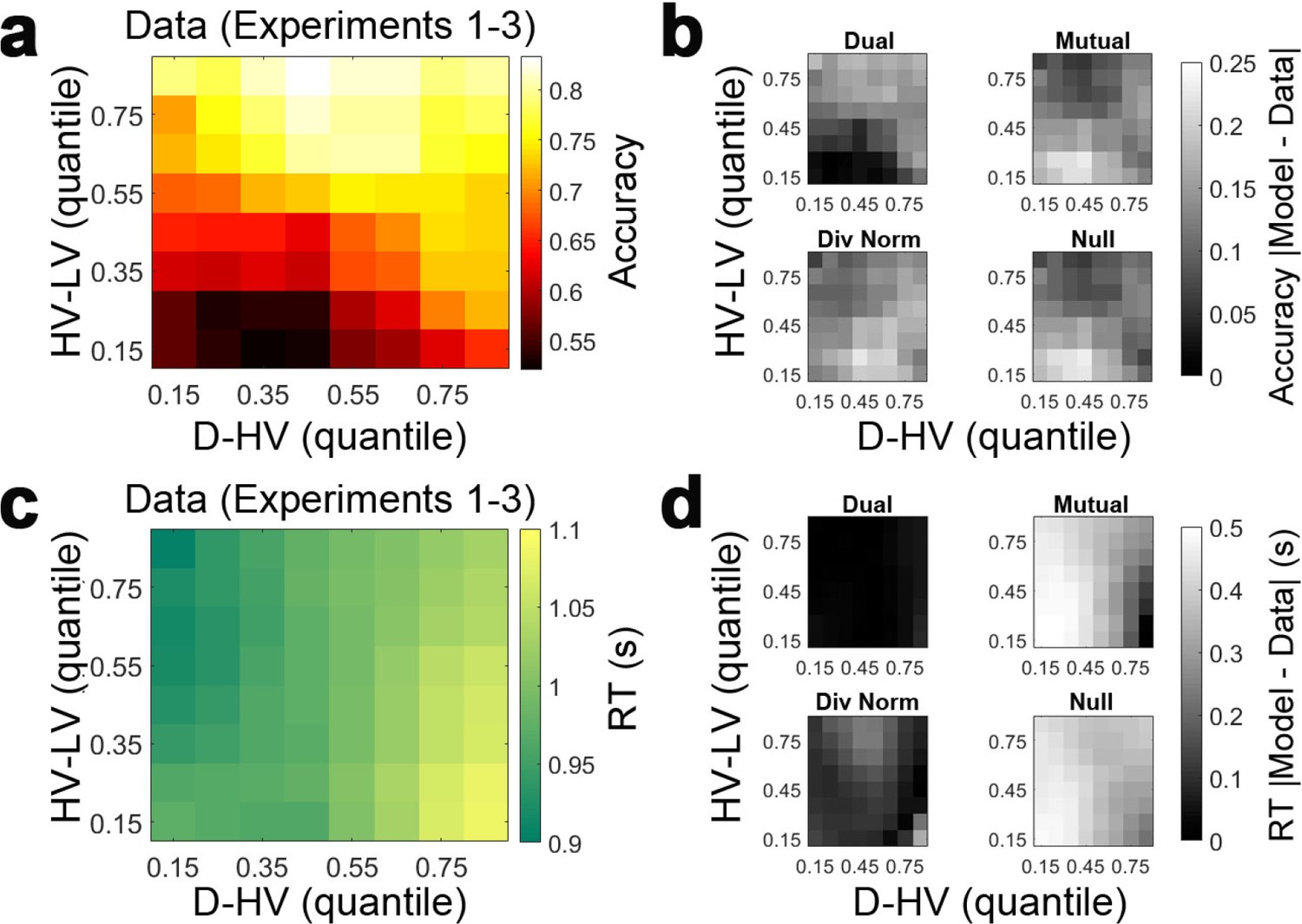
The dual route model is better than the mutual inhibition, divisive normalisation and null models in predicting participants’ accuracy and reaction time.
(a) A plot showing the choice accuracy of participants of Experiments 1–3 as a function of HV-LV and D-HV. In other words, it shows the averaged data of Figure 3a,c,e. (b) The fitted parameters were applied back to the corresponding models to predict choices in the exact same trials that the participants performed. The predictions were repeated for 1000 iterations and the absolute deviation of the predictions from the empirical data was calculated (i.e. absolute difference between models’ and participants’ accuracy). The results show that overall the dual route model (top-left) is better than (darker colors) the mutual inhibition (top-right), divisive normalisation (bottom-left) and null (bottom-right) models in predicting participants’ accuracy. The same procedure was then repeated to test the models’ prediction of reaction time (RT). (c) Participants’ reaction times were slower (yellow colors) on trials that were harder (bottom rows) and with larger distractor values (right columns). (d) As in (b), the absolute deviation in RT between models’ predictions and participants’ behaviour is plotted. The dual route model (top-left) is better than (darker colors) the mutual inhibition (top-right), divisive normalisation (bottom-left) and null (bottom-right) models in predicting participants’ RT.
Figure 3—figure supplement 3
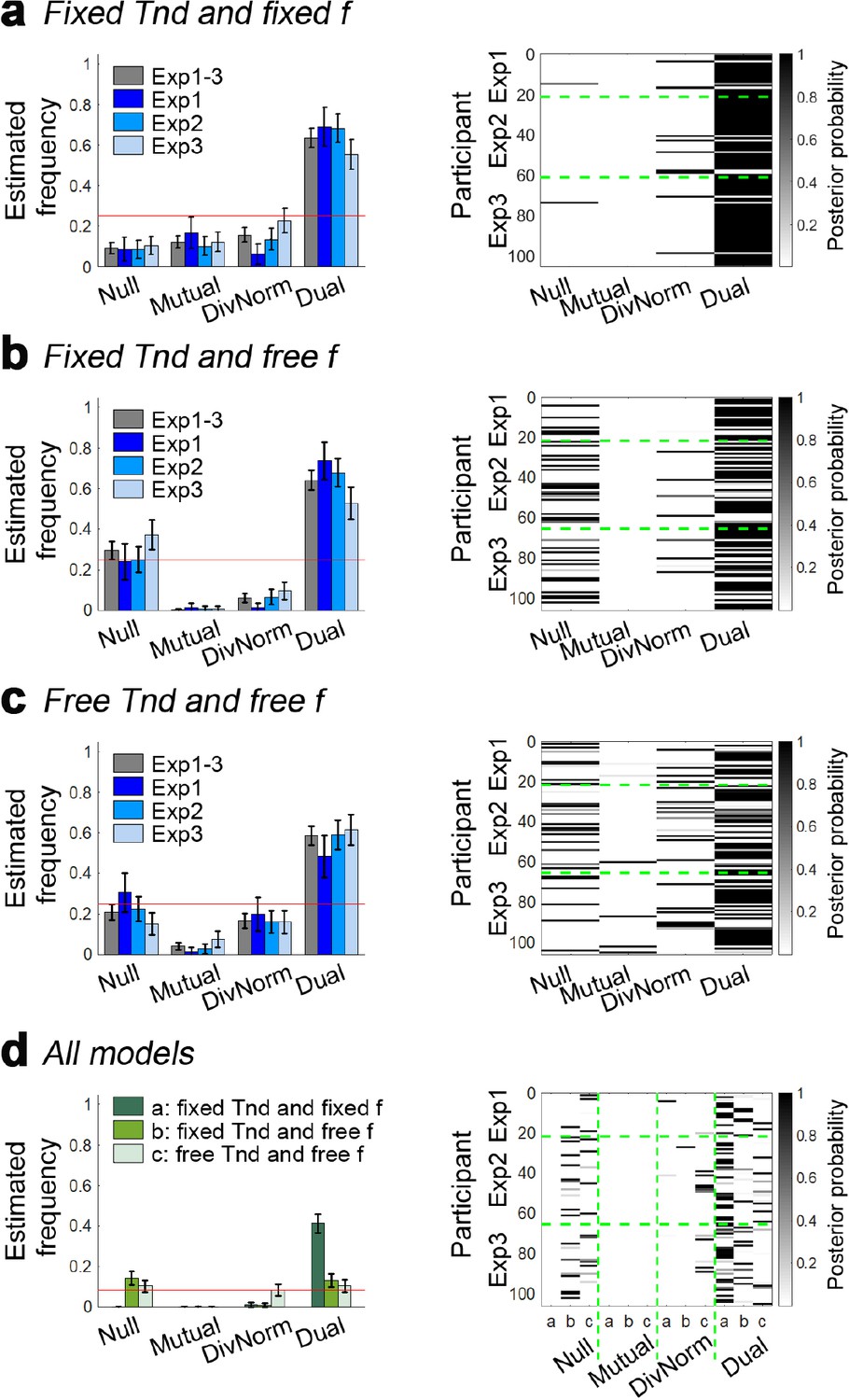
The dual route model provides the best account of participants’ behaviour regardless of the parameterisation of non-decision time Tnd and inhibition level f.
(a) Replica of Figure 3g and h. In this set of models, Tnd is fixed at 0.3 s and f is fixed at 0.5. (b) In this set of models, Tnd is fixed at 0.3 s and f is a free parameter with a prior at 0.5. In the dual route model, the f of each route is fitted independently. (c) In this set of models, Tnd is a free parameter with a prior at 0.3 s and f is also a free parameter with a prior at 0.3. In all three versions of model set, the dual route model provide the best fit of participants’ behaviour. (d) All twelve models in a–c) are compared in a single analysis. The dual route model with fixed Tnd and f provides the best account of participant behaviour (Ef = 0.413, Xp = 1.000). Null: null model; Mutual: mutual inhibition model; DivNorm: divisive normalisation model; Dual: dual route model. Error bars indicate standard deviation.
Figure 4 with 2 supplements

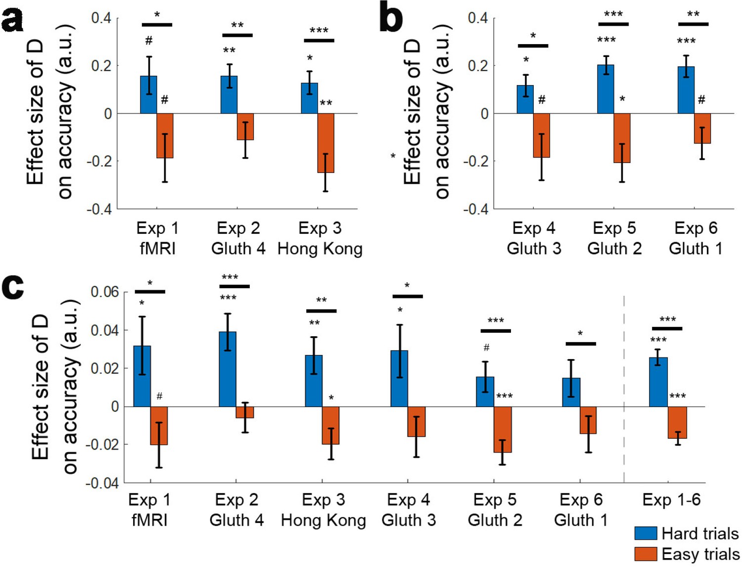
Distractors had opposite effects on decision accuracy as a function of difficulty in all experiments.
The main effect of the distractor was different depending on decision difficulty. (a) In accordance with the predictions of the dual route model, high value distractors (D-HV is high) facilitated decision making when the decision was hard (blue bars), whereas there was a tendency for high value distractors to impair decision making when the decision was easy (red bars). Data are shown for (b) Experiment 1 fMRI2014, Experiment 2 Gluth4, Experiment 3 Hong Kong. (c) The same is true when data from the other experiments, Experiments 4–6 (i.e. Gluth1-3), are examined in a similar way. However, participants made decisions in these experiments in a different manner: they were less likely to integrate probability and magnitude features of the options in the optimal manner when making decisions and instead were more likely to choose on the basis of a weighted sum of the probability and magnitude components of the options. Thus, in Experiments 4–6 (i.e. Gluth1-3), the difficulty of a trial can be better described by the weighted sum of the magnitude and probability components associated with each option rather than the true objective value difference HV-LV. This may be because these experiments included additional ‘decoy’ trials that were particularly difficult and on which it was especially important to consider the individual attributes of the options rather than just their integrated expected value. Whatever the reason for the difference in behaviour, once an appropriate difficulty metric is constructed for these participants, the pattern of results is the same as in panel a. # p<0.1, *p<0.05, **p<0.01, ***p<0.001. Error bars indicate standard error.
Figure 4—figure supplement 1
Similar difficulty-dependent distractor effects were observed when accuracy is explained using the value of D, rather than the relative value of D in comparison to HV (i.e. D–HV).
(a) Positive and negative D effects were found on hard and easy trials respectively in Experiments 1 fMRI2014, Experiment 2 Gluth4, and Experiment 3 Hong Kong, using GLM2b. As in Figure 4a, difficulty was described by HV-LV in these experiments. (b) The same pattern of D effects was also found in Experiments 4–6 (Gluth1-3) when difficulty was described by a weighted sum of the probability and magnitude components of the options, as in Figure 4b (GLM2d). (c) It is also possible to observe similar difficulty-dependent distractor effects in all six experiments by analysing all data with one single approach. First ‘novel’ trials in Experiments 2, 4–6, added by Gluth and colleagues to test decoy effects were excluded. Then choice difficulty was estimated based on a combination of HV-LV and HV+LV, instead of either the HV-LV difference or the weighted sum of magnitude and probability differences. Here HV+LV was also included because it is possible that the total value sum also contributes to the subjective difficulty level. Finally, GLM2b was applied to estimate the effect of D on hard and easy trials. # p<0.1, *p<0.05, **p<0.01, ***p<0.001. Error bars indicate standard error.
Figure 4—figure supplement 2
The dual-route model best describes participant behaviour in Experiments 1–6.
(a) A model comparison shows that participant behaviour in Experiments 4 to 6, as well as Experiments 1–3 (Figure 3g–h), is best described by the dual route model, as opposed to the null, mutual inhibition, or divisive normalisation models. (b) Posterior probability of each model in accounting for the behaviour of individual participants. Null: null model; Mutual: mutual inhibition model; DivNorm: divisive normalisation model; Dual: dual route model. Error bars indicate standard deviation.
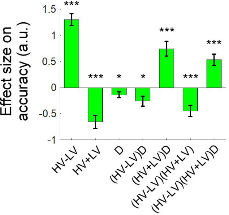
Figure 5
A further replication of distractor effects in 174 participants.
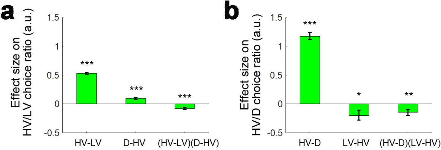
On some occasions ‘attentional capture’ occurs and participants, contrary to their instructions choose the distractor itself. It is possible to analyse how participants distribute their choices between the choosable options HV and LV and between the high value choosable option HV and the distractor D using multinomial logistic regression. (a) Multinomial regression confirms that HV is chosen over LV if the HV-LV difference is large but also confirms that there is an interaction between this term and the difference in value between D and HV. (b) There are also, however, parallel effects when decisions between HV and D are now considered. In parallel to the main effect seen in decisions between HV and LV, decisions between HV and D are mainly driven by the difference in value between these two chooseable options – the HV-D difference. In parallel to the distractor effect seen when decisions are made between HV and LV, there is also an effect of the third option, now LV, when decisions between HV and D are considered; there is an (HV-D)(LV-HV) interaction. *p<0.05, **p<0.01, ***p<0.001. Error bars indicate standard error.
Figure 6
Loss Experiment.
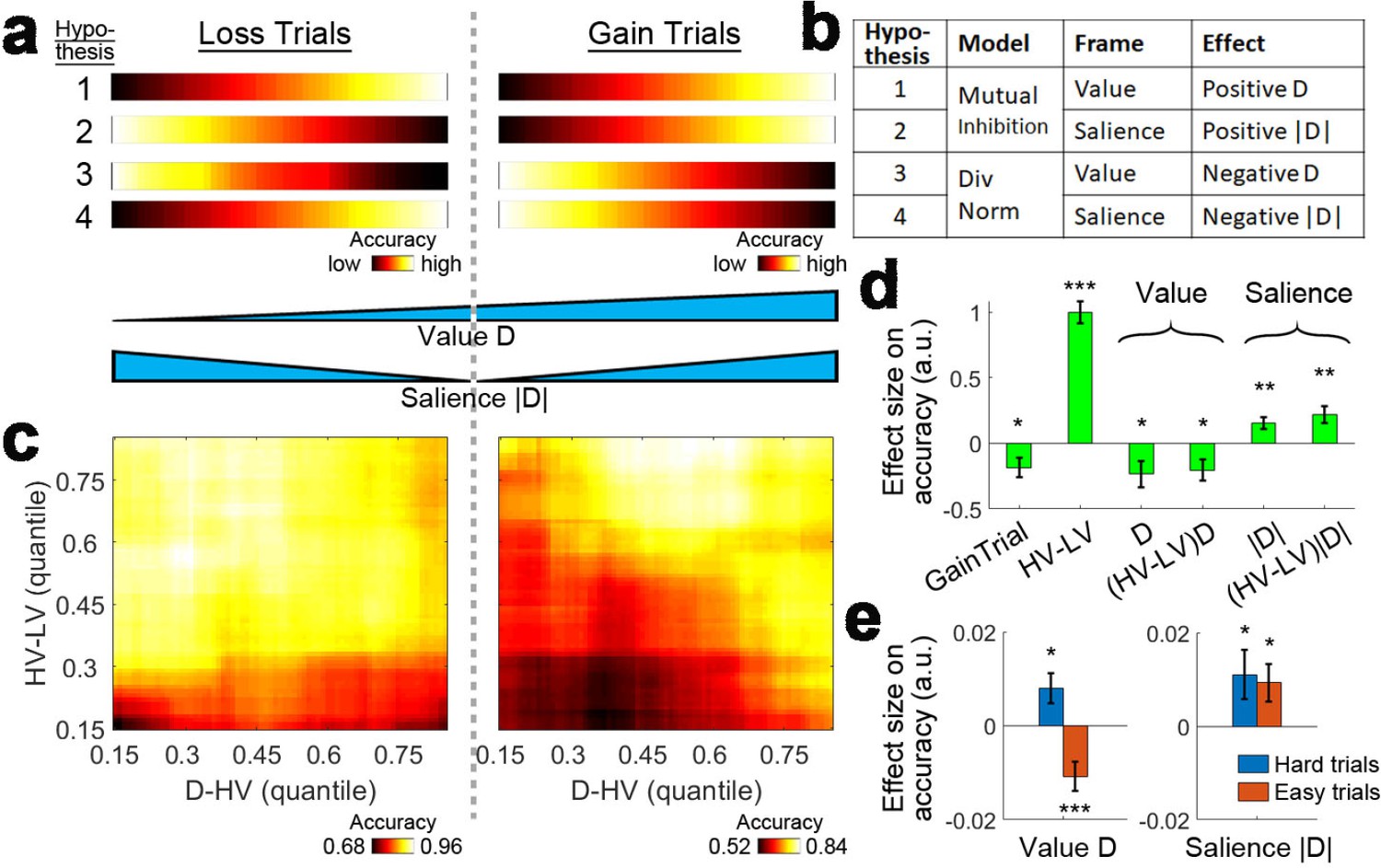
(a, bottom) Value and salience are collinear when values are only related to rewards (right half) but it is possible to determine whether each factor has an independent effect by also looking at choices made to avoid losses (both left and right halves). (a, top and b) Four hypothetical effects of distractor on accuracy. The first and second hypotheses suggest that the distractor effect is positive, which is predicted by the mutual inhibition model and is related to the distractor’s value and salience respectively. The third and fourth hypotheses suggest that the distractor effect is negative, which is predicted by the divisive normalisation model, and is related to its value and salience respectively. All four hypothesis are not mutually exclusive – value and salience are orthogonal factors and positive/negative distractor effects can predominate different parts of decision space. (c, right) A plot identical to that in Figure 3e that shows the data from the gain trials of Experiment 3 Hong Kong. Accuracy (light-yellow indicates high accuracy, dark-red indicates low accuracy) is plotted across the decision space defined by decision difficulty (HV-LV) and relative distractor value (D–HV). (c, left) A similar plot using the data from the loss trials of Experiment 7 Loss Experiment is shown. (d) GLM analysis indicates the distractor value D had a negative effect, suggesting that accuracy was more impaired on trials with distractors that were associated with fewer losses or more gains. In contrast, the distractor salience |D| had a positive effect, suggesting that accuracy was more facilitated on trials with more salient distractors (i.e. those related to larger gains or losses). (e, left) The negative value D effect was significant on easy trials (orange) and reversed and became positive on hard trials (blue). (e, right) In contrast, the positive salience |D| effect was significant on both hard and easy trials. In the dual route model, there are two components that guide decision making in parallel. This pattern suggests that the positive distractor effect of the mutual inhibition component is related to the salience and value of the distractor whereas the negative distractor effect of the divisive normalisation component is most closely related to the value of the distractor. *p<0.05, **p<0.01, ***p<0.001. Error bars indicate standard error.
Figure 7 with 1 supplement
Experiment 8: eye tracking experiment.
The behavioural paradigm was adapted from that used in Experiments 1–7. (a) Each choosable option was represented by a pair of circles. Each distractor option was represented by a pair of heptagons. The screen was divided into four quadrants and each quadrant had two positions for presenting a pair of stimuli associated with an option, making up a total of eight positions. The eight positions were all 291 pixels from the center of the screen and equally separated. Options and distractors appeared in different quadrants on each trial. (b) The reward magnitude of an option/distractor was represented by the color of one component stimulus whereas the angle of the tick on the other component stimulus indicated reward probability.
Figure 7—figure supplement 1
As in Experiments 1–6, in Experiment eight the distractor effect was modulated as a function of difficulty and the total value of the choosable options.
The choice accuracy data in Experiment eight was analysed by GLM5 that includes all main effects of HV-LV, HV+LV, and D and also the two- and three-way interactions involving these terms. Similar to Experiments 1–6, the (HV-LV)D interaction is negative and the (HV+LV)D interaction is positive. These suggest that the distractor effect on decision accuracy was particularly positive when decisions were difficult and also when the total HV+LV value was large. *p<0.05, **p<0.01, ***p<0.001. Error bars indicate standard error.
Figure 8 with 1 supplement

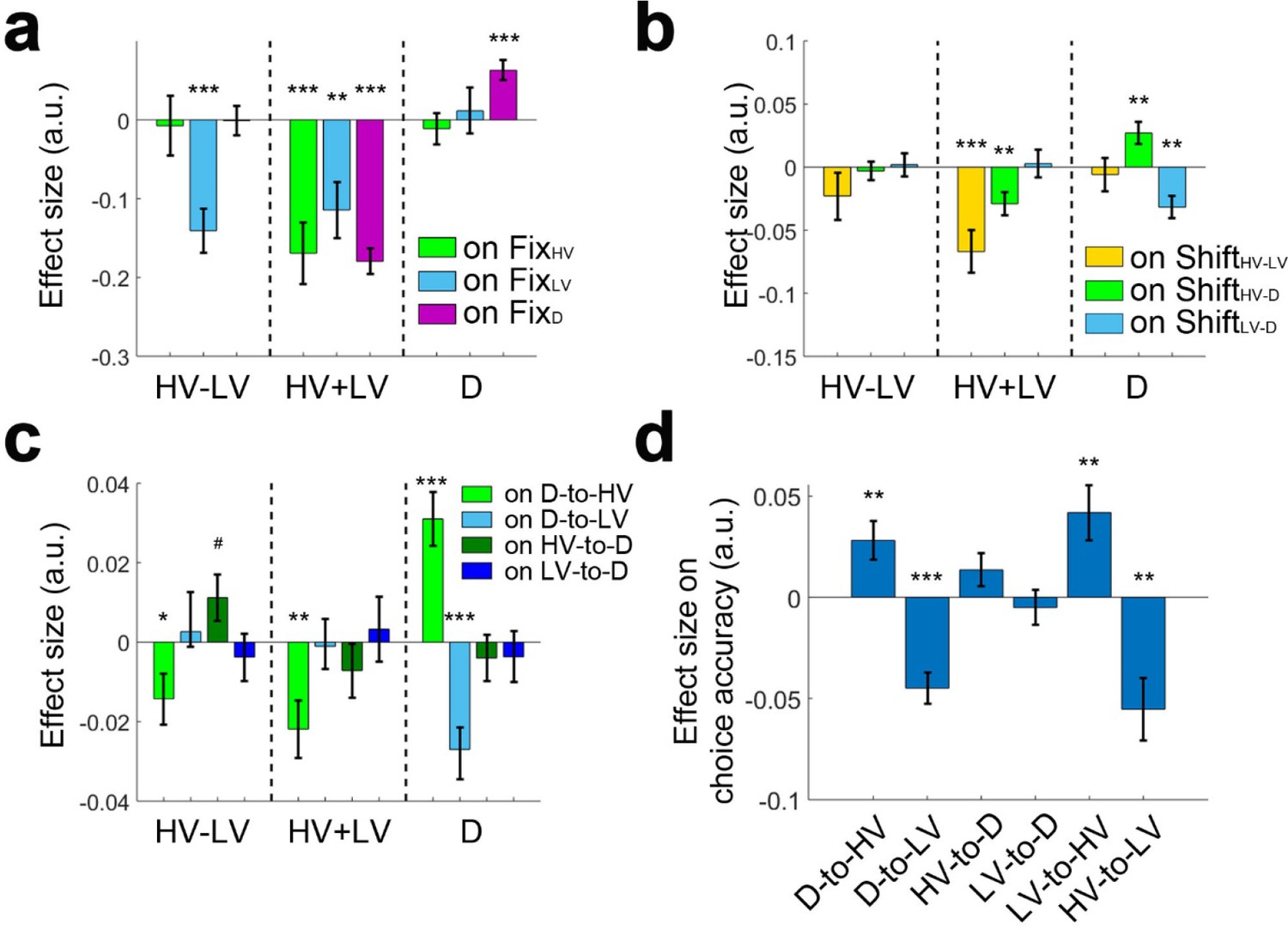
Larger D values were associated with more gaze shifts from D to HV and more accurate decisions.
(a) A multivariate regression analysis showed that larger D values were associated with attentional capture effects as indexed by more fixations at D (right, purple bar). In addition, larger HV-LV difference was associated with fewer fixations at LV (left, blue bar) and larger total HV+LV values were associated with fewer fixations in general (middle). (b) As D value increased so did gaze shifts between D and HV (right, green bar), while gaze shifts between D and LV decreased (right, blue bar). These effects could not merely be due to more fixations at HV or LV per se because the effects of fixations at HV, LV and D on the gaze shifts were partialled out before testing the relationships between D value and gaze shifts. (c) The effect was directionally specific; larger D values were associated with more D-to-HV shifts and fewer D-to-LV shifts but not the opposite (right, green and blue bars; HV-to-D or LV-to-D shifts). (d) In turn, more D-to-HV shifts and fewer D-to-LV shifts predicted greater decision accuracy. FixHV fixation at HV; FixLV fixation at LV; FixD fixation at D; ShiftHV-LV gaze shift between HV and LV; ShiftHV-D gaze shift between HV and D; ShiftLV-D gaze shift between LV and D. # p<0.1, *p<0.05, **p<0.01, ***p<0.001. Error bars indicate standard error.
Figure 8—figure supplement 1
The same analysis performed in Figure 8 was performed by including one additional participant and the results remained similar.
A posterior power analysis indicated that 22 participants were required to meet a power of 80% and alpha of 0.05. Initially an inclusion criterion of eye movement data validity >85% resulted in 21 participants, which is one participant less than the required number. Then, the inclusion criterion was relaxed to 70% to include one additional participant (i.e. n = 22). The results remained similar to those reported in Figure 8. FixHV fixation at HV; FixLV fixation at LV; FixD fixation at D; ShiftHV-LV gaze shift between HV and LV; ShiftHV-D gaze shift between HV and D; ShiftLV-D gaze shift between LV and D. *p<0.05, **p<0.01, ***p<0.001. Error bars indicate standard error.
Figure 9 with 1 supplement
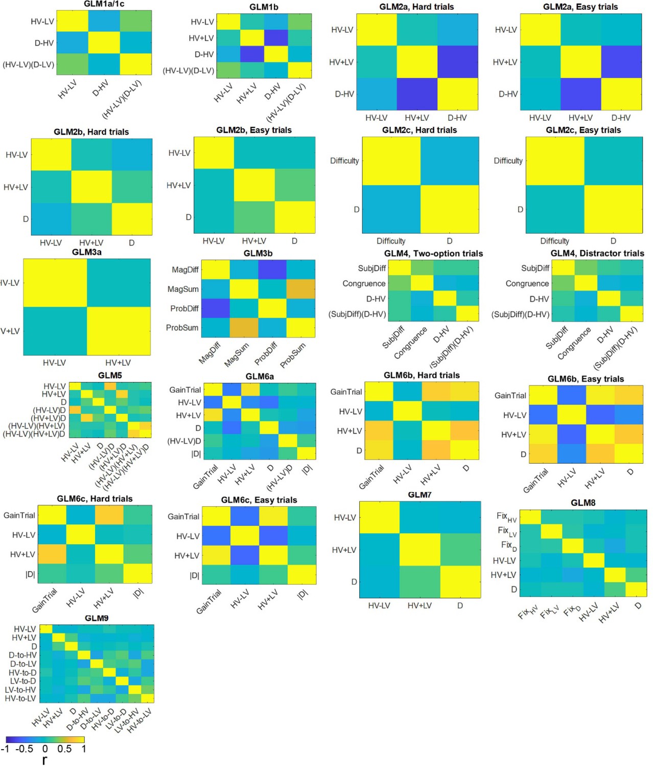
Correlations between regressors.
Each plot shows the levels of correlation between regressors in the general linear models used. Correlation is presented as Pearson’s r averaged across participants.
Figure 9—figure supplement 1
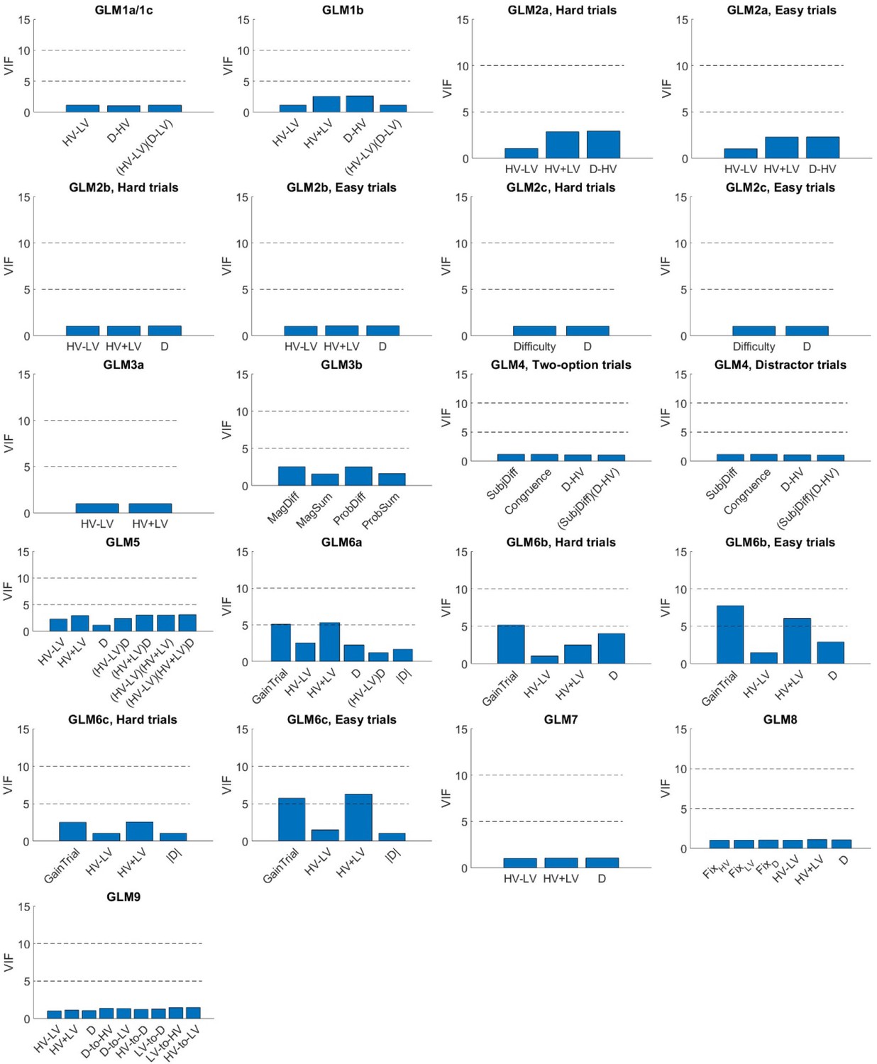
Variance inflation factor of each regressor.
Each plot shows the levels of variance inflation factor (VIF) of each regressor in the general linear models used.
Appendix 1—figure 1
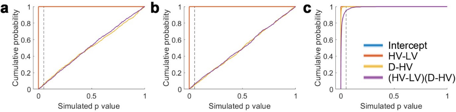
No clear indication of inflated statistical artefact in GLM1a.
GLM1a includes regressors HV-LV, D-HV and (HV-LV)(D–HV) to predict choice accuracy. (a) In Simulation 1, choice accuracy data was simulated using the effect size of HV-LV estimated by GLM1a from actual participants and assuming that the D-HV and (HV-LV)(D–HV) effects are absent. Then GLM1a was applied again to analyse the simulated choice accuracy data. In 1000 iterations, the chance of obtaining a significant effect (p<0.05; at the dashed line) from the HV-LV term is 100% (i.e. 0% Type II error; orange). For the D-HV and (HV-LV)(D–HV) terms, for which no effect is assumed, the chances of obtaining Type I errors are 5.6% and 5.1% respectively (yellow and purple respectively). (b) Simulation 2 is similar to Simulation 1, except that the effect size of HV-LV was estimated from the empirical data using a GLM that only includes the HV-LV term. (c) Simulation 3 assumes that HV-LV, D-HV and (HV-LV)(D–HV) effects are all present in the simulated choice accuracy data. The chances of obtaining a significant effect are 0%, 0.1% and 4.7% respectively. Note that in (a) and (b) the blue and orange lines overlap with each other; in (c) the blue, orange and yellow lines overlap with each other.
Appendix 3—figure 1
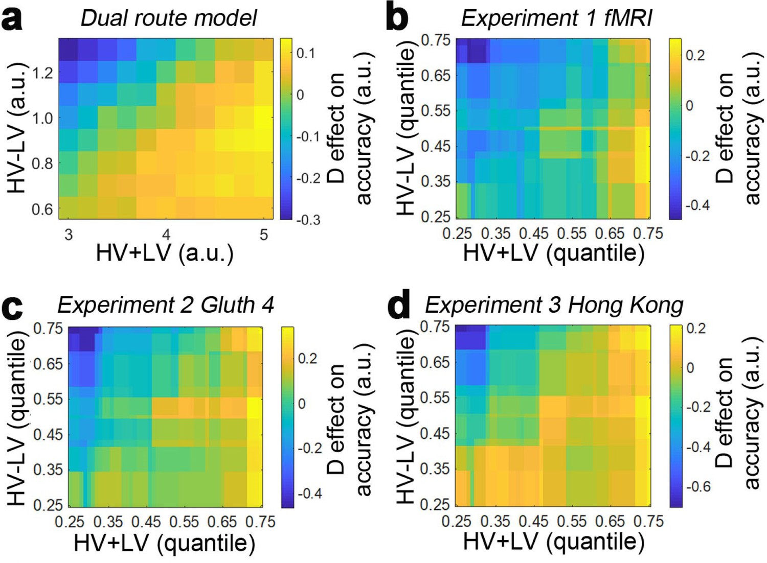
Distractor effects measured across the decision space.
As in Figure 1, the distractor effect (yellow = positive, blue = negative) is plotted across the decision space defined by difficulty (HV-LV) and the total value of the choosable options (HV+LV). Results are shown for (a) the dual route model, (b) Experiment 1 fMRI2014, (c) Experiment 2 Gluth4, (d) Experiment 3 Hong Kong.
Appendix 3—figure 2
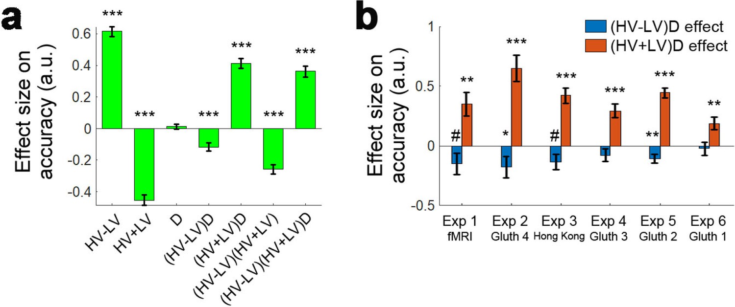
The distractor effect was modulated as a function of difficulty and the total value of the chooseable options.
(a) Here the data have been analysed with a more complete GLM (GLM5) including all main effects and two- and three-way interactions. Across all experiments the (HV-LV)D interaction is negative – the distractor has a positive effect on decision accuracy when decisions are difficult but a negative effect when decisions are easy. This resembles the effects illustrated in Figures 3–5. Moreover, across all experiments the (HV+LV)D interaction is positive – when the total value of the choosable options changed from large to small the distractor effect also changed from positive to negative. The divisive normalization model predicts that the negative impact of D is greatest when HV+LV is small (Figure 1) but its impact is reduced when HV+LV is large and so the positive distractor effect predicted by the interacting diffusion process model predominates when HV+LV is large. (b) The same two key interaction terms, (HV-LV)D and (HV+LV)D, indexing the positive distractor and divisive normalization effects are illustrated for each component experiment that was included in panel a. ***p<0.001. Error bars indicate standard error.
Additional files
-
Supplementary file 1
Supplementary tables.
(A) Regression coefficients estimated using the analysis procedures suggested by Gluth et al., 2018. (B) Simulation 1: testing the probabilities of Type I and II errors when distractor effects were assumed to be absent in the simulated choice data. (C) Simulation 2: an alternative approach for testing the probabilities of Type I and II errors when distractor effects were assumed to be absent in the simulated choice data. (D) Simulation 3: testing the probabilities of Type I and II errors when distractor effects were assumed to be present in the simulated choice data.
- https://cdn.elifesciences.org/articles/53850/elife-53850-supp1-v2.docx
-
Transparent reporting form
- https://cdn.elifesciences.org/articles/53850/elife-53850-transrepform-v2.docx
Download links
A two-part list of links to download the article, or parts of the article, in various formats.
Downloads (link to download the article as PDF)
Open citations (links to open the citations from this article in various online reference manager services)
Cite this article (links to download the citations from this article in formats compatible with various reference manager tools)
Consistent patterns of distractor effects during decision making
eLife 9:e53850.
https://doi.org/10.7554/eLife.53850


