Mechanics and kinetics of dynamic instability
- Paulson School of Engineering and Applied Sciences, Harvard University, United States
- Department of Modern Mechanics, University of Science and Technology of China, China
- IAT Chungu Joint Laboratory for Additive Manufacturing, Anhui Chungu 3D Institute of Intelligent Equipment and Industrial Technology, China
- Department of Physics, Harvard University, United States
- Department of Organismic and Evolutionary Biology, Harvard University, United States
Figures
Figure 1
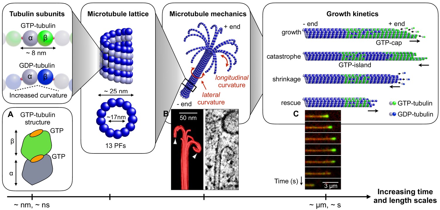
Connecting mechanical and kinetic aspects of MT dynamic instability across multiple time and length scales.
MTs are composed of tubulin heterodimers formed of α-tubulin and β-tubulin. Both α-tubulin and β-tubulin are bound to GTP, but only the GTP that is bound to a β-tubulin is hydrolysable (Nogales et al., 1998). When the tubulin dimer is part of the MT lattice, GTP hydrolysis increases the spontaneous longitudinal curvature along the dimer axis. This causes GDP-tubulin dimers to be less tightly bound in the MT lattice (Wang and Nogales, 2005; Alushin et al., 2014). In the scheme, GTP-tubulin dimers are shown in green, while GDP-tubulin dimers are shown in blue; dark color indicates β-tubulin and light colour indicates -tubulin. Tubulin dimers are connected head-to-tail into PFs. Typically, 13 such PFs align laterally to form the MT lattice, which is a long and hollow cylindrical shell with an outer diameter of approximately 25 nm and a thickness of about 5 nm (Mandelkow et al., 1986; Chrétien and Wade, 1991; Mitchison, 1993; Tilney et al., 1973). The mechanical stability/instability of the MT tube structure results from a competition between lateral and longitudinal curvatures. While MTs made of GTP-tubulin are relatively straight (about 5° per subunit), MTs made of GDP-tubulin tend to curve outward longitudinally at the plus end due to the longitudinal spontaneous curvature of GDP-tubulin dimers (about 12° per subunit) (Chrétien et al., 1995). Consequently, MTs consisting of GDP-tubulin (hydrolyzed MTs) tend to be mechanically less stable that their non-hydrolysed counterparts. The images show: (a) Schematic structure of an unhydrolyzed αβ-tubulin dimer with bound nucleotides highlighted in orange (Alushin et al., 2014). (b) EM image showing the characteristic shape of a depolymerising MT plus end, resembling a ram’s horn (VanBuren et al., 2005). (c) Sequence of TIRF microscopy images of a MT end illustrating the switching between phases of polymerisation and depolymerisation during dynamic instability; catastrophe is associated with the loss of the GTP-caps (green fluorescence is from a protein that is believed to associate with the GTP cap). (a) is adapted from Alushin et al. (2014); (b) is reproduced from Austin et al. (2005). (c) is reproduced from Duellberg et al. (2016) under the Creative Commons Attribution License CC-BY-4.0 (https://creativecommons.org/licenses/by/4.0/).
© 2005 Company of Biologists Ltd. All rights reserved. Panel B is reproduced from Austin et al. (2005) with permission. It is not covered by the CC-BY 4.0 licence and further reproduction of this panel would need permission from the copyright holder.
Figure 2
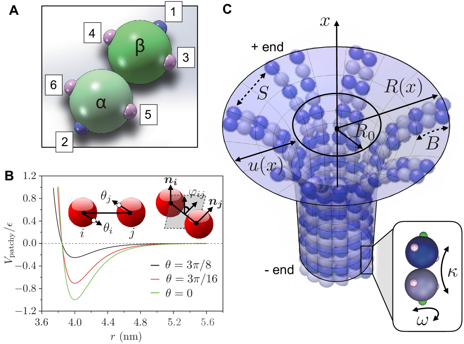
Definition of computer simulation and mechanical model.
(a) The GTP-tubulin subunit (-heterodimer) in our coarse-grained computer model. The blue patches (1 and 2) are longitudinal connecting points, while the pink patches (3 to 6) are lateral ones. This setup allows the dimer to curve inward along the MT longitudinal direction and outward laterally. The positions of the patches allow us to control the longitudinal and lateral curvatures of the subunit, giving a strong curvature (12°) to hydrolysed dimers and a weaker curvature (5°) to non-hydrolysed dimers. (b) The interaction potential between two patchy particles as a function of their centre-to-centre distance for and increasing . Inset: the bending angles and are defined as the angles between the centre-to-patch line and the centre-to-centre line; the twisting angle is defined by the projection of the normals and on the plane perpendicular to the centre-to-centre line. (c) Our mechanical model describes a MT as a continuous, thin elastic sheet. This is parameterised as a surface of revolution obtained by rotating the function along the MT long axis (-axis), where is the natural radius of the MT and describes the local deformation of the surface away from . We approximate lateral interaction potentials between tubulin subunits in neighbouring PFs by a set of spring potentials (springs with stiffness ). Bending of the PFs in the MT causes the connecting springs to stretch. This competition between bending energy and stretching energy determines the mechanical stability of MTs. Inset: hydrolysed tubulin dimers curve naturally in two directions as described by the longitudinal and lateral spontaneous curvatures and , respectively.
Figure 3
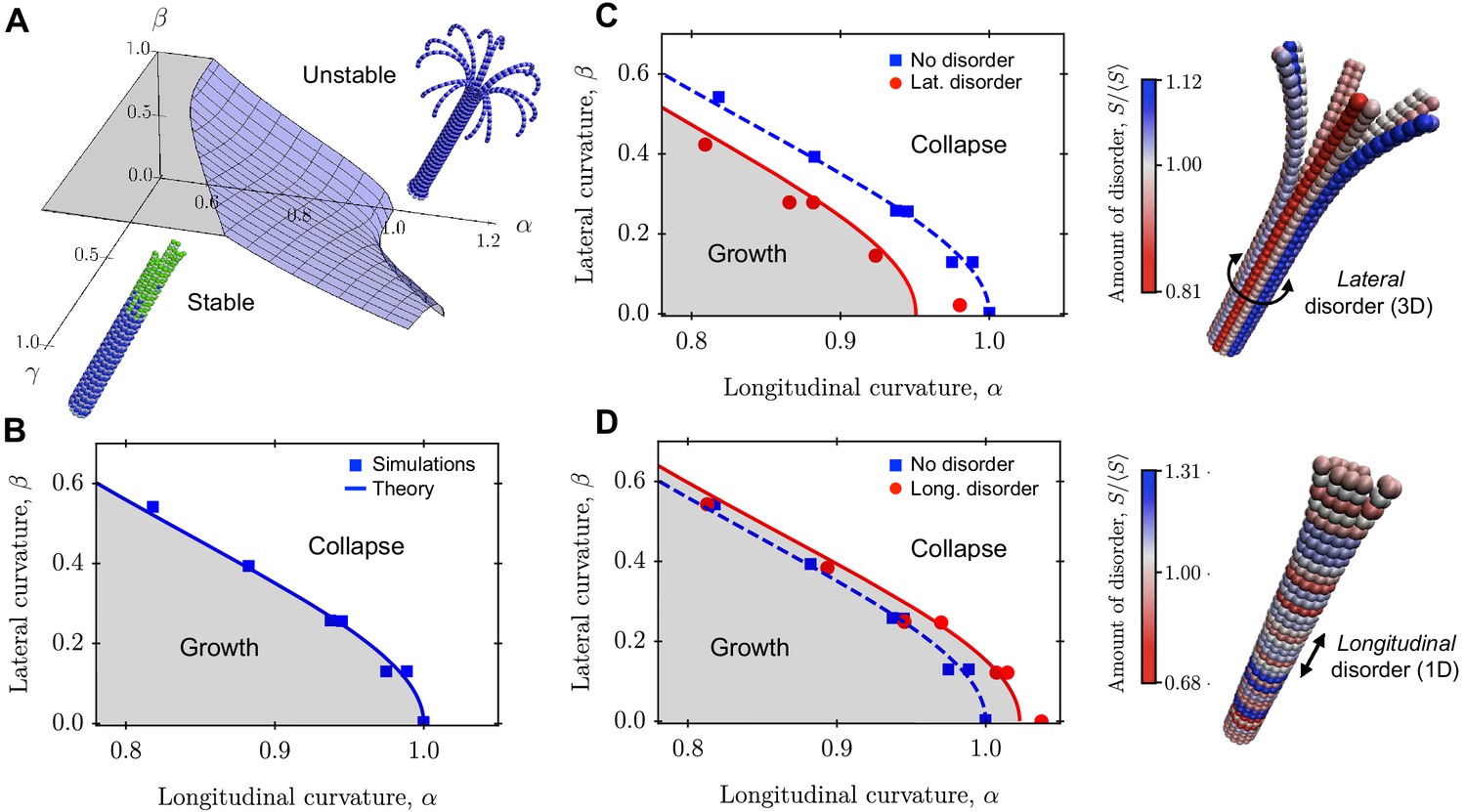
Role of lateral and longitudinal curvatures in mechanical stability of a 3D MT in the absence and presence of quenched disorder.
(a) Schematic phase diagram for mechanical stability/instability with three axes (two mechanical axes and one kinetic axis): longitudinal curvature parameter , lateral curvature parameter , and ratio of growth rate to hydrolysis rate . (b) 2D phase diagram separating regions of mechanically stable and unstable MTs as a function of and . Data points are from computer simulations and the solid line is the prediction of Equation 13. (c)-(d) Implementation of lateral (c) and longitudinal (d) disorder at the level of the spring stiffness in our coarse-grained computer model. The data points are simulation results and the solid lines are fits to Equation 16 and Equation 17. The data show that lateral disorder acts to destabilise MTs mechanically (c), while longitudinal disorder strengthens MTs (d). In both cases, disorder was generated using the distribution of spring constants in Equation 14 with , that is the disorder parameter was . The amount disorder of each tubulin subunit represents the average value of the relative stiffness of its two lateral interactions. See Videos 1–4 for movies illustrating the mechanical stability of a MT with and without quenched disorder (see Videos 1–4).
-
Figure 3—source data 1
This spreadsheet contains the data for Figure 3B,C and D.
- https://cdn.elifesciences.org/articles/54077/elife-54077-fig3-data1-v1.xls
Figure 4
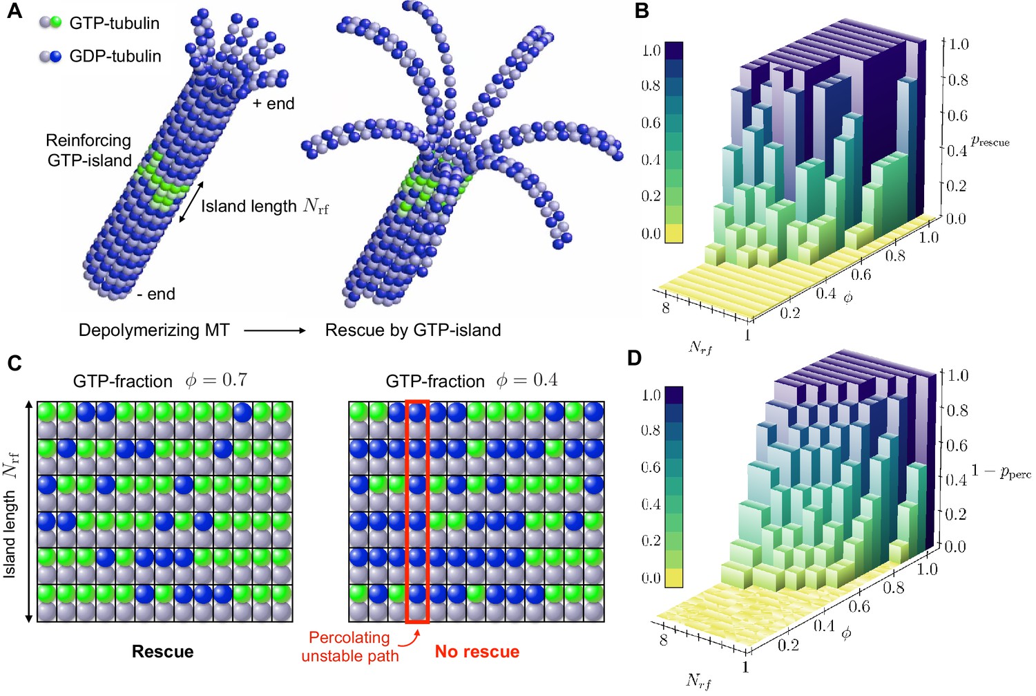
Role of disordered GTP-islands in rescue.
(a) Schematics showing the rescue of a depolymerising MT reinforced by a disordered GTP-tubulin island. In this example, the length of the reinforcing island is and the GTP-island consists of 20 GTP-tubulin dimers, which corresponds to a GTP-fraction of (see Video 5). (b) Simulated rescue probability by GTP-islands as a function of GTP-fraction and reinforcing island length . The rescue probability was estimated by repeating simulations six to ten times for each pair and . (c) Percolation model for the role of disordered reinforcing GTP-islands on MT rescue. (d) Simulated site percolation on a square lattice with dimensions as a function of GTP-fraction and island length . The probability of percolation was obtained by averaging over 103 realisations for each pair and .
-
Figure 4—source data 1
This spreadsheet contains the data for Figure 4B.
- https://cdn.elifesciences.org/articles/54077/elife-54077-fig4-data1-v1.xls
-
Figure 4—source data 2
This spreadsheet contains the data for Figure 4D.
- https://cdn.elifesciences.org/articles/54077/elife-54077-fig4-data2-v1.xls
Appendix 1—figure 1
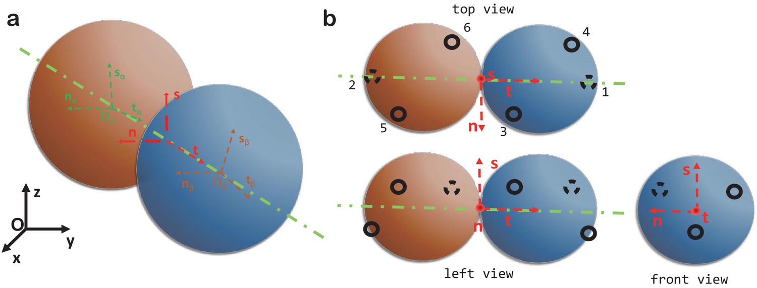
Computer model.
(a) The local coordinate systems of a dimer. (b) Top, left and front views of two spheres forming a dimer and the six patchy points.
Appendix 1—figure 2
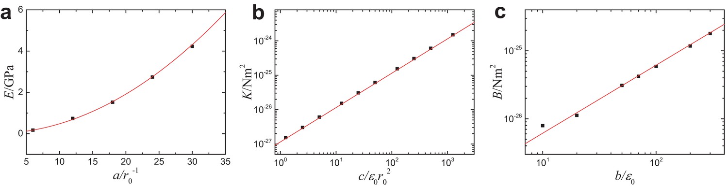
Mesoscopic mechanical properties of MTs as functions of the parameters in the coarse-grained simulations model.
(a) Young’s modulus vs , (b) torsional rigidity vs and (c) bending stiffness vs . Solid lines correspond to the theoretical predictions (see Equation 7 in Section ’Computational model’ of main text), and are in good agreement with the computer simulations.
Appendix 2—figure 1

Continuum elastic shell model of microtubule.
(a) To describe the curvature energy, MTs are modelled as thin elastic surfaces of revolution obtained by rotating the function along the MT long axis ( axis). is the natural radius of the MT. (b) Neighbouring PFs within the MT are connected by Hookean springs with stiffness .
Appendix 2—figure 2
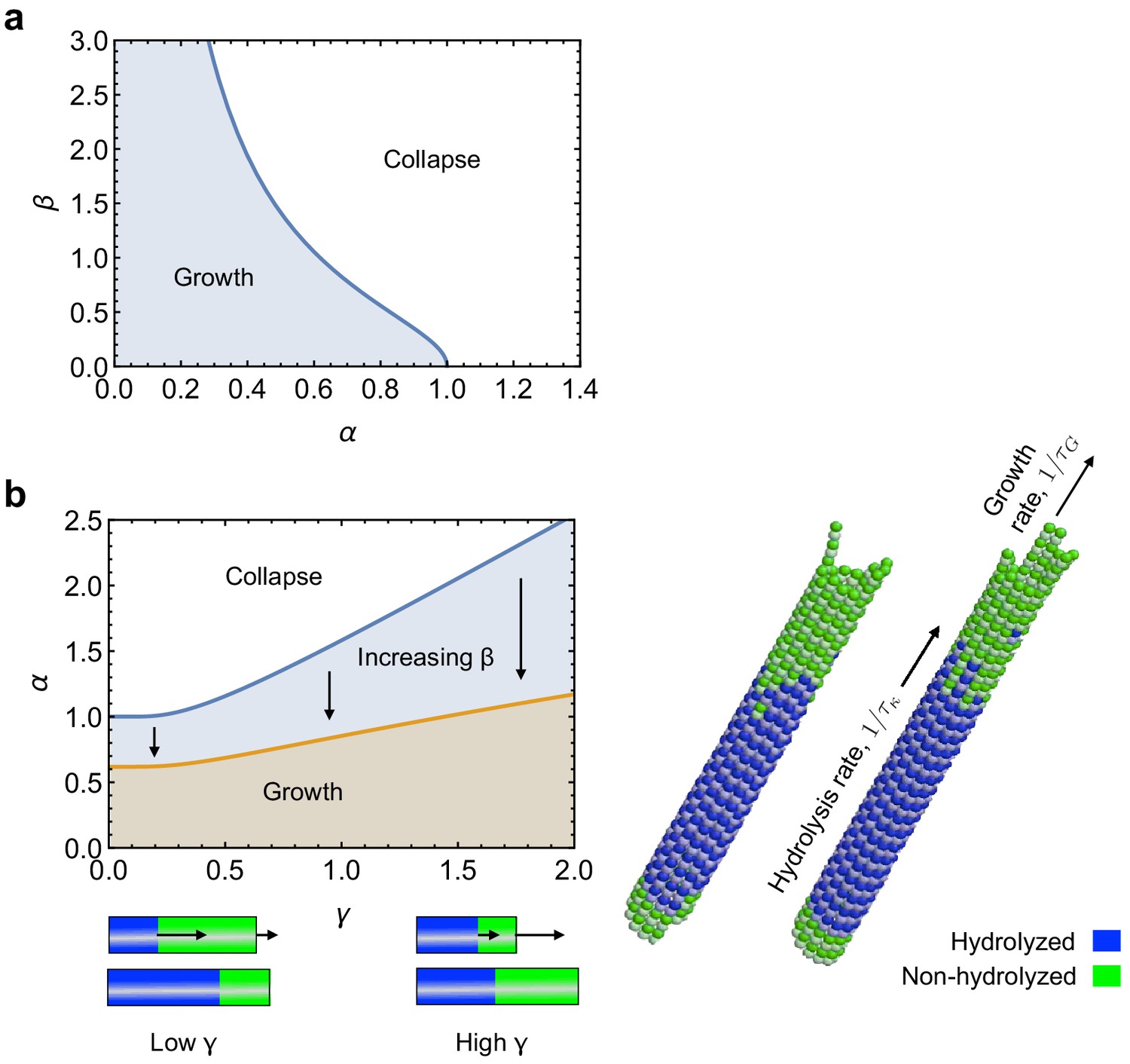
Role of kinetics on mechanical stabillity of MTs.
(a) Phase diagram for mechanical stability of 3D MTs, as described by Equation 50. (b) Effect of the relative rates of tubulin hydrolysis and MT growth () on mechanical stability of MTs, as described by Equation 62. See: link to Videos 1 and 2.
Appendix 2—figure 3
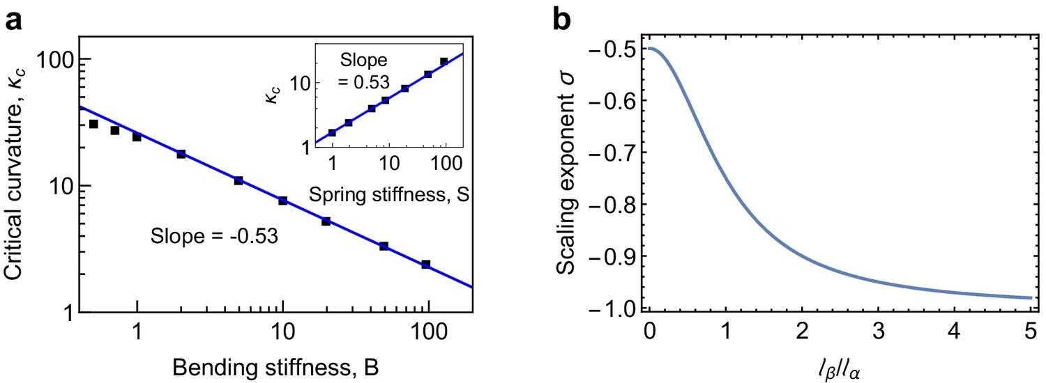
Scaling behaviour of critical curvature.
(a) Scaling behavior of the critical longitudinal curvature with bending stiffness and spring stiffness (inset). The scaling relationship over the range of and values investigated in the simulations is found to be , in agreement with the predictions of Equation 55. (b) Scaling exponent (Equation 55) as a function of interpolates between the limits for and for .
-
Appendix 2—figure 3—source data 1
This spreadsheet contains the data for Appendix 2—figure 3a.
- https://cdn.elifesciences.org/articles/54077/elife-54077-app2-fig3-data1-v1.xls
Appendix 2—figure 4
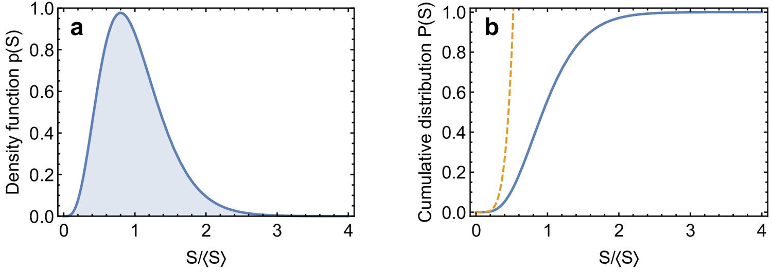
Gamma distribution.
(a) Gamma distribution Equation 64 with . (b) Cumulative probability distribution for the Gamma distribution, Equation 70, and low value-tail, Equation 72 (dashed line).
Videos
Video 1
MT growth and hydrolysis kinetics.
This movie shows the interplay between MT growth kinetics (we focus here only on the addition of GTP-tubulin subunits at the plus end) and the subsequent hydrolysis of the incorporated subunits in the older parts of the MT. The interplay between growth and hydrolysis can be seen in the emergence of a growing front and a hydrolysis front that move with different speed. In this case, the hydrolysis front does not catch up with the growth front at the plus end, yielding a stabilising GTP-cap and a mechanically stable MT configuration for the entire duration of the simulation. The growth rate is steps−1, while the probability of hydrolysis for each dimer is given by , where steps−1 is the rate of hydrolysis. Note the separation of timescales between MT growth and subunit hydrolysis (). To keep the helical structure stable, we use the following parameters , and , while the other mechanical parameters are the same as listed in Table 1.
Video 2
MT catastrophe.
This movie shows the interplay between MT growth and subunit hydrolysis. The rate of hydrolysis is steps−1 while the growth rate is decreasing from steps−1 to steps−1. Hydrolysis destroys the GTP-cap of MT and causes catastrophe. The mechanical parameters are the same as in Video 1.
Video 3
Role of lateral quenched disorder in MT mechanical stability.
This movie illustrates the stability of a MT in the presence of lateral disorder in the spring stiffness , which describes the strength of lateral contacts between PFs. Note that lateral disorder causes the MT to be mechanically unstable along directions with weakest lateral bonds (the MT ‘cut opens’ along these weak directions). The color code indicates the local value of for each subunit, which is obtained by averaging over the relative stiffness of its two lateral bonds (drawn from the Gamma-distribution (14) with ). The simulation parameters are the same as listed in Table 1, except that we set for all tubulin dimers.
Video 4
Role of longitudinal quenched disorder in MT mechanical stability.
This movie illustrates the stability of a MT in the presence of longitudinal disorder in the spring stiffness . Note that the MT is in this case mechanically more stable than in the presence of lateral disorder. This is because longitudinal disorder leads to the presence of ‘rings’ of strong bonds that prevent the MT from peeling off completely. The simulation parameters are the same as in Video 3.
Video 5
MT rescue by disordered GTP-island.
This movie illustrates the successful rescue of a depolymerising MT by a disordered GTP-island placed along the MT lattice. The mechanical parameters in this case are the same as in Video 1.
Tables
Table 1
Values of parameters used in our coarse-grained simulations.
| Parameter | Value | Description |
|---|---|---|
| 4 nm | Equilibrium distance between tubulin monomers | |
| 7.665 × 10⁻²⁰J | Potential energy depth for longitudinal interactions | |
| 5° or 12° | Angle between α-tubulin and β-tubulin within a GTP- or GDP-dimer | |
| 3° | See Equations 24-29 | |
| 103.45° or 90° | See Equations 24-29 | |
| 13.8° | See Equations 24-29 | |
| Longitudinal size of tubulin dimers | ||
| Lateral size of tubulin dimers | ||
| 20/ | Parameters that control longitudinal and lateral stretching stiffness | |
| Parameter that controls longitudinal bending stiffness | ||
| Parameter that controls lateral bending stiffness | ||
| Parameter controls longitudinal twisting stiffness | ||
| Parameter that controls lateral twisting stiffness | ||
| Potential energy depth for longitudinal interactions | ||
| 0.0906ε0 | Potential energy depth for lateral interactions |
Additional files
-
Transparent reporting form
- https://cdn.elifesciences.org/articles/54077/elife-54077-transrepform-v1.pdf
-
Appendix 2—figure 3—source data 1
This spreadsheet contains the data for Appendix 2—figure 3a.
- https://cdn.elifesciences.org/articles/54077/elife-54077-app2-fig3-data1-v1.xls
Download links
A two-part list of links to download the article, or parts of the article, in various formats.
Downloads (link to download the article as PDF)
Open citations (links to open the citations from this article in various online reference manager services)
Cite this article (links to download the citations from this article in formats compatible with various reference manager tools)
Mechanics and kinetics of dynamic instability
eLife 9:e54077.
https://doi.org/10.7554/eLife.54077


