Global sleep homeostasis reflects temporally and spatially integrated local cortical neuronal activity
- Department of Physiology, Anatomy and Genetics, University of Oxford, United Kingdom
- Nuffield Department of Clinical Neurosciences, University of Oxford, United Kingdom
- Institute of Pharmacology and Toxicology, University of Zurich, Switzerland
- The KEY Institute for Brain-Mind Research, Department of Psychiatry, Psychotherapy and Psychosomatics, University Hospital of Psychiatry, Switzerland
Figures
Figure 1
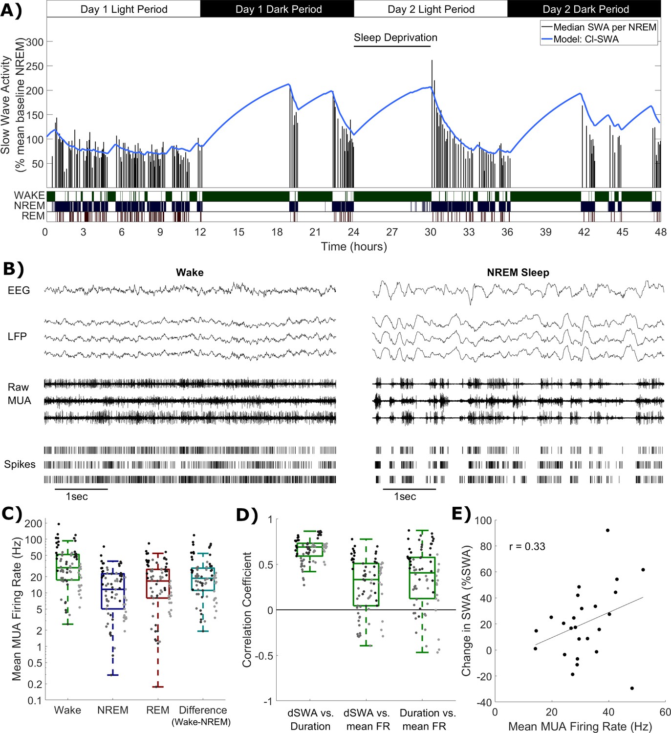
Cortical spike firing patterns are associated with the dynamics of Process S.
(A) An example of the classical state-based Process S model (blue) describing the dynamics of frontal EEG SWA (median per NREM sleep episode, black bars) over 48 h in one representative animal. Sleep deprivation occurred as indicated at light onset of the second day and lasted 6 h. Scored vigilance states are also shown. (B) An example of frontal electroencephalogram (EEG), primary motor cortical local field potentials (LFP), corresponding raw signal with multi-unit activity (MUA) and detected spikes, in representative segments of waking and NREM sleep. Slow waves and synchronous spiking off periods are visible in NREM sleep but not in wakefulness. The y-scale is the same for both wake and NREM sleep plots. (C) The distribution (log scale) of mean firing rates during wake, NREM and REM sleep over all animals and channels, in addition to the difference in mean firing rates in wake compared to NREM sleep (all are positive, reflecting higher firing in wake). Points indicate channels grouped by animal (left to right), but boxplots reflect channels from all animals treated as one population. (D) Distribution of correlation coefficients, calculated within each single channel, between wake episode duration (Duration), the change in slow wave activity (dSWA), and mean firing rate (mean FR). Points indicate channels grouped by animal (left to right), but boxplots reflect channels from all animals treated as one population. (E) An example scatter plot of the correlation between the change in median SWA from one NREM episode to the next and the mean firing rate during the intervening period of wakefulness. This channel is representative because it has the median correlation coefficient of all channels.
-
Figure 1—source data 1
Slow wave activity, firing rate and vigilance state time series data.
- https://cdn.elifesciences.org/articles/54148/elife-54148-fig1-data1-v1.zip
Figure 2
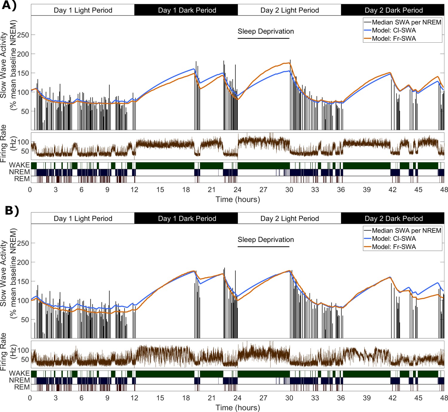
Slow wave activity dynamics at the LFP level can be modelled using multi-unit spiking information.
(A) An example from one representative animal modelling the SWA averaged over all LFP channels, of both the classical model (blue) and novel firing-rate-based model (orange), calculated from the firing rate also averaged over all LFP channels (brown). (B) An example of both models applied to the SWA of a single LFP channel, which came from the same animal as used in A.
Figure 3 with 1 supplement
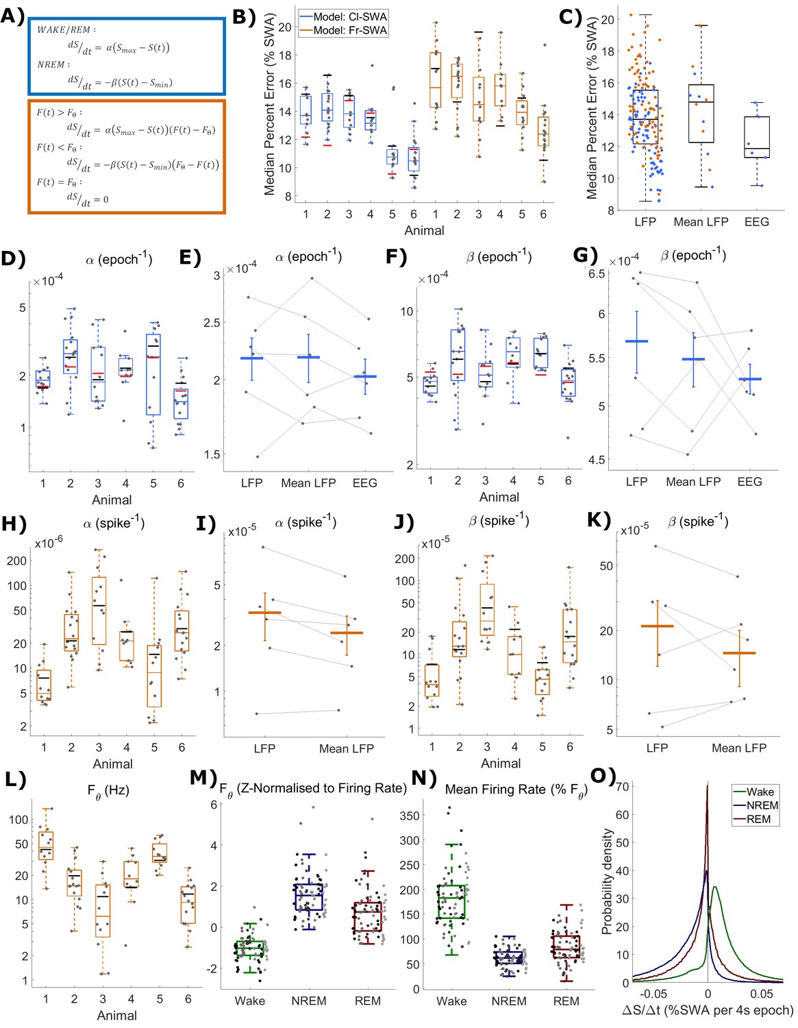
The fit quality and parameters for both classical and firing-rate-based models of LFP SWA.
(A) Equations for the classic state-based model (blue) and novel firing-rate-based model (orange). (B) For each animal, the distribution over channels of the median absolute difference between the model and empirical SWA, expressed as a percentage of empirical SWA, for both classic and firing-rate-based models. Black lines indicate the values obtained from modelling the averaged LFP SWA and firing rate over all channels within an animal and the red lines give the parameter value obtained from the model applied to the frontal EEG SWA of that animal. (C) The same median percent error, grouped over animals and models, separately showing errors at the level of single LFP, averaged LFP and EEG. (D–K) The distribution (log scale) of values estimated for α and β rate parameters in the classic model (blue) and in the firing-rate-based model (orange). Parameter values are first presented with boxplots plotted separately for each animal (D, F, H, J), then are additionally shown grouped by level of analysis (E, G, I, K), including single LFP channel, mean of LFPs, or (E and I only) frontal EEG. Vertical lines indicate the standard error of the group mean and grey lines connect points derived from the same animal across groups. (L) The distribution of the final optimised value for the firing rate set point parameter (Fθ) of the firing-rate-based model grouped by animal. (M) The same values z-normalised to the distribution of firing rates within wake, NREM and REM sleep. (N) The distribution of mean firing rate in wake, NREM and REM sleep, expressed as a percentage of the firing rate set point parameter (Fθ). Points indicate channels grouped and coloured by animal, but boxplots reflect all channels treated as one population. (O) The distribution of the change in Process S (ΔS/Δt) from one 4 s time step to the next derived from the Fr-SWA model in wake, NREM sleep and REM sleep. All mice, channels and time are pooled.
-
Figure 3—source data 1
Process S time series and parameters based on SWA for classic and novel models.
- https://cdn.elifesciences.org/articles/54148/elife-54148-fig3-data1-v1.zip
Figure 3—figure supplement 1
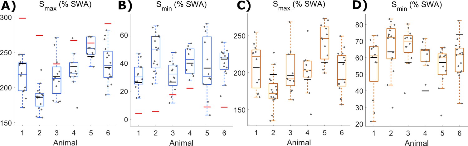
Values for Smax and Smin parameters in Process S models derived from SWA.
(A) The distribution of values estimated for Smax and (B) Smin parameters in Process S models derived from SWA with the classic model and (C-D) with the firing-rate-based model, with boxplots plotted separately for each animal. The black lines indicate the values obtained from modelling the averaged LFP SWA and firing rate over all channels within an animal. Additionally, the red lines (in A and B only) give the parameter value obtained from the model of the frontal EEG SWA of the corresponding animal.
Figure 4
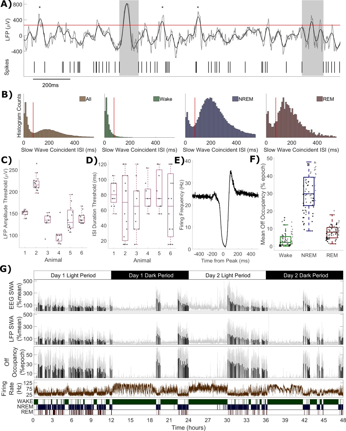
Definition of off periods and off occupancy.
(A) An example section of LFP (raw in grey, 0.5–6 Hz filtered in black) and simultaneous MUA spikes. During this time window, the filtered LFP crosses the amplitude threshold (265 μV for this channel, red line) five times. The MUA inter-spike interval aligned to two of these peaks exceeds the duration threshold (85 ms for this channel) and so two off periods are detected (grey boxes). ISIs aligned to the other three out of five crossings (asterisks) are too short to be considered off periods. (B) Histograms of multi-unit inter-spike intervals aligned with detected slow waves (0 = peak of slow wave) for this example channel. The four plots show, from left to right, ISIs over the whole recording and ISIs separately during wake, NREM and REM sleep only. The ISI duration threshold (red line) is selected using the histogram of all ISIs (leftmost) at the minimum between the two modes (and shown for comparison in the wake, NREM and REM sleep panels). (C) The distribution of LFP amplitude and (D) ISI duration threshold values used for definition of off periods for each channel, with boxplots plotted separately for each animal. (E) The mean multi-unit firing rate over a period of 1 s centred on the peak of detected slow waves, calculated over all slow waves within one example channel with a resolution of 1 ms. (F) Distributions of mean off occupancy (%) for all channels averaged over wake, NREM and REM sleep. Points indicate channels grouped by animal (left to right), but boxplots reflect all channels treated as one population. (G) Off occupancy is shown alongside EEG and LFP SWA for an example channel over 48 h. Traces represent these values calculated at 4 s resolution (light grey), in addition to the median value per NREM sleep episode, as used for model fitting (black bars). Firing rate (brown) and scored vigilance states are also shown.
-
Figure 4—source data 1
Off occupancy time series and off period detection parameters.
- https://cdn.elifesciences.org/articles/54148/elife-54148-fig4-data1-v1.zip
Figure 5 with 1 supplement

Process S is reflected in an LFP channel’s off occupancy and its dynamics are described well by both state-based and firing-rate-based models.
(A) An example of the novel model based on firing rates and off occupancy (purple), and the classic state-based model (blue), with optimised parameters describing the dynamics of off occupancy (median per NREM episode, black bars) over 48 h. Sleep deprivation occurred as indicated at light onset of the second day and lasted 6 h. Firing rate (brown), off occupancy (value per 4 s epoch, grey) and scored vigilance states are also shown. (B) Equations for the classic state-based model (blue) and firing-rate-and-off-occupancy-based model for off occupancy (purple). (C) For each animal, the distribution over channels of the median difference between the model and empirical off occupancy, expressed as a percentage of the off occupancy, for both classic and firing-rate-based models. (D) The distribution of values of the change in Process S (ΔS/Δt) from one 4 s time step to the next derived from the Fr-Off model in wake, NREM sleep and REM sleep. All mice, channels and time are pooled. (E–F) The distribution of optimised values used for the rate parameters in the classic model and (G-H) the firing rate model, with boxplots plotted separately for each animal.
-
Figure 5—source data 1
Process S time series and parameters based on off occupancy for classic and novel models.
- https://cdn.elifesciences.org/articles/54148/elife-54148-fig5-data1-v1.zip
Figure 5—figure supplement 1
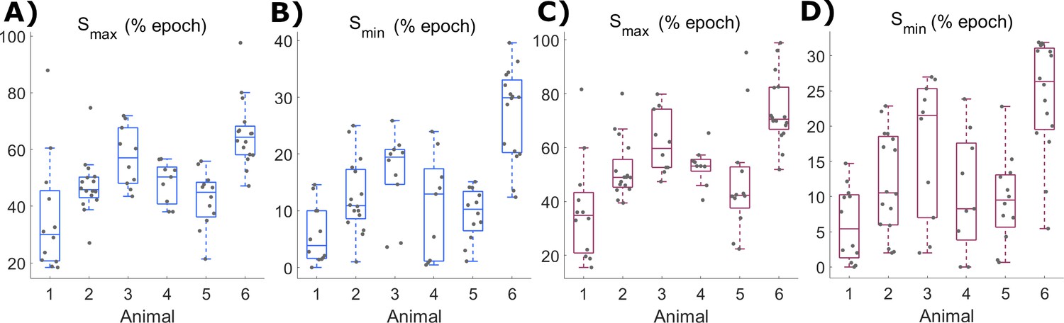
Values for Smax and Smin parameters in Process S models derived from off occupancy.
(A) The distribution of values used for Smax and (B) Smin parameters in Process S models derived from off occupancy with the classic model and (C-D) with the firing-rate-based model, with boxplots plotted separately for each animal.
Figure 6 with 1 supplement
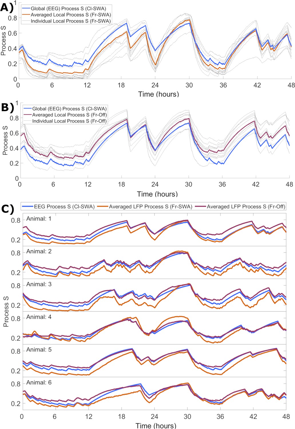
The time course of local activity-derived Process S averaged across channels resembles Process S derived from the EEG and sleep-wake history.
(A) The time course of Process S shown for one representative animal using the classical EEG-based model (blue), alongside average (orange) and individual channel (grey) Processes S derived from activity-dependent models of all individual LFP channels applied to SWA. (B) The same, except that Process S corresponding to individual channels (grey) and their average (purple) are derived from off periods. Note that the model in blue remains Cl-SWA, as off periods cannot be derived from the EEG. (C) Process S derived from applying the Cl-SWA model to frontal EEG (blue) and the mean Process S derived from applying Fr-SWA (orange) and Fr-Off (purple) to all individual channels. The results are shown for each of the six animals analysed. In all panels, all Process S time series are normalised between 0 to 1 relative to individual Smin and Smax values for fair comparison.
Figure 6—figure supplement 1
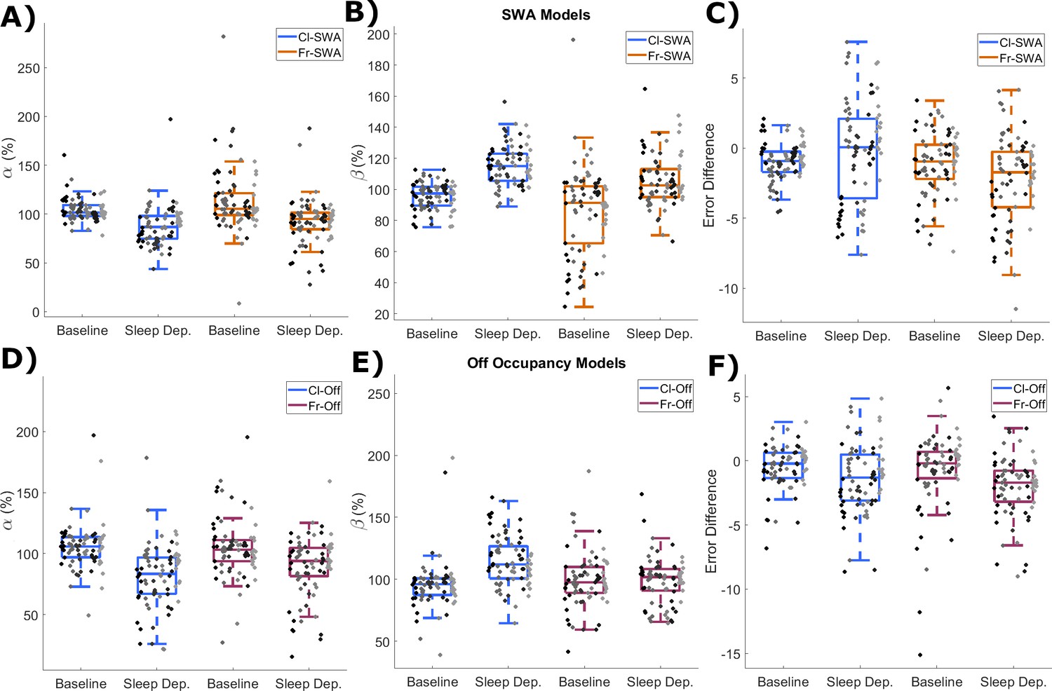
Cross-validation of parameter estimation.
(A) The values of the rate parameters α, and (B) β, obtained by algorithmic optimisation fitting to data from only the baseline or sleep deprivation day. For normalisation, values are expressed as a percentage of the original value obtained using the semi-automated approach (see Materials and methods). (C) The difference in the median percent error (E*) obtained from Process S with rate parameters optimised on either the baseline or sleep deprivation day from that obtained using the original semi-automated selected parameters. Negative values reflect improved fits. All values are shown for both classic (blue) and firing-rate-based (orange) models applied to SWA-derived Process S. (D–F) The same variables are shown for the models based on off occupancy using both classic (blue) and firing-rate-based (purple) models. Statistical analysis was performed for each variable by a three-factor ANOVA. (A) Day: F(1, 293)=56.1, p=8.1×10⁻¹³; Model: F(1, 293)=6.8, p=9.7×10⁻³; Animal: F(5, 293)=1.4, p=0.23; Day x Model: F(5, 293)=0.6, p=0.43; Day x Animal: F(5, 293)=4.8, p=3.5×10⁻⁴; Model x Animal: F(1, 293)=2.5, p=0.033; three-way ANOVA). (B) Day: F(1, 293)=110.9, p=3.3×10⁻²²; Model: F(1, 293)=28.9, p=1.6×10⁻⁷; Animal: F(5, 293)=0.7, p=0.60; Day x Model: F(5, 293)=0.1, p=0.98; Day x Animal: F(5, 293)=11.1, p=8.3×10⁻¹⁰; Model x Animal: F(5, 293)=11.6, p=7.4×10⁻⁴; three-way ANOVA). (C) Day: F(1, 293)=4.37, p=0.038; Model: F(1, 293)=16.3, p=7.1×10⁻⁵; Animal: F(5, 293)=17.3, p=5.3×10⁻¹⁵; Day x Model: F(1, 293)=2.1, p=0.064; Day x Animal: F(5, 293)=24.5, p=1.4×10⁻²⁰; Model x Animal: F(1, 293)=3.6, p=3.9×10⁻³; three-way ANOVA). (D) Day: F(1, 281)=48.2, p=2.6×10⁻¹¹; Model: F(1, 281)=2.6, p=0.11; Animal: F(5, 281)=2.6, p=0.027; Day x Model: F(5, 281)=3.2, p=0.077; Day x Animal: F(5, 281)=2.9, p=0.014; Model x Animal: F(1, 281)=0.8, p=0.54; three-way ANOVA). (E) Day: F(1, 281)=16.8, p=5.4×10⁻⁵; Model: F(1, 281)=4.6, p=0.033; Animal: F(5, 281)=0.8, p=0.50; Day x Model: F(5, 281)=13.0, p=3.7×10⁻⁴; Day x Animal: F(5, 281)=6.0, p=2.7×10⁻⁵; Model x Animal: F(1, 281)=1.2, p=0.31; three-way ANOVA). (F) Day: F(1, 281)=15.9, p=8.4×10⁻⁵; Model: F(1, 281)=1.4, p=0.25; Animal: F(5, 281)=7.5, p=1.2×10⁻⁶; Day x Model: F(5, 281)=0.3, p=0.56; Day x Animal: F(5, 281)=2.6, p=0.028; Model x Animal: F(1, 281)=0.8, p=0.58; three-way ANOVA).
Additional files
-
Source code 1
Process S model parameter optimisation code.
- https://cdn.elifesciences.org/articles/54148/elife-54148-code1-v1.zip
-
Transparent reporting form
- https://cdn.elifesciences.org/articles/54148/elife-54148-transrepform-v1.pdf
Download links
A two-part list of links to download the article, or parts of the article, in various formats.
Downloads (link to download the article as PDF)
Open citations (links to open the citations from this article in various online reference manager services)
Cite this article (links to download the citations from this article in formats compatible with various reference manager tools)
Global sleep homeostasis reflects temporally and spatially integrated local cortical neuronal activity
eLife 9:e54148.
https://doi.org/10.7554/eLife.54148


