Using the past to estimate sensory uncertainty
- Psychology Department, Durham University, United Kingdom
- Department of Psychiatry and Psychotherapy, University of Tübingen, Germany
- Department of Psychology, Friedrich-Alexander University Erlangen-Nuernberg, Germany
- Centre for Computational Neuroscience and Cognitive Robotics, University of Birmingham, United Kingdom
- Max Planck Institute for Intelligent Systems, Germany
- European Molecular Biology Laboratory, Genome Biology Unit, Germany
- Division of Computational Genomics and Systems Genetics, German Cancer Research Center (DKFZ), Heidelberg, Germany, Germany
- Donders Institute for Brain, Cognition and Behaviour, Radboud University, Netherlands
Figures
Figure 1 with 1 supplement
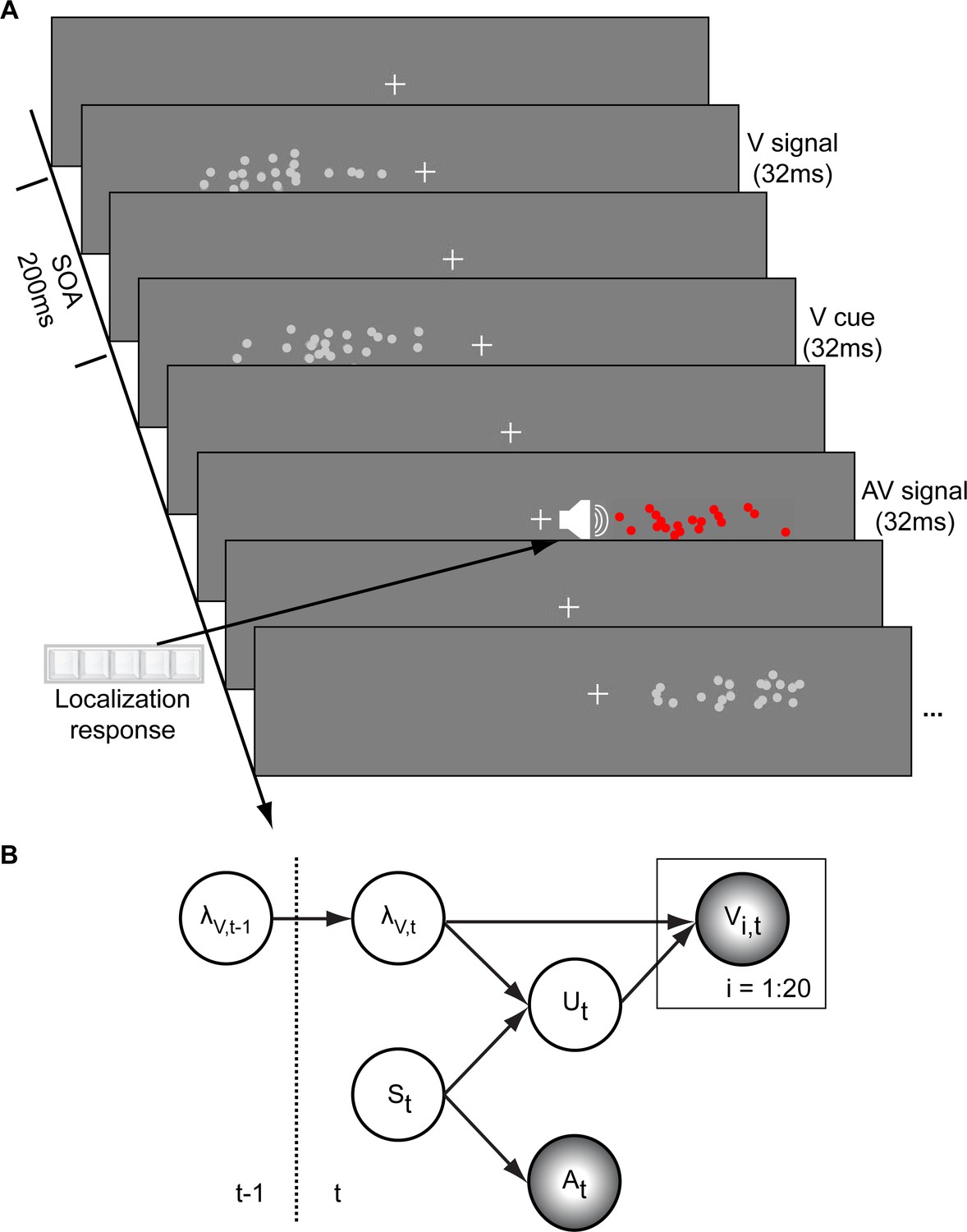
Audiovisual localization paradigm and Bayesian causal inference model for learning visual reliability.
(A) Visual (V) signals (cloud of 20 bright dots) were presented every 200 ms for 32 ms. The cloud’s location mean was temporally independently resampled from five possible locations (−10°, −5°, 0°, 5°, 10°) with an inter-trial asynchrony jittered between 1.4 and 2.8 s. In synchrony with the change in the cloud’s mean location, the dots changed their color and a sound was presented (AV signal) which the participants localized using five response buttons. The location of the sound was sampled from the two possible locations adjacent to the visual cloud’s mean location (i.e. ±5° AV spatial). (B) The generative model for the Bayesian learner explicitly modeled the potential causal structures, that is whether visual (Vi) signals and an auditory (A) signal were generated by one common audiovisual source St, that is C = 1, or by two independent sources SVt and SAt, that is C = 2 (n.b. only the model component for the common source case is shown to illustrate the temporal updating, for complete generative model, see Figure 1—figure supplement 1). Importantly, the reliability (i.e. 1/variance) of the visual signal at time t (λt) depends on the reliability of the previous visual signal (λt-1) for both model components (i.e. common and independent sources).
Figure 1—figure supplement 1

Generative model for the Bayesian learner.
The Bayesian Causal Inference model explicitly models whether auditory and visual signals are generated by one common (C = 1) or two independent sources (C = 2) (for further details see Körding et al., 2007). We extend this Bayesian Causal Inference model into a Bayesian learning model by making the visual reliability (, i.e. the inverse of uncertainty or variance) of the current trial dependent on the previous trial.
Figure 2 with 1 supplement
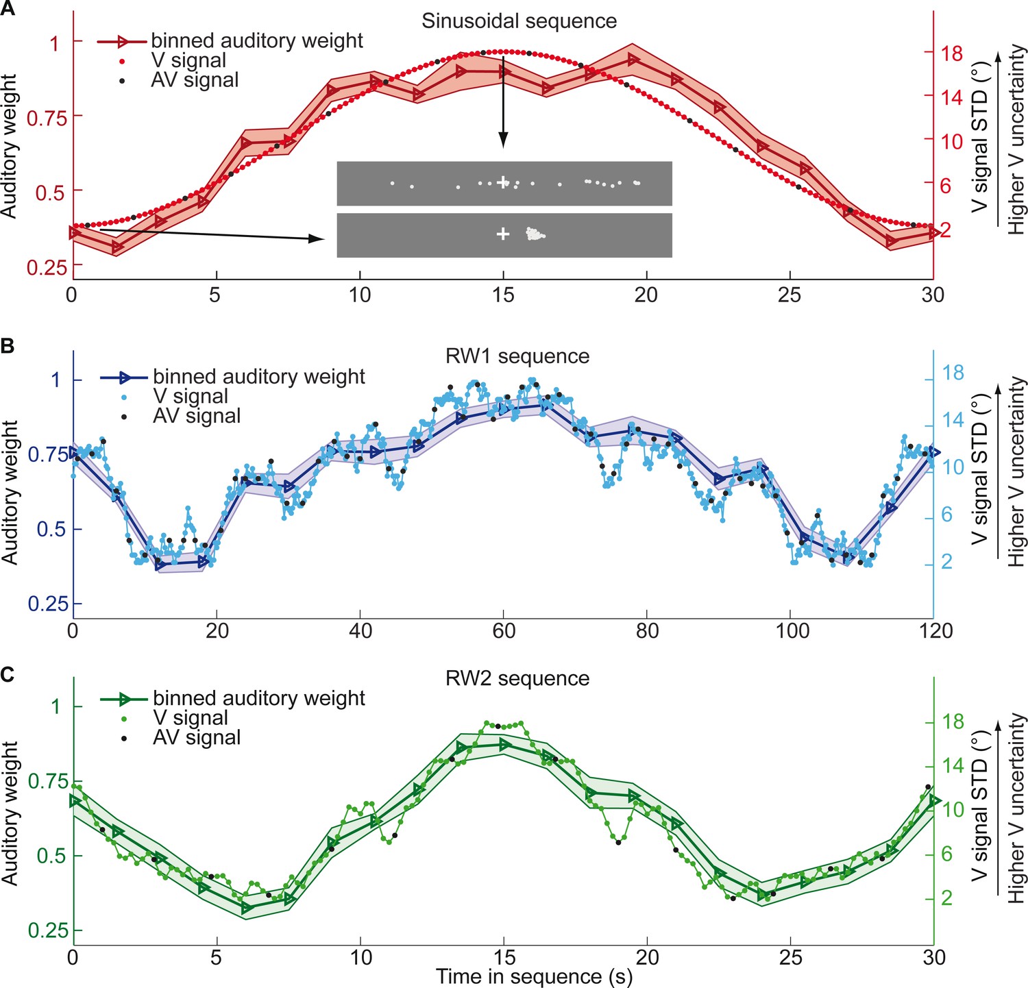
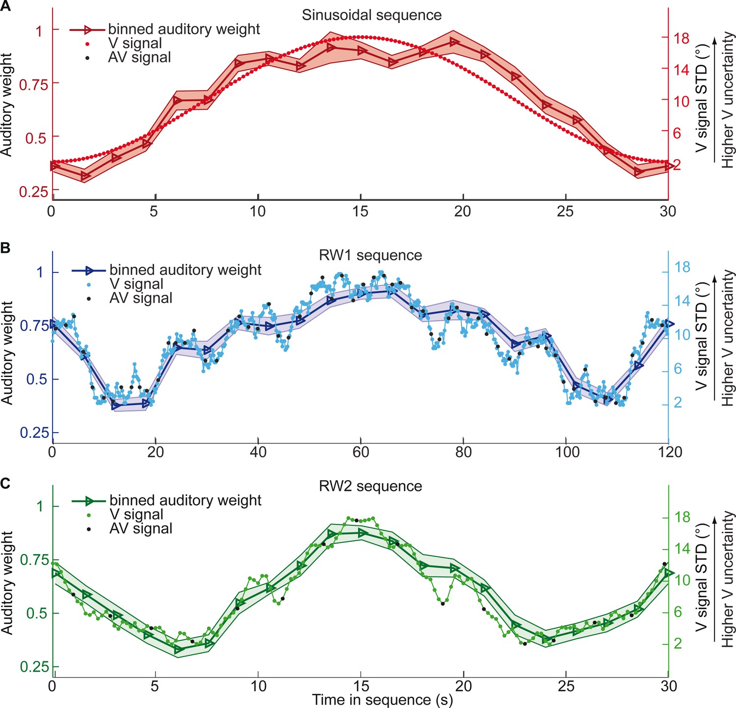
Time course of visual noise and relative auditory weights for continuous sequences of visual noise.
The visual noise (i.e. STD of the cloud of dots, right ordinate) and the relative auditory weights (mean across participants ± SEM, left ordinate) are displayed as a function of time. The STD of the visual cloud was manipulated as (A) a sinusoidal (period 30 s, N = 25), (B) a random walk (RW1, period 120 s, N = 33) and (C) a smoothed random walk (RW2, period 30 s, N = 19). The overall dynamics as quantified by the power spectrum is faster for RW2 than RW1 (peak in frequency range [0 0.2] Hz: Sinusoid: 0.033 Hz, RW1: 0.025 Hz, RW2: 0.066 Hz). The RW1 and RW2 sequences were mirror-symmetric around the half-time (i.e. the second half was the reversed first half). The visual clouds were re-displayed every 200 ms (i.e. at 5 Hz). The trial onsets, that is audiovisual (AV) signals (color change with sound presentation, black dots), were interspersed with an inter-trial asynchrony jittered between 1.4 and 2.8 s. On each trial observers located the sound. The relative auditory weights were computed based on regression models for the sound localization responses separately for each of the 20 temporally adjacent bins that cover the entire period within each participant. The relative auditory weights vary between one (i.e. pure auditory influence on the localization responses) and zero (i.e. pure visual influence). For illustration purposes, the cloud of dots for the lowest (i.e. V signal STD = 2°) and the highest (i.e. V signal STD = 18°) visual variance are shown in (A).
Figure 2—figure supplement 1
Time course of the relative auditory weights for continuous sequences of visual noise when controlling for location of the cloud of dots in the previous trial.
Relative auditory weights (mean across participants ± SEM, left ordinate) and visual noise (i.e. STD of the cloud of dots, right ordinate) are displayed as a function of time as shown in Figure 2 of the main text. To compute the relative auditory weights, the sound localization responses where regressed on the A and V signal locations within bins of 1.5 s (A, B) or 6 s (C) width across sequence repetitions within each participant. To control for a potential effect of past visual locations, the location of the visual cloud of dots in the previous trial was included in this regression model as a covariate (Supplementary file 1-Table 3).
Figure 3
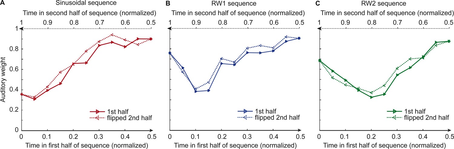
Observers’ relative auditory weights for continuous sequences of visual noise.
Relative auditory weights wA of the 1st (solid) and the flipped 2nd half (dashed) of a period (binned into 20 bins) plotted as a function of the normalized time in the sinusoidal (red), the RW1 (blue), and the RW2 (green) sequences. Relative auditory weights were computed from auditory localization responses of human observers.
Figure 4
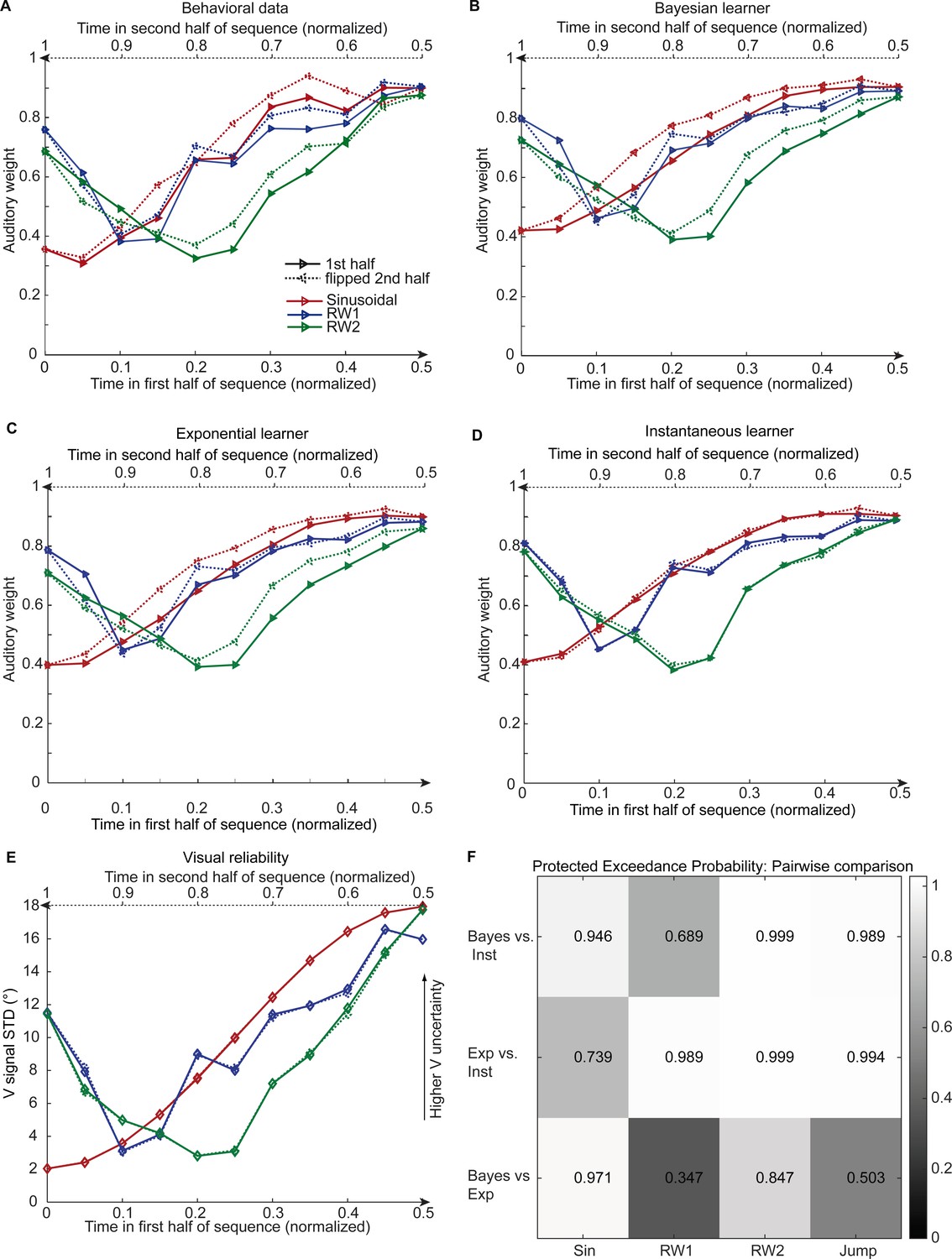
Observed and predicted relative auditory weights for continuous sequences of visual noise.
Relative auditory weights wA of the 1st (solid) and the flipped 2nd half (dashed) of a period (binned into 20 bins) plotted as a function of the normalized time in the sinusoidal (red), the RW1 (blue) and the RW2 (green) sequences. Relative auditory weights were computed from auditory localization responses of human observers (A), Bayesian (B), exponential (C), or instantaneous (D) learning models. For comparison, the standard deviation of the visual signal is shown in (E). Please note that all models were fitted to observers’ auditory localization responses (i.e. not the auditory weight wA). (F) Bayesian model comparison – Random effects analysis: The matrix shows the protected exceedance probability (color coded and indicated by the numbers) for pairwise comparisons of the Instantaneous (Inst), Bayesian (Bayes) and Exponential (Exp) learners separately for each of the four experiments. Across all experiments we observed that the Bayesian or the Exponential learner outperformed the Instantaneous learner (i.e. a protected exceedance probability >0.94) indicating that observers used the past to estimate sensory uncertainty. However, it was not possible to arbitrate reliably between the Exponential and the Bayesian learner across all experiments (protected exceedance probability in bottom row).
Figure 5 with 2 supplements
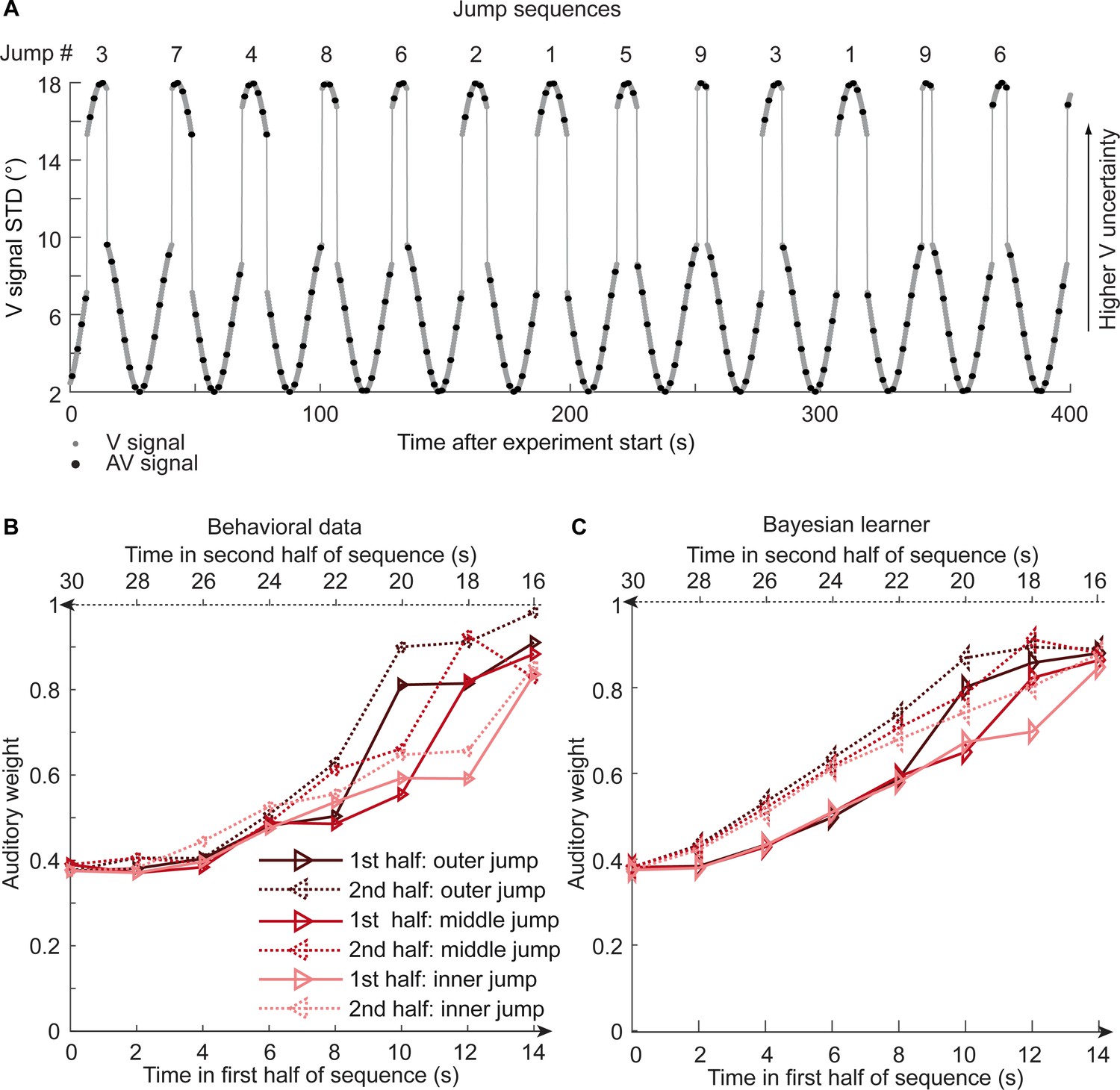
Time course of visual noise and relative auditory weights for sinusoidal sequence with intermittent jumps in visual noise (N = 18).
(A) The visual noise (i.e. STD of the cloud of dots, right ordinate) is displayed as a function of time. Each cycle included one abrupt increase and decrease in visual noise. The sequence of visual clouds was presented every 200 ms (i.e. at 5 Hz) while audiovisual (AV) signals (black dots) were interspersed with an inter-trial asynchrony jittered between 1.4 and 2.8 s. (B, C) Relative auditory weights wA of the 1st (solid) and the flipped 2nd half (dashed) of a period (binned into 15 bins) plotted as a function of the time in the sinusoidal sequence with intermitted inner (light gray), middle (gray), and outer (dark gray) jumps. Relative auditory weights were computed from auditory localization responses of human observers (B) and the Bayesian learning model (C). Please note that all models were fitted to observers’ auditory localization responses (i.e. not the auditory weight wA).
Figure 5—figure supplement 1
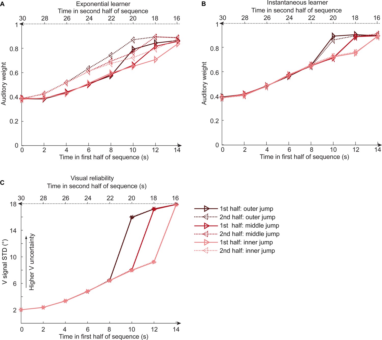
Time course of relative auditory weights and visual noise for the sinusoidal sequence with intermittent jumps in visual noise for the exponential and instantaneous learning models.
Relative auditory weights wA,bin (mean across participants) of the 1st (solid) and the flipped 2nd half (dashed) of a period (binned into 15 time bins) plotted as a function of the time in the sinusoidal sequence with intermitted inner (light gray), middle (gray), and outer (dark gray) jumps. Relative auditory weights were computed from auditory localization responses of exponential (A) or instantaneous (B) learning models. For comparison, the standard deviation of the visual signal is shown in (C). Please note that all models were fitted to observers’ auditory localization responses (i.e. not the auditory weight wA).
Figure 5—figure supplement 2
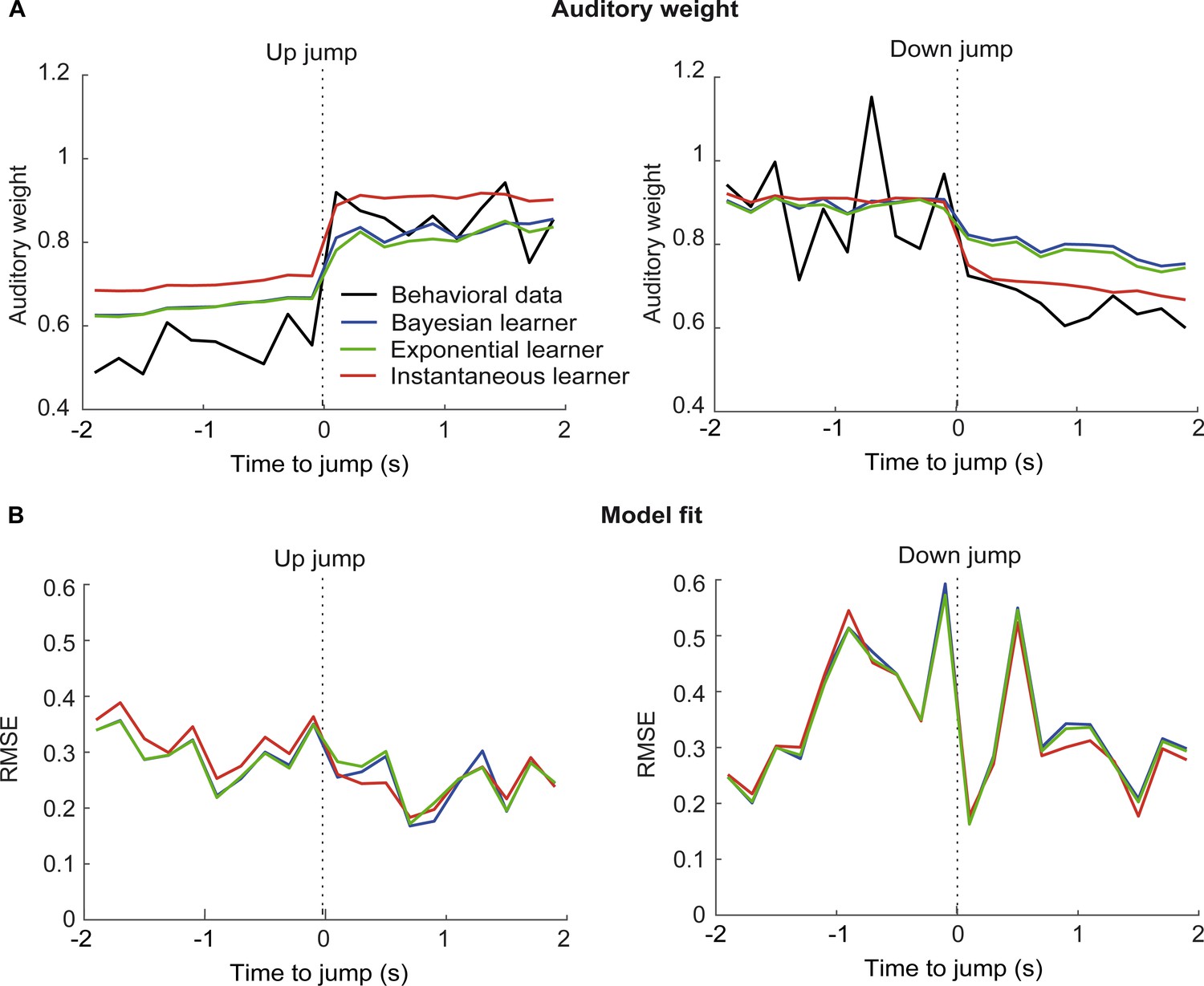
Time course of relative auditory weights and root mean squared error of the computational models before and after the jumps in the sinusoidal sequence with intermittent jumps.
(A) Relative auditory weights wA (mean across participants) shown as a function of time around the up-jumps (left panel) and the down-jumps (right panel) for observers’ behavior, the instantaneous, exponential and Bayesian learner. Relative auditory weights were computed from auditory localization responses for behavioral data and for the predictions of the three computational models in time bins of 200 ms (i.e. 5 Hz rate of the visual clouds). Trials from the three types of up- and down-jumps were pooled to increase the reliability of the wA estimates. Because time bins included only few trials in some participants, individual wA values that were smaller or larger than the three times the scaled median absolute deviation were excluded from the analysis. Note that the up jumps occurred around the steepest increase in visual noise, so that the Bayesian and exponential learners underestimated visual noise (Figure 5C), leading to smaller wA as compared to the instantaneous learner already before the up jump. (B) Root mean squared error (RMSE; computed across participants) between wA computed from behavior and the models’ predictions (as shown in A), shown as a function of the time around the up-jumps (left panel) and the down-jumps (right panel). Please note that all models were fitted to observers’ auditory localization responses (i.e. not the auditory weight wA).
Figure 6
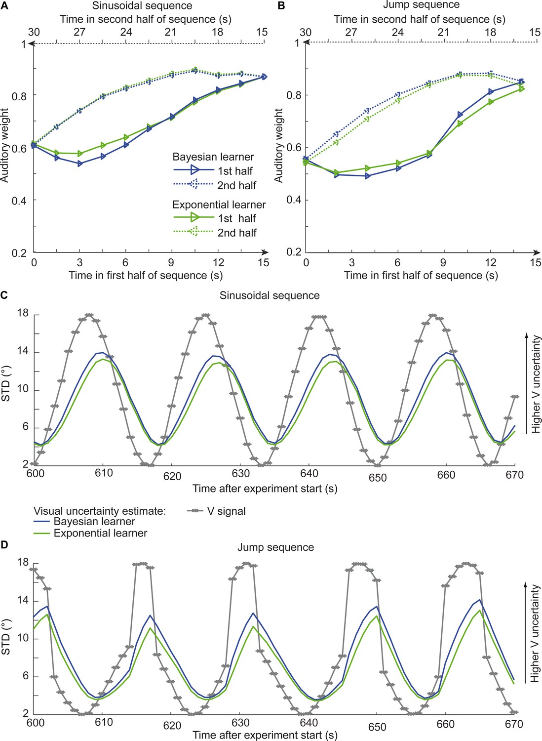
Time course of the relative auditory weights, the standard deviation (STD) of the visual cloud and the STD of the visual uncertainty estimates.
(A) Relative auditory weights wA of the 1st (solid) and the flipped 2nd half (dashed) of a period (binned into 15 bins) plotted as a function of the time in the sinusoidal sequence. Relative auditory weights were computed from the predicted auditory localization responses of the Bayesian (blue) or exponential (green) learning models fitted to the simulated localization responses of a Bayesian learner based on visual clouds of 5 dots. (B) Relative auditory weights wA computed as in (A) for the sinusoidal sequence with intermitted jumps. Only the outer-most jump (dark brown in Figure 5B/C and Figure 5—figure supplement 1) is shown. (C, D) STD of the visual cloud of 5 dots (gray) and the STD of observers’ visual uncertainty as estimated by the Bayesian (blue) and exponential (green) learners (that were fitted to the simulated localization responses of a Bayesian learner) as a function of time for the sinusoidal sequence (C) and in the sinusoidal sequence with intermitted jumps (D). Note that only an exemplary time course from 600 to 670 s after the experiment start is shown.
Appendix 2—figure 1
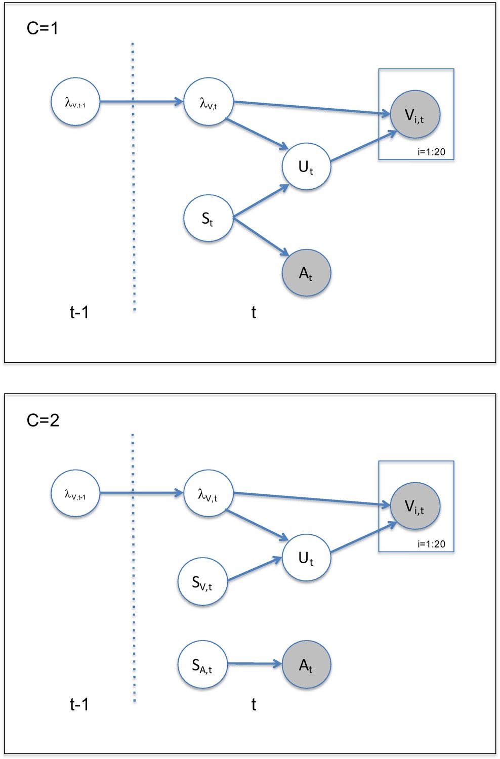
Generative model, for one (C = 1) or two sources (C = 2).
Appendix 2—figure 2
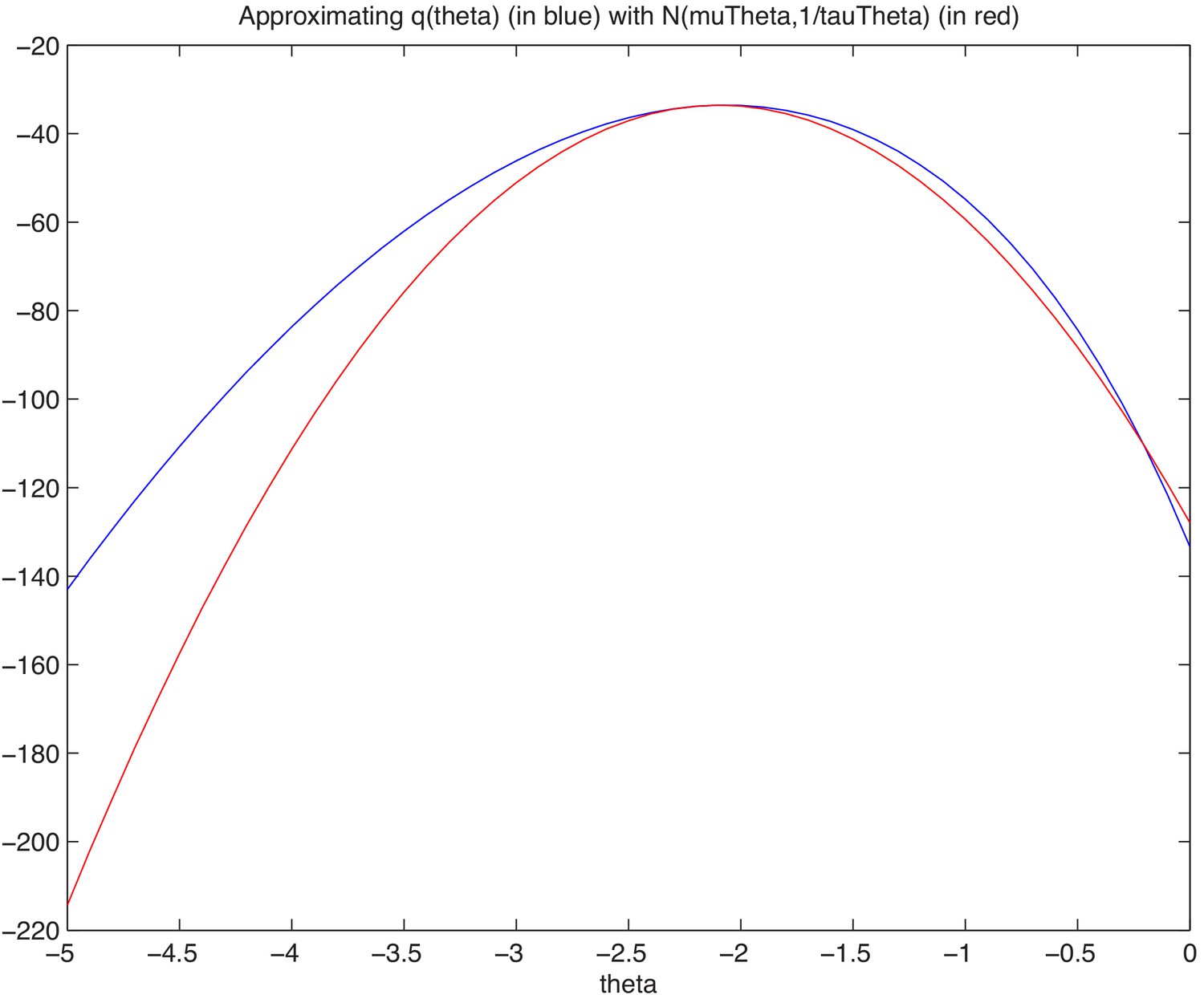
Approximation of theta using Laplace approximation.
Appendix 2—figure 3

Comparing variational Bayes approximation with a numerical discretised grid approximation.
Top row: Example visual stimuli over eight subsequent trials. Middle row: The distribution of estimated sample variance, with no learning over trials. Bottom row: The distribution of _V;t for the Bayesian model that incorporates the learning across trials. Red line is the numerical comparison when using a discretised grid to estimate variance, as opposed to the variational Bayes (green line).
Tables
Table 1
Analyses of the temporal asymmetry of the relative auditory weights across the four sequences of visual noise using repeated measures ANOVAs with the factors sequence part (1st vs. flipped 2nd half), bin and jump position (only for the sinusoidal sequences with intermittent jumps).
| Effect | F | df1 | df2 | p | Partial η2 | |
|---|---|---|---|---|---|---|
| Sinusoid | Part | 12.162 | 1 | 24 | 0.002 | 0.336 |
| Bin | 92.007 | 3.108 | 74.584 | <0.001 | 0.793 | |
| PartXBin | 2.167 | 2.942 | 70.617 | 0.101 | 0.083 | |
| RW1 | Part | 14.129 | 1 | 32 | 0.001 | 0.306 |
| Bin | 76.055 | 4.911 | 157.151 | <0.001 | 0.704 | |
| PartXBin | 1.225 | 4.874 | 155.971 | 0.300 | 0.037 | |
| RW2 | Part | 2.884 | 1 | 18 | 0.107 | 0.138 |
| Bin | 60.142 | 3.304 | 59.467 | <0.001 | 0.770 | |
| PartXBin | 3.385 | 4.603 | 82.849 | 0.010 | 0.158 | |
| Sinusoid with intermittent jumps | Jump | 28.306 | 2 | 34 | <0.001 | 0.625 |
| Part | 24.824 | 1 | 17 | <0.001 | 0.594 | |
| Bin | 76.476 | 1.873 | 31.839 | <0.001 | 0.818 | |
| JumpXPart | 0.300 | 2 | 34 | 0.743 | 0.017 | |
| JumpXBin | 8.383 | 3.309 | 56.247 | <0.001 | 0.330 | |
| PartXBin | 1.641 | 3.248 | 55.222 | 0.187 | 0.088 | |
| JumpXPartXBin | 0.640 | 5.716 | 97.175 | 0.690 | 0.036 |
-
Note: The factor bin comprised nine levels in the first three and seven levels in the fourth sequence. In this sequence, the factor Jump comprised three levels. If Mauchly tests indicated significant deviations from sphericity (p<0.05), we report Greenhouse-Geisser corrected degrees of freedom and p values.
Table 2
Model parameters (median), absolute WAIC and relative.
ΔWAIC values for the three candidate models in the four sequences of visual noise.
| Sequence | Model | σA | Pcommon | σ0 | or γ | WAIC | ΔWAIC |
|---|---|---|---|---|---|---|---|
| Sinusoid | Instantaneous learner | 5.56 | 0.63 | 8.95 | - | 81931.2 | 109.9 |
| Bayesian learner | 5.64 | 0.65 | 9.03 | κ: 7.37 | 81821.3 | 0 | |
| Exponential discounting | 5.62 | 0.64 | 9.02 | γ: 0.23 | 81866.9 | 45.6 | |
| RW1 | Instantaneous learner | 6.30 | 0.69 | 8.46 | - | 110051.2 | 89.0 |
| Bayesian learner | 6.29 | 0.72 | 8.68 | κ: 8.06 | 109962.2 | 0 | |
| Exponential discounting | 6.26 | 0.70 | 8.75 | γ: 0.33 | 109929.9 | −32.3 | |
| RW2 | Instantaneous learner | 6.36 | 0.72 | 10.79 | - | 62576.4 | 201.3 |
| Bayesian learner | 6.49 | 0.78 | 10.9 | κ: 6.7 | 62375.2 | 0 | |
| Exponential discounting | 6.46 | 0.73 | 11.0 | γ: 0.25 | 62421.5 | 46.3 | |
| Sinusoid with intermittent jumps | Instantaneous learner | 6.38 | 0.65 | 8.19 | - | 83891.4 | 94.9 |
| Bayesian learner | 6.45 | 0.68 | 8.26 | κ: 6.13 | 83796.5 | 0 | |
| Exponential discounting | 6.43 | 0.67 | 8.20 | γ: 0.24 | 83798.1 | 1.64 |
-
Note: WAIC values were computed for each participant and summed across participants. A low WAIC indicates a better model. ΔWAIC is relative to the WAIC of the Bayesian learner.
Additional files
-
Supplementary file 1
Seven tables showing results of additional analyses.
- https://cdn.elifesciences.org/articles/54172/elife-54172-supp1-v2.docx
-
Transparent reporting form
- https://cdn.elifesciences.org/articles/54172/elife-54172-transrepform-v2.docx
Download links
A two-part list of links to download the article, or parts of the article, in various formats.
Downloads (link to download the article as PDF)
Open citations (links to open the citations from this article in various online reference manager services)
Cite this article (links to download the citations from this article in formats compatible with various reference manager tools)
Using the past to estimate sensory uncertainty
eLife 9:e54172.
https://doi.org/10.7554/eLife.54172


