Boosts in brain signal variability track liberal shifts in decision bias
- Max Planck UCL Centre for Computational Psychiatry and Ageing Research, Germany
- Center for Lifespan Psychology, Max Planck Institute for Human Development, Germany
- Department of Experimental and Applied Psychology, Vrije Universiteit Amsterdam, Netherlands
- Department of Psychology, University of Amsterdam, Netherlands
Figures
Figure 1 with 1 supplement
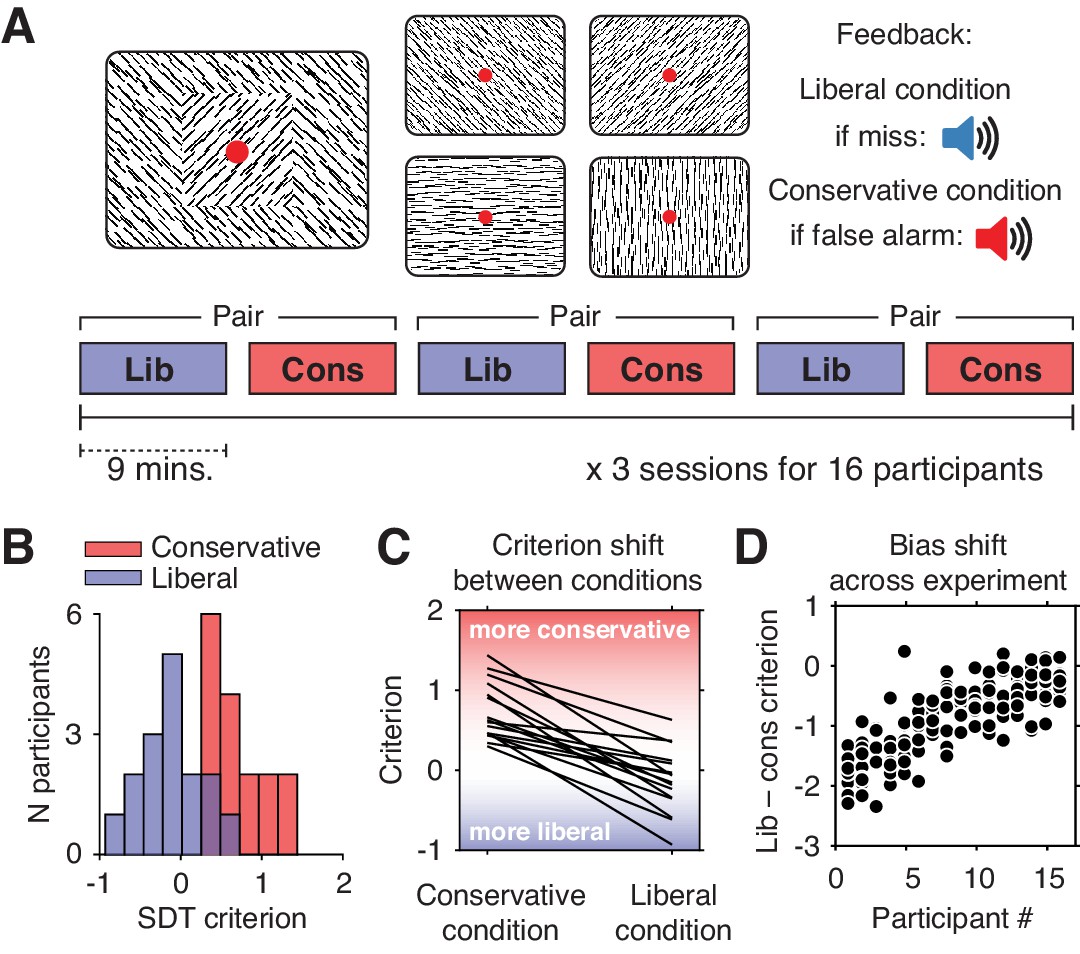
Experimental paradigm and behavioral results.
(A) Top, target and non-target stimuli. Subjects detected targets (left panel) within a continuous stream of diagonal and cardinal line stimuli (middle panel), and reported targets via a button press. In different blocks of trials, subjects were instructed to actively avoid either target misses (liberal condition) or false alarms (conservative condition). Auditory feedback was played directly after the respective error in both conditions (right panel). Bottom, time course of an experimental session. The two conditions were alternatingly administered in blocks of nine minutes. In between blocks participants were informed about current task performance and received instructions for the next block. Subsequent liberal and conservative blocks were paired for within-participant analyses (see panel D, and Figure 3C). (B) Distributions of participants’ criterion in both conditions. A positive criterion indicates a more conservative bias, whereas a negative criterion indicates a more liberal bias. (C) Lines indicating the criteria used by each participant in the two conditions, highlighting individual differences both in overall criterion (line intercepts), and in the size of the criterion shift between conditions (slopes). (D) Within-person bias shifts for liberal–conservative block pairs (see panel A, bottom). Participants were sorted based on average criterion shift before plotting.
Figure 1—figure supplement 1
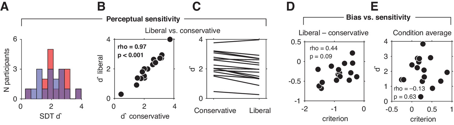
Perceptual sensitivity and relationship between decision bias and sensitivity.
(A) Distributions of participants’ d' in both conditions. A higher d' indicates higher sensitivity. (B) Scatter plot depicting the correlation between participant’s d' in both conditions. (C) Corresponding individual participant slopes. (D) Correlation between d' and criterion averaged across conditions. (E) Correlation between liberal – conservative d' and liberal – conservative criterion.
Figure 2
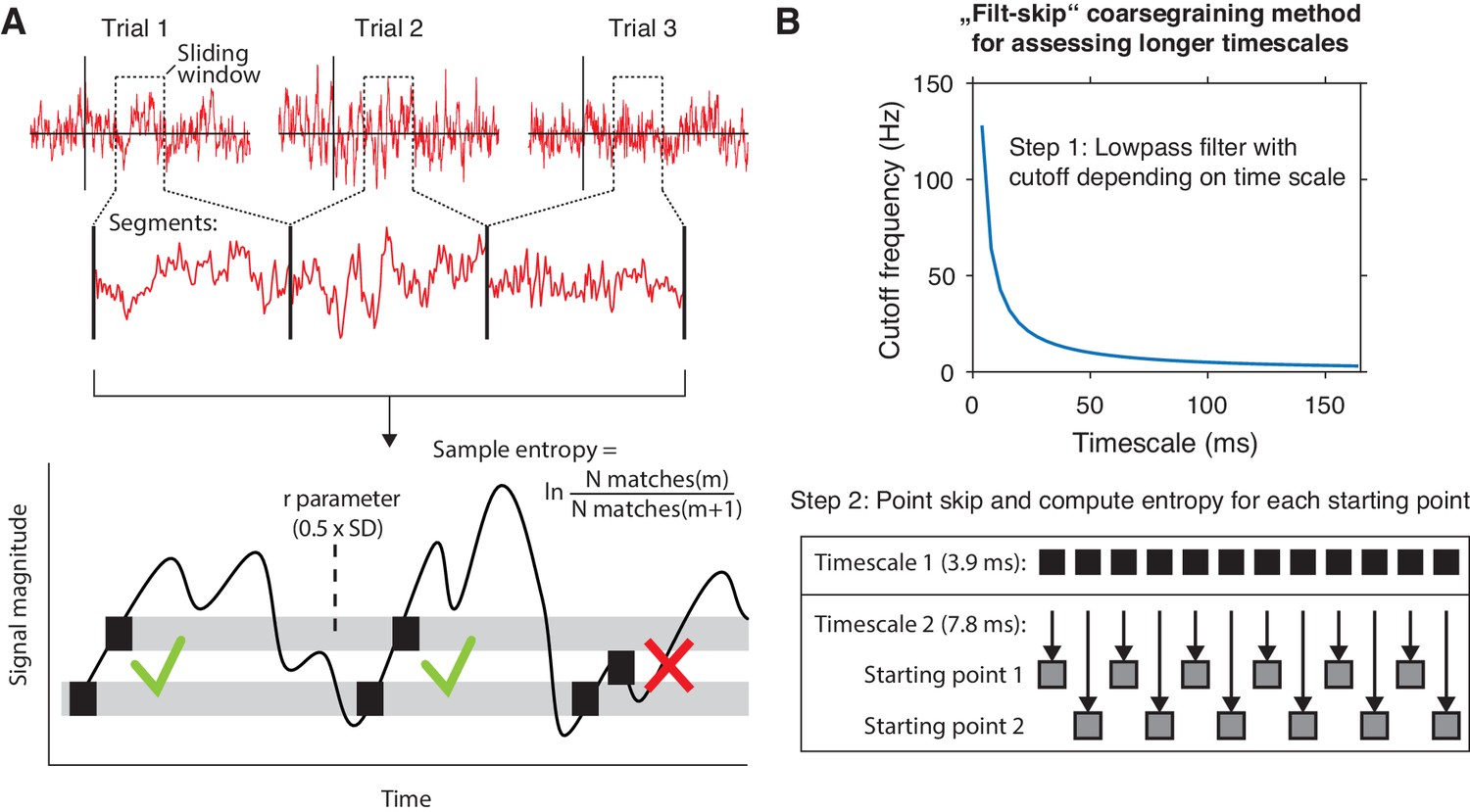
mMSE estimation procedure.
(A) Discontinuous entropy computation procedure. Data segments of 0.5 s duration centered on a specific time point from each trial’s onset (top row) are selected and concatenated (middle row). Entropy is then computed on this concatenated time series while excluding discontinuous segment borders by counting repeats of both m (here, m = 1 for illustration purposes) and m+1 (thus 2) sample patterns and taking the log ratio of the two pattern counts (bottom row). We used m = 2 in our actual analyses. The pattern similarity parameter r determines how lenient the algorithm is toward counting a pattern as a repeat by taking a proportion of the signal’s standard deviation (SD), indicated by the width of the horizontal gray bars. The pattern counting procedure is repeated at each step of the sliding window, resulting in a time course of entropy estimates computed across trials. (B) ‘Filt-skip’ coarsegraining procedure used to estimate entropy on longer timescales, consisting of low-pass filtering followed by point-skipping. Filter cutoff frequency is determined by dividing the data sampling rate (here, 256 Hz i.e. 1 sample per 3.9 ms) by the index of the timescale of interest (top row). The signal is then coarsened by intermittently skipping samples (bottom row). In this example, every second sample is skipped at timescale 2, resulting in two different time courses depending on the starting point. Patterns are counted independently for both starting points and summed before computing entropy.
Figure 3 with 5 supplements
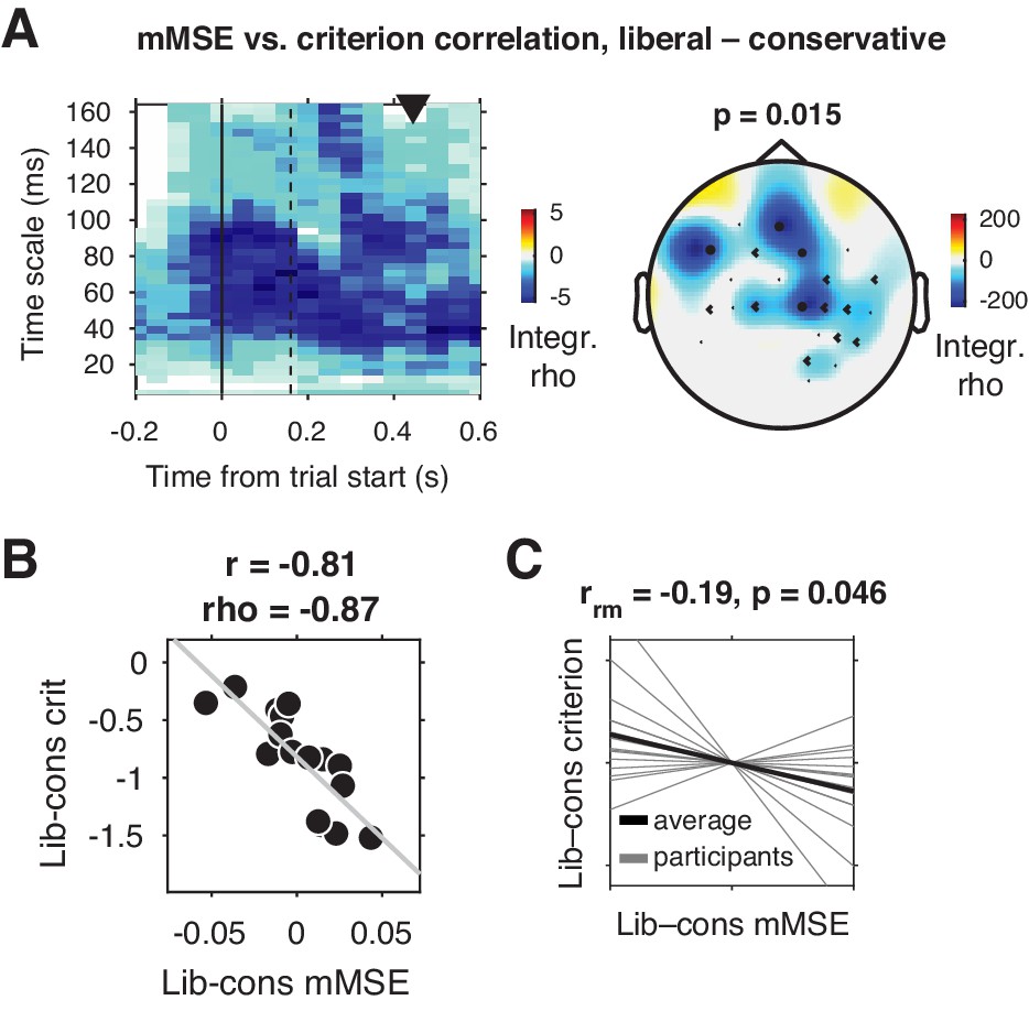
Change-change correlation between liberal–conservative shifts in mMSE and bias.
(A) Significant negative electrode-time-timescale cluster observed via Spearman correlation between liberal–conservative mMSE and liberal–conservative SDT criterion, identified using a cluster-based permutation test across participants to control for multiple comparisons. Correlations outside the significant cluster are masked out. Left panel, time-timescale representation showing the correlation cluster integrated over the electrodes included in the cluster, indicated by the black dots in the topographical scalp map in the right panel. Dot size indicates how many time-timescale bins contribute to the cluster at each electrode. Color borders are imprecise due to interpolation used while plotting. The solid vertical line indicates the time of trial onset. The dotted vertical line indicates time of (non)target onset. Right panel, scalp map of mMSE integrated across time-timescale bins belonging to the cluster. p-Value above scalp map indicates statistical significance of the cluster. The black triangle indicates participants’ median reaction time, averaged across participants and conditions. (B) Scatter plot of the correlation after averaging mMSE within time-timescale-electrode bins that are part of the three-dimensional cluster. Since the cluster was defined based on significant change-change correlations, averaging mMSE across the significant time-timescale-electrode bins before correlating represents no new information. Thus, the scatter plot serves only to illustrate the negative relationship identified in panel A. Both Pearson’s r and Spearman’s rho are indicated. We report no p-values since the bin selection procedure guarantees significance, and consider the correlation a descriptive statistic only. (C) Within-participant mMSE vs. criterion slopes across liberal–conservative block pairs completed across the experiment. rrm, repeated measures correlation across all block pairs performed after centering each participant’s shifts in mMSE and criterion around zero by removing the intercept. Gray lines, individual participant slopes fit across liberal–conservative mMSE vs criterion block pairs. Black line, slope averaged across participants.
-
Figure 3—source data 1
This MATLAB file contains the data for Figure 3A and B.
- https://cdn.elifesciences.org/articles/54201/elife-54201-fig3-data1-v1.mat.zip
-
Figure 3—source data 2
This csv file contains the data for Figure 3C.
- https://cdn.elifesciences.org/articles/54201/elife-54201-fig3-data2-v1.csv
Figure 3—figure supplement 1
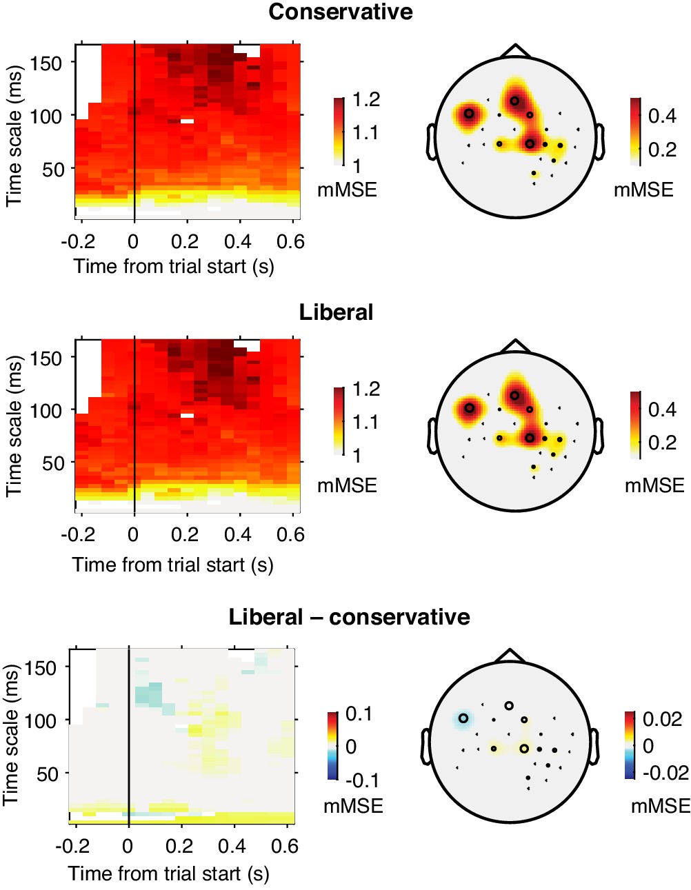
Raw mMSE values averaged across subjects within the correlation cluster identified in Figure 3A.
Raw mMSE values were averaged within the electrode-time-timescale cluster identified in the change-change correlation analysis with criterion. The bottom panel shows the Liberal–conservative contrast with small range on the color scale, indicating the lack of a main effect of condition in our data.
Figure 3—figure supplement 2
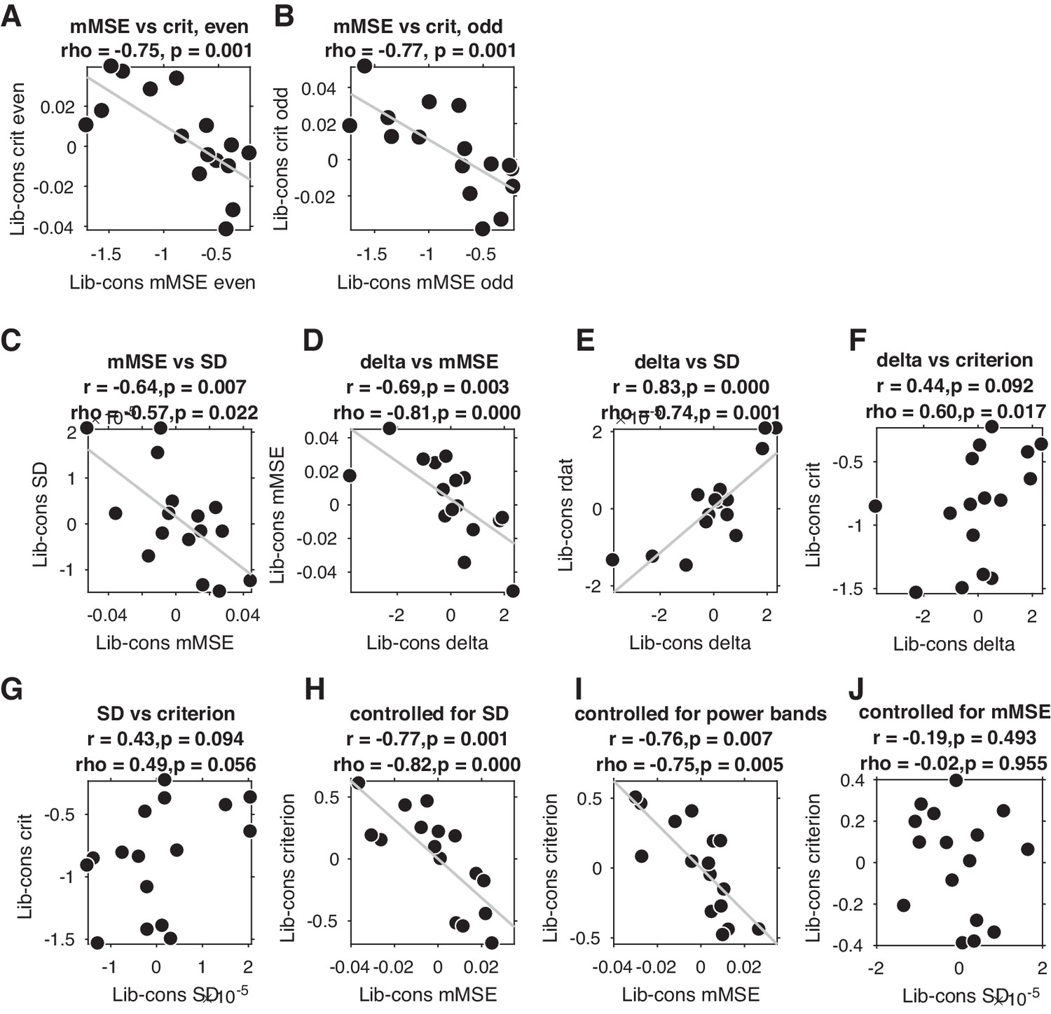
Correlations between liberal–conservative shifts in mMSE versus criterion in split data, and versus EEG signal SD and spectral power.
(A.B) Across-participant change-change correlations in both data halves after arbitrary split into even trials (A) and odd trials (B). (C – J) Scatter plots of various change-change correlations. See titles and axes labels of each plot for details. Least squares lines (gray) were plotted when the Pearson correlation reached significance (p<0.05). Both the signal SD (panel C) and delta (panel D) were negatively correlated with mMSE, whereas the other canonical frequency bands correlated only weakly (theta, rho = –0.31; alpha, rho = 0.18; beta, rho = 0.26; gamma, rho = 0.29, all p>0.24). Signal SD and delta were also correlated with each other (rho = 0.74, p=0.001, panel E), indicating that delta contributed strongly to overall signal SD, as expected based on the known 1/f characteristic of neural data. Neither liberal–conservative delta (panel F) nor SD (panel G) correlated as strongly with the criterion shift as liberal–conservative mMSE (see Figure 3B). In contrast, the correlation between SD and criterion was not significant when controlling for mMSE (panel J), highlighting the unique ability of mMSE to explain the bias shift.
Figure 3—figure supplement 3
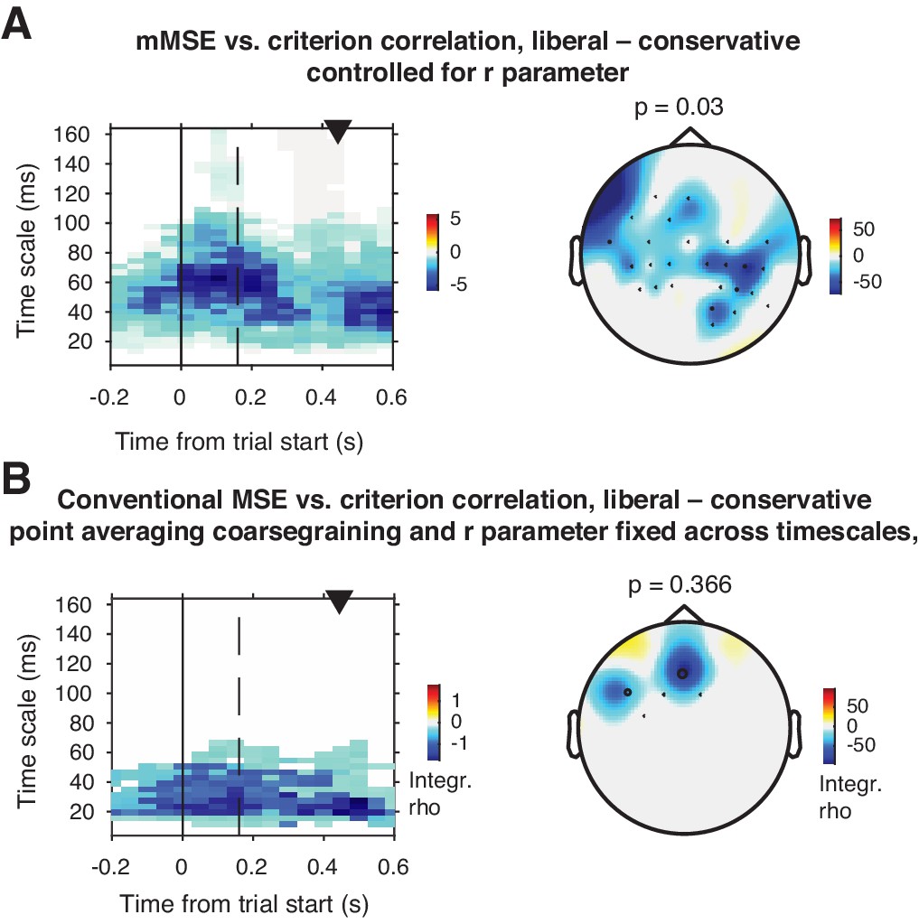
Control analyses investigating signal SD and point averaging method.
(A) Liberal – conservative mMSE vs. criterion correlation when statistically controlling for the r parameter (signal SD) across participants. The cluster remains significant and the topography is similar, but the effect is more widespread across electrodes, and less widespread across timescales. (B) As A. but using traditional MSE, including coarse graining through point averaging to asses longer timescales and a fixed r parameter across timescales. The cluster does not reach significance.
Figure 3—figure supplement 4
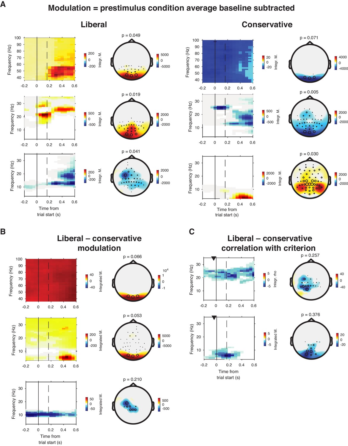
EEG spectral power normalized by subtracting the condition-average pre-trial baseline.
In addition to the condition-specific baseline used in our previous paper (Kloosterman et al., 2019), we also computed spectral power modulation using a condition-averaged baseline correction based to investigate the link between spectral power and our experimental manipulation. Power modulation were similar to those reported in our previous paper. (A) Significant clusters found within the liberal (left panels) and conservative (right panels) conditions. (B) Liberal – conservative contrast, showing stronger broadband power modulation in the liberal condition, except in the alpha range. Please see our previous paper for detailed analysis of the alpha effect. (C) Change-change correlations between liberal–conservative shifts in power modulation and decision bias. We observed two clusters (rows), none of which were significant after multiple comparison correction.
Figure 3—figure supplement 5
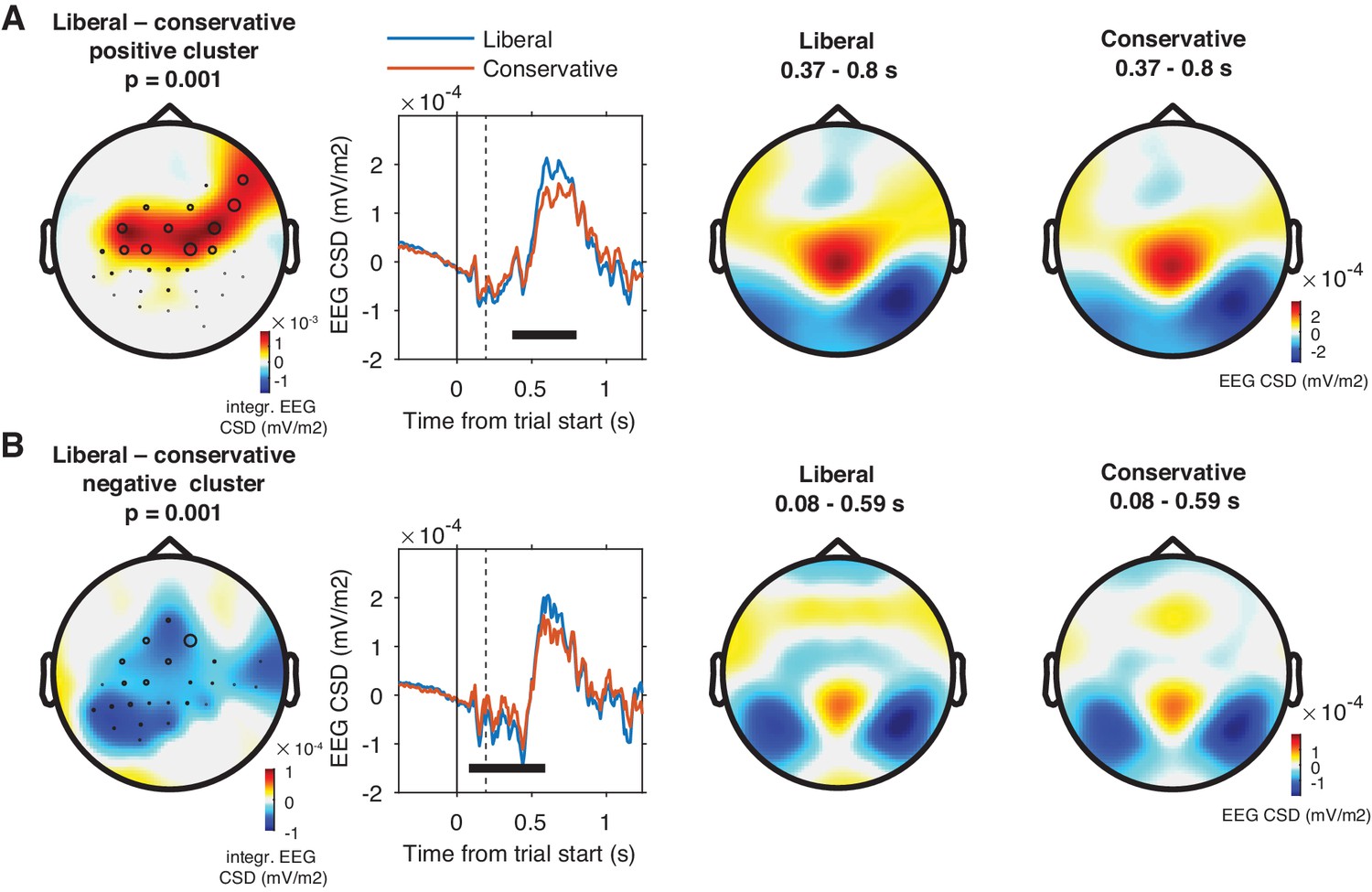
Event-related responses in both conditions.
(A) Positive (liberal >conservative) cluster in parietal and central electrodes between 0.37 and 0.8 s after trial onset. (B) Negative (conservative >liberal) cluster in parietal and central electrodes between 0.08 and 0.59 s after trial onset. Conventions as in Figure 3.
Figure 4
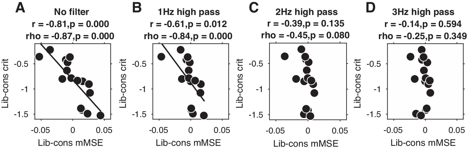
Liberal–conservative change-change correlation between mMSE and decision bias for non-filtered data (A) and after 1,2, and 3 Hz high-pass filtering (B C and D).
Figure 5
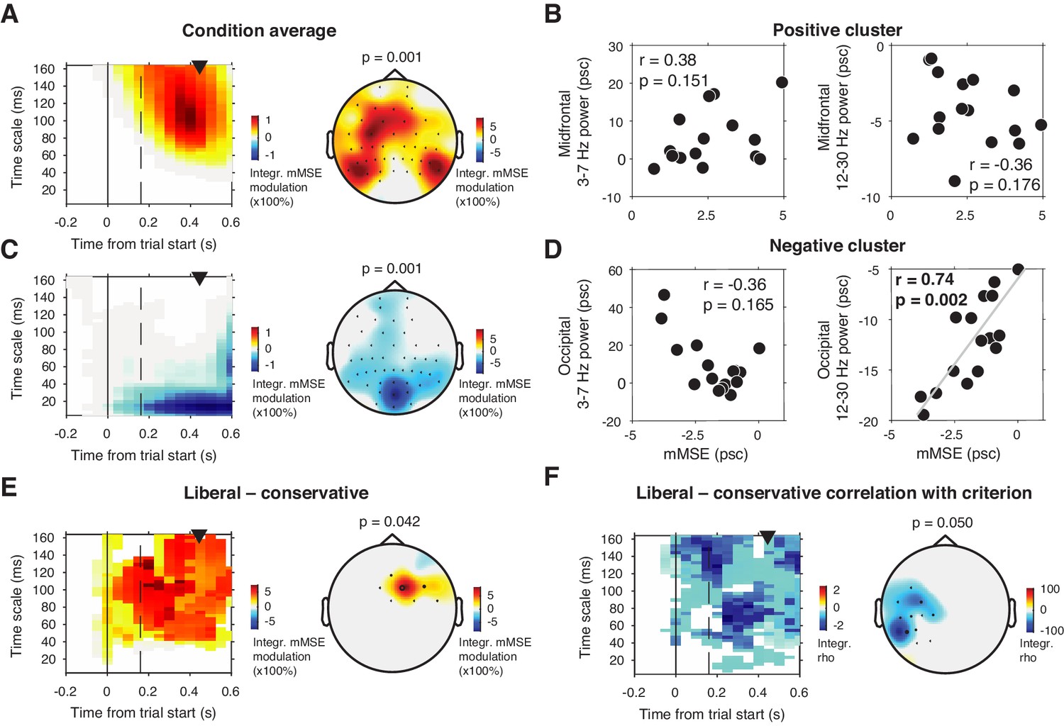
mMSE modulation with respect to pre-trial baseline.
(A) Significant positive cluster observed in longer timescales after normalizing mMSE values to percent signal change (psc) units with respect to the pre-trial baseline (–0.2 to 0 s) and averaging across conditions. (B) Correlation between mMSE modulation in the positive cluster depicted in A and spectral power modulation in midfrontal electrodes. Left panel, 3–7 Hz; right panel, 12–30 Hz. (C and D) As B but for the posterior negative cluster. (E) Significant positive cluster observed in mid-frontal electrodes in the liberal–conservative contrast of mMSE modulation. (F) Significant cluster resulting from the correlation between liberal–conservative mMSE modulation with liberal–conservative SDT criterion. Conventions as in Figure 3.
Tables
Key resources table
| Reagent type (species) or resource | Designation | Source or reference | Identifiers | Additional information |
|---|---|---|---|---|
| Biological sample (Humans) | Participants | Kloosterman et al., 2019 | https://doi.org/10.7554/elife.37321 | See Subjects section in Materials and methods |
| Software, algorithm | MATLAB | Mathworks | MATLAB_R2016b, RRID:SCR_001622 | |
| Software, algorithm | Presentation | NeuroBS | Presentation_v9.9, RRID:SCR_002521 | |
| Software, algorithm | Statistical Analysis | R | R version 4.0.1, RRID:SCR_001905 | |
| Software, algorithm | Custom analysis code | Kloosterman et al., 2019 | https://github.com/kloosterman/critEEG | |
| Software, algorithm | Custom analysis code | Kloosterman et al., 2019 | https://github.com/kloosterman/critEEGentropy | |
| Software, algorithm | Custom analysis code | Kloosterman, 2020 | https://github.com/LNDG/mMSE/ | FieldTrip-compatible toolbox |
| Other | EEG data experimental task | Kloosterman et al., 2019 | https://doi.org/10.6084/m9.figshare.6142940 |
Additional files
Download links
A two-part list of links to download the article, or parts of the article, in various formats.
Downloads (link to download the article as PDF)
Open citations (links to open the citations from this article in various online reference manager services)
Cite this article (links to download the citations from this article in formats compatible with various reference manager tools)
Boosts in brain signal variability track liberal shifts in decision bias
eLife 9:e54201.
https://doi.org/10.7554/eLife.54201


