Stable and dynamic representations of value in the prefrontal cortex
- Nash Family Neuroscience Department, Icahn School of Medicine at Mount Sinai, United States
- Friedman Brain Institute, Icahn School of Medicine at Mount Sinai, United States
- Helen Wills Neuroscience Institute, University of California at Berkeley, United States
- Department of Psychology, University of California at Berkeley, United States
Figures
Figure 1
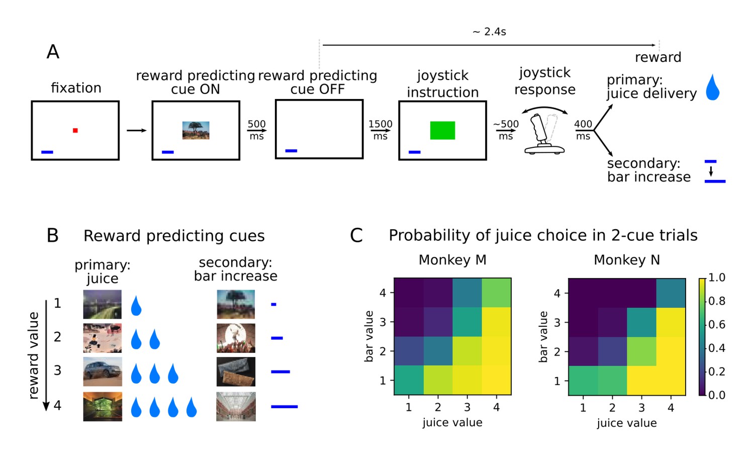
Value-based decision making task.
(A) Monkeys initiated a trial by fixating a point in the center of the screen. A reward predicting cue appeared that the subject was required to fixate for 450 ms. After a 1500 ms delay, one of two possible images instructed the monkey to move a joystick right or left. Contingent on a correct joystick response, monkeys received a reward either in the form of juice (primary) or an increase of a reward bar (secondary), which was constantly displayed on screen (blue bar in figure). Note that the presentation of the reward predicting cue and the delivery of the reward are separated in time by more than 2 s. (B) A total of eight reward predicting pictures covered the combinations of four possible values, and two reward types. (C) Probability of choosing a juice option in choice trials for every pair of cues in which one predicts a juice reward and the other a bar reward.
Figure 2 with 2 supplements
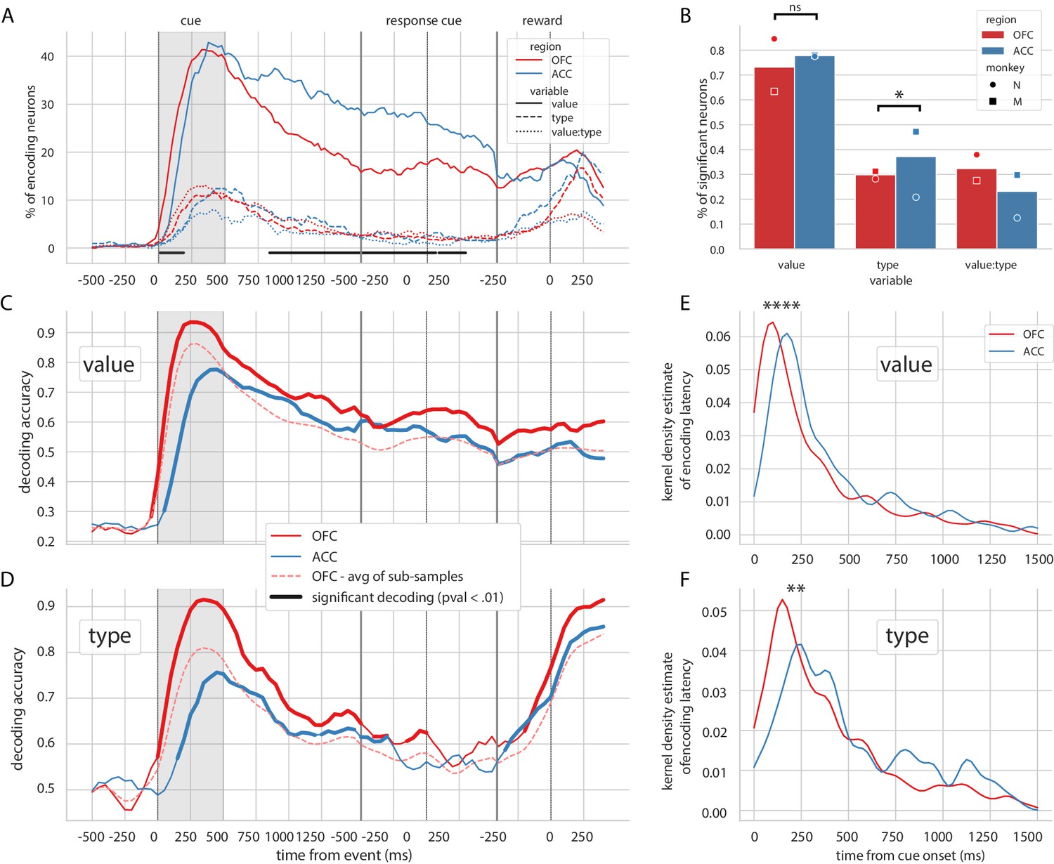
Encoding and decoding of task variables.
(A) Percentage of units encoding the different variables at each point in time in both OFC and ACC. Significant difference in value encoding neurons with χ2 test is indicated by thick black lines at the bottom (p≤0.01). (B) Percentage of units encoding the task variables at any point in time from the onset of cue presentation to the delivery of the reward. (C and D) Average decoding accuracy of value and type, respectively, across five randomly generated population data sets, with a ridge regression classifier. Significant decoding is shown by the thick portions of line and corresponds to the time bins where the aggregated p-value of 1000-permutation tests for each of the five data sets was lower than 0.01. The dashed red line is the average of 200 sub-samples of OFC data with the same number of units as in ACC for comparison. (E and F) Kernel density estimate of encoding latencies in units for value and type, respectively. OFC latencies are significantly shorter (see main text).
Figure 2—figure supplement 1
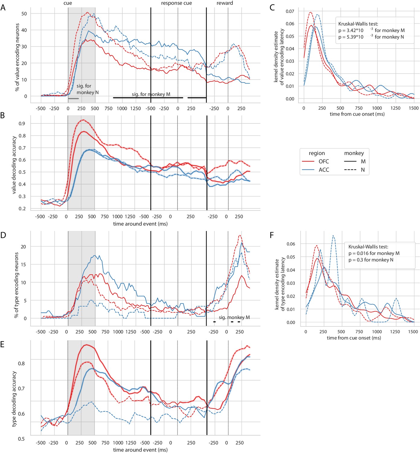
Encoding and decoding of value and type for each monkey.
In each plot, OFC and ACC are represented with red and blue respectively, and monkey M and N with plain and dashed lines. (A) Percentage of units encoding value at each point in time. Significant difference in value encoding neurons with χ2 test is indicated by thick black/grey lines at the bottom (p≤0.01) for monkey M/N. (B) Average value decoding accuracy across five randomly generated population data sets, with a ridge regression classifier. Significant decoding is shown by the thick portions of line and corresponds to the time bins where the aggregated p-value of 1000-permutation tests for each of the five data sets was lower than 0.01. (C) Kernel density estimate of unit value encoding latencies. D, E and F correspond to A, B and C for variable type.
Figure 2—figure supplement 2

Example neurons with nonlinear encoding of value.
Average firing rate of six example neurons showing a non-linear relationship with value. Green and black curves represent averaged z-scored firing rate for juice and bar trials, respectively. Error bars represent the standard error of the mean. These example neurons are significant for value with an ANOVA, not significant for the interaction of value and type with the same ANOVA and not significant for value in a linear regression.
Figure 3 with 2 supplements
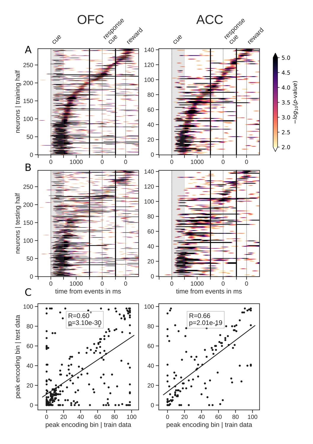
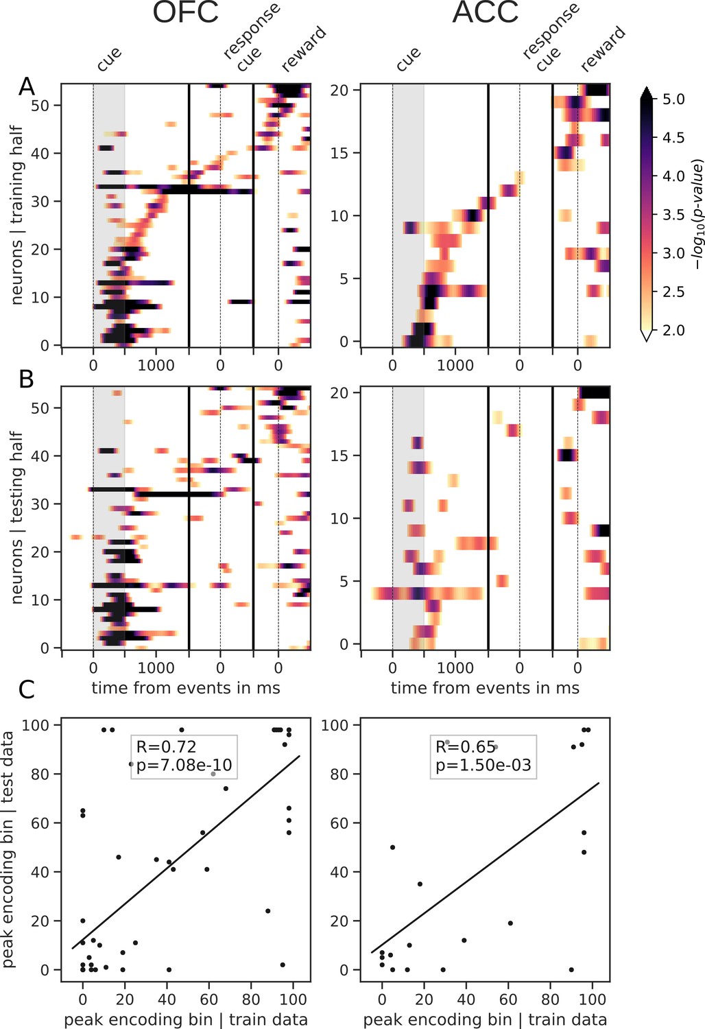
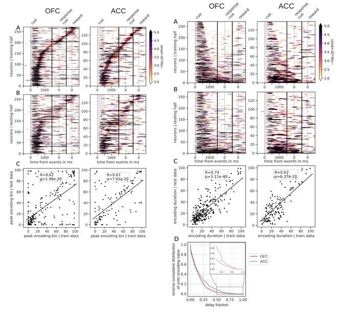
Tiling of the delay by value encoding units.
(A) Tiling of individual units according to their peak encoding of value across the delay in both OFC and ACC with the training half of the trials. Colors represent the negative log of the encoding p-value (ANOVA, F test on value). The measure is bounded between 2 and 5 for visualization and corresponds to p-values ranging from 0.01 to 10−5. (B) Tiling with the testing half of the trials, with units sorted according to the training half of the trials, to show consistency in sequential encoding. Note that only units that had significant encoding in both the training and testing dataset were included, hence the lower number of units. (C) Scatter plot of the peak encoding bin for training versus testing half of the data. Graphs show the Spearman correlation coefficient, R, with associated p-value, p, and trendline.
Figure 3—figure supplement 1
Tiling and spanning of delay with unit firing rate.
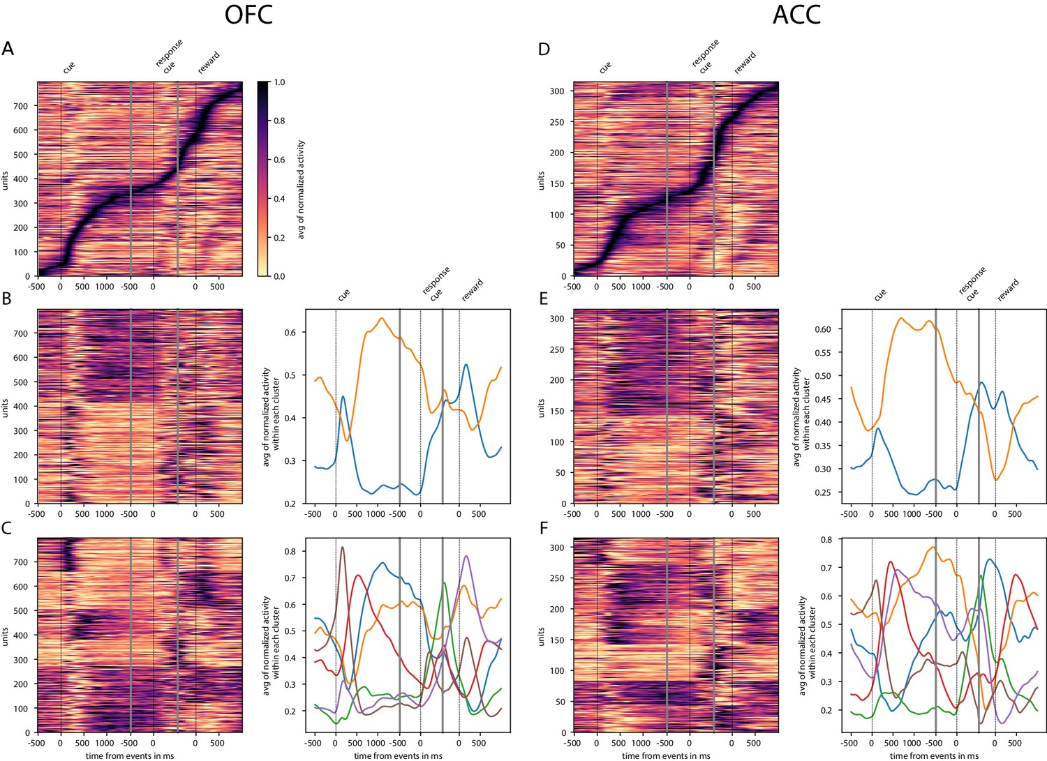
Activity of neurons was averaged across trials and normalized so that activity is scaled between 0 and 1. (A) Tiling of the delay by OFC activity and surrounding epochs. (B) Clustering of OFC activity in two clusters with K-means clustering. Left graph shows the activity of each unit sorted by cluster. In the right graph, each curve is the averaged activity across all the units within a cluster. (C) Same as B with six clusters (determined with elbow method) instead of 2. D, E and F are identical to A, B and C with ACC data instead of OFC. Events occurring at times indicated by 0 on the x-axis are: reward cue on, joystick instruction cue on, and reward delivery.
Figure 3—figure supplement 2
Tiling of the delay by reward type encoding units.
Same as main figure for reward type. Panels A, B and C correspond to the panels A, B and C in the main figure but for reward type instead of reward value.
Figure 4 with 1 supplement
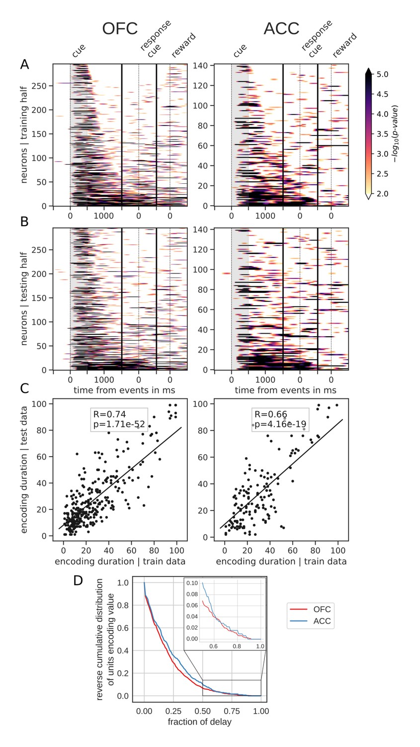
Spanning of the delay by value encoding units.
(A) Units sorted by the duration of encoding of value with the training half of the trials. Colors represent the negative log of the encoding p-value (ANOVA, F test on value). The measure is bounded between 2 and 5 for visualization and corresponds to p-values ranging from 0.01 to 10−5. (B) Encoding durations of the testing half of the trials sorted by the duration the training trials. (C) Scatter plot of encoding duration for training versus testing half of the data. Graphs show the Spearman correlation coefficient, R, with associated p-value, p, and trendline. (D) Reverse cumulative distribution of units encoding value as a function of the fraction of the delay covered. This graph shows the proportion of units encoding value for at least the fraction of the delay indicated on the x-axis (no significant difference between regions, see main text).
Figure 4—figure supplement 1

Spanning of the delay by reward type encoding units.
Same as main figure for reward type. Panels A, B, C and D correspond to the panels A, B, C and D in the main figure but for reward type instead of reward value.
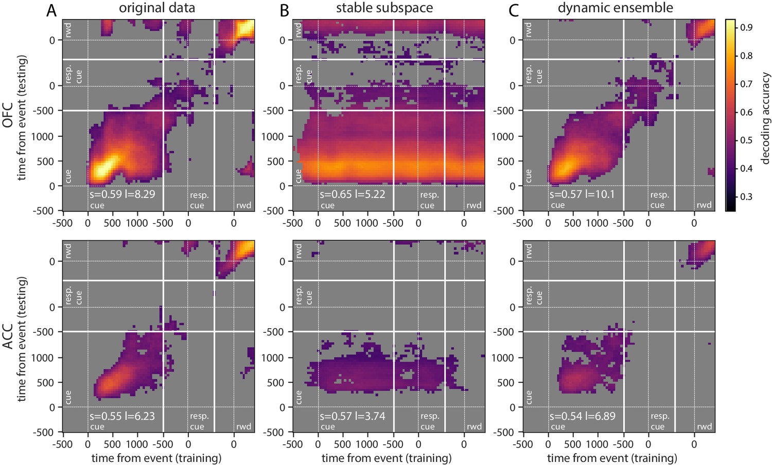
Figure 5 with 3 supplements
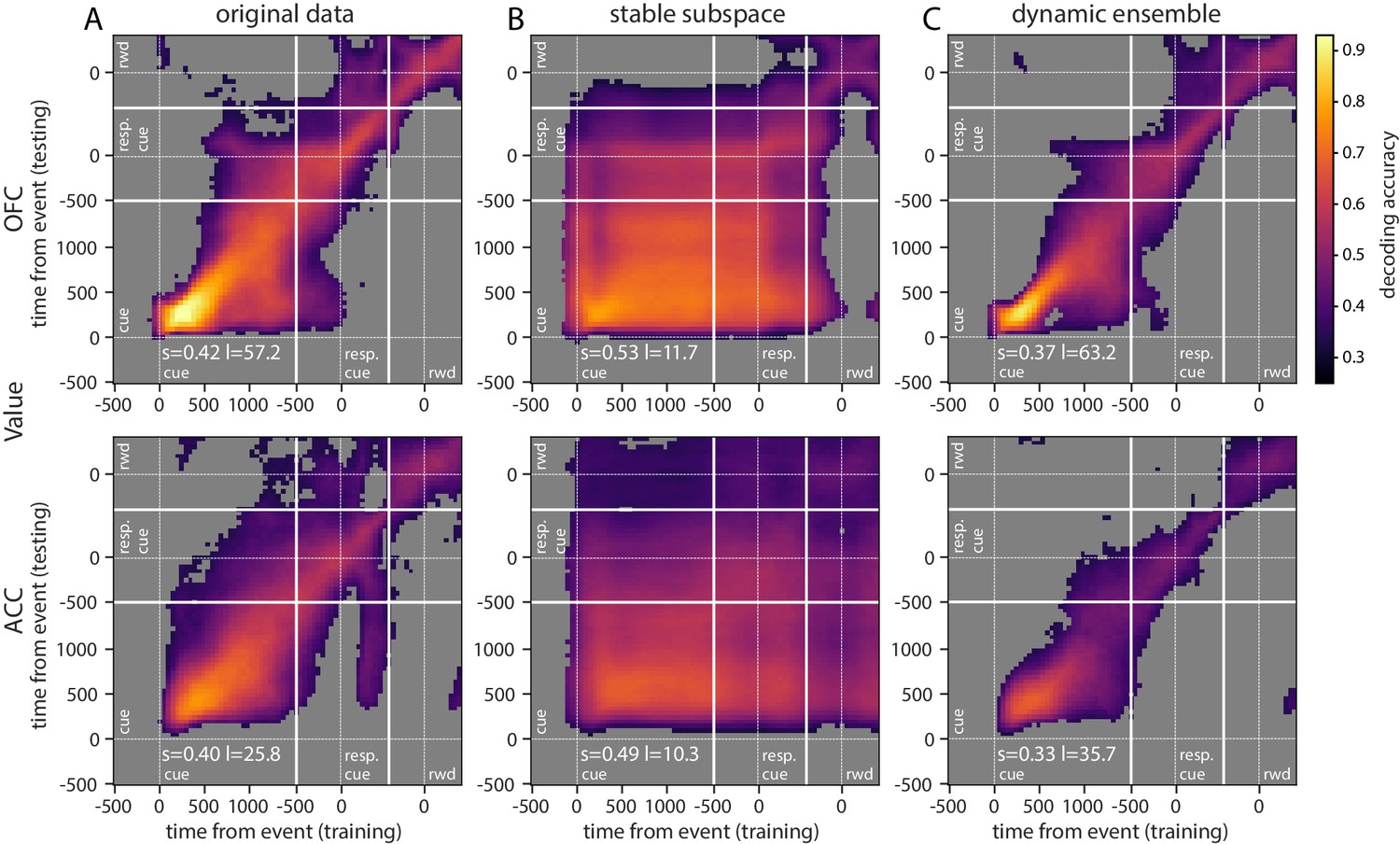
Accuracy of cross-temporal decoding (CTD) of value with different methods.
Training and testing of a ridge classifier at different time bins across the delay. CTD was applied to (A) original data, (B) a stable subspace obtained from the combination of a value subspace and an ensemble method where units are iteratively removed to obtain maximum accuracy, and (C) on a dynamic ensemble where units were iteratively removed from the ensemble to maximize a dynamic score. Thick white lines indicate junctions between the three successive epochs (cue presentation, joystick task and reward delivery). The thin dashed white lines indicate the reference event of each epoch (reward predicting cue onset, response instruction, reward). The decoding accuracy corresponds to the average of five randomly generated pseudo populations and non-significant accuracy has been greyed out for clarity. The p-value threshold is 0.01 and p-values were obtained by aggregating the p-values of each dataset for a given training/testing time bin pair (see Methods section for more details; rwd = reward, resp. cue = response cue). The stable and locality scores are displayed on each panel (s = stability score, l = locality score). Note that significant decoding before the presentation of the cue is due to smoothing.
Figure 5—figure supplement 1
Cross-temporal decoding of reward type.
Accuracy of cross-temporal decoding (CTD) of type with different methods. Same as main figure for reward type.
Figure 5—figure supplement 2
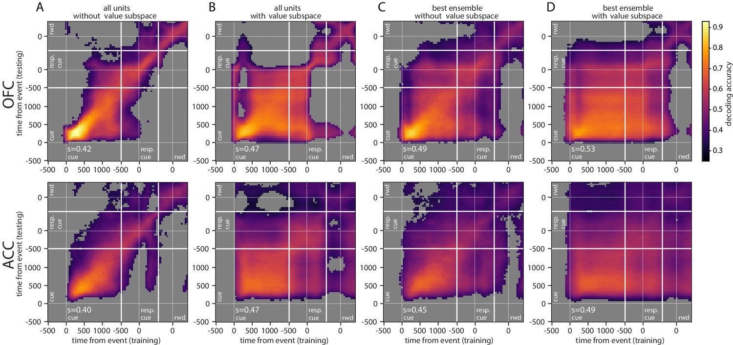
Cross-temporal decoding of value with ensemble and subspace methods independently.
Cross-temporal decoding without (A, C) or with (B, D) a value subspace, and with the full population (A, B) or with the best ensemble (C, D). Thick white lines indicate junctions between the three successive epochs (cue presentation, joystick task and reward delivery). The thin dashed white lines indicate the reference event of each epoch (reward predicting cue onset, response instruction, reward). The contour curve indicates areas with a p-value lower than 0.01 with a 2000 fold permutation test. (rwd = reward, resp. cue = response cue, s = stability score).
Figure 5—figure supplement 3
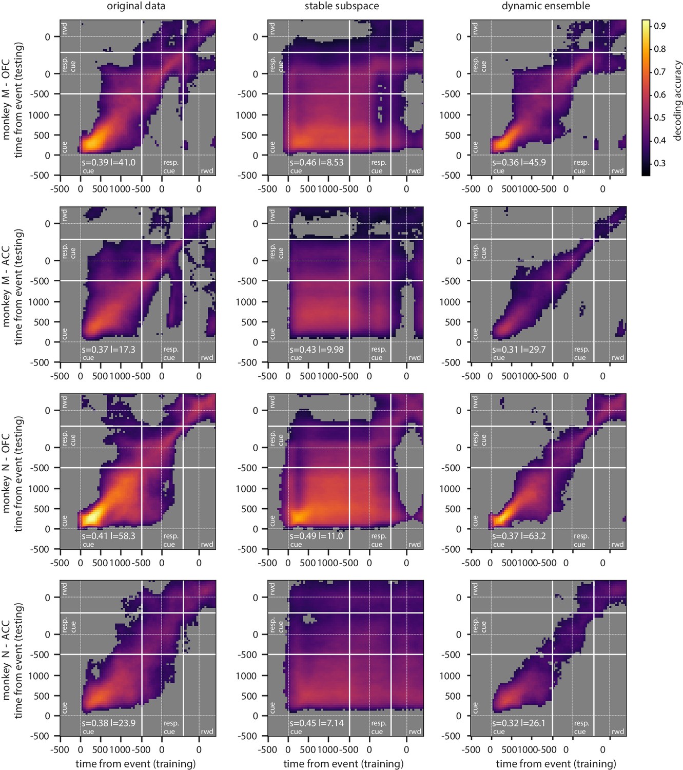
Cross-temporal decoding of value for each monkey independently.
Cross-temporal decoding accuracy of value with different methods for each monkey. Each row correspond to a different combination of monkey and region, as indicated at the left of each row. Since results are similar across rows, they are largely independent of monkey and region.
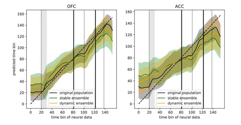
Figure 6
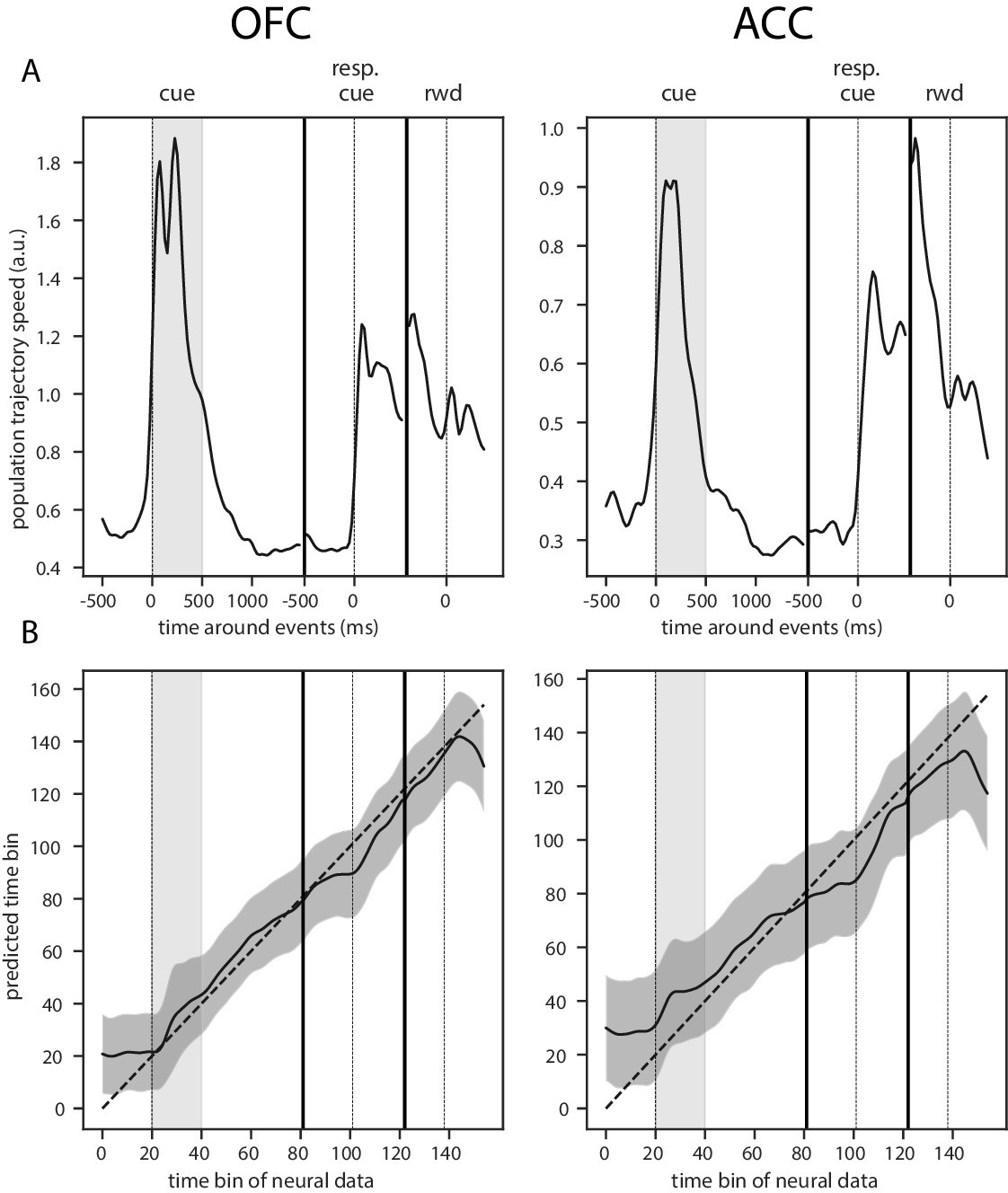
Trajectory speed and regression of time.
(A) Speed (rate of change) of the average activity trajectory in the neural space defined by the full population of neurons, in OFC (left) and ACC (right). Note that the difference in scale between OFC and ACC (y-axis) is due to the difference in the number of units in each population. (B) Regression of the time bin from population activity with a simple linear regression. The black line and shaded area represent the average and standard deviation of leave-one-out cross-validation results. The dashed line corresponds to ground truth. For more temporally accurate results, the firing rate of each unit was estimated with a 50 ms standard deviation Gaussian kernel instead of the 100 ms used in the other analyses.
Figure 7
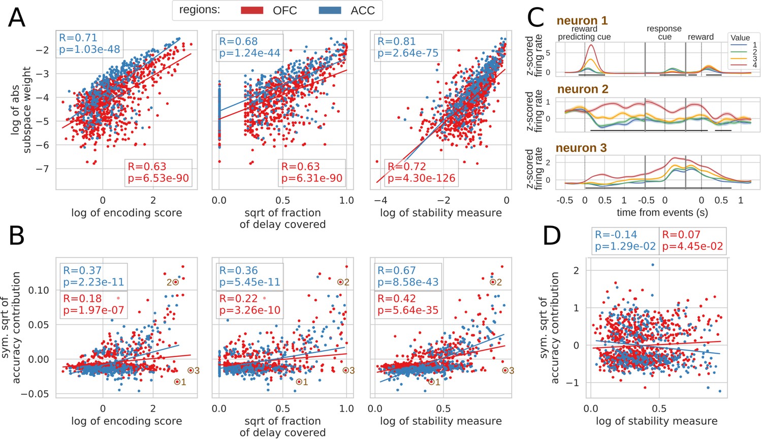
Correlation between encoding and decoding measures.
(A) Correlations between encoding measures and subspace weights. (B) Correlations between encoding measures and CTD accuracy contribution. (C) Z-scored firing rate of two example neurons negatively contributing to the stable ensemble (1 and 3) and one neuron contributing positively (2). Individual data points corresponding to these neurons are circled in B. (D) Correlations between stability measure and locality measure contribution. All figures show Spearman correlations. sqrt = square root; negative contributions were transformed with a symmetrical function around the origin based on square root: . Transformations applied to the data had no effect on the correlations which are rank based (see Materials and methods).
Appendix 1—figure 1
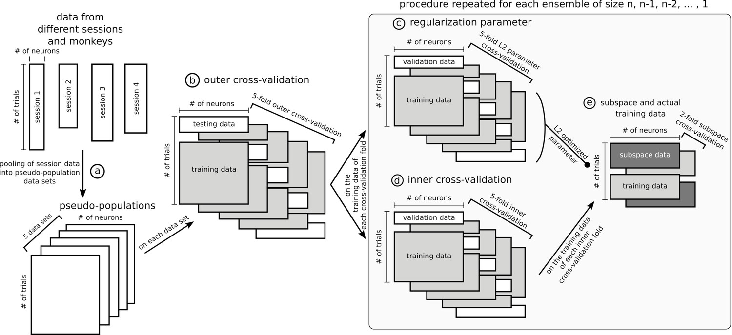
Data sets and cross-validation.
In this figure, data matrices are represented with rectangles where rows are trials and columns units. Data from different sessions were pooled together into pseudo-populations by randomly selecting trials five times so that trial condition was matched (a) and formed five data sets. The rest of the figure represents the specific procedure used to optimize stable ensembles combined with the subspace method, which is the most involved nested cross-validation of the data and was applied independently on each of the five data sets. The outer 5-fold cross-validation (b) ensured that ensembles were not optimized and tested on the same data. The training data in each of the 5 folds of the outer cross-validation was used independently to optimize five stable ensembles (25 total, five data sets times five cross-validation folds). These data were further split following a 5-fold inner cross-validation to train and test a decoder on an ensemble (d) and used in parallel to optimize the L2 normalization parameter of the ridge regression (c), with its own 5-fold cross-validation. To avoid defining the stable subspace and training the ridge decoder on the same data, the training trials from the inner cross-validation were further split in 2, one half for the subspace and the other for the data that were projected into the subspace and then used to train the decoder with the L2 parameter optimized in step (c), and then this split was inversed to allow all data to be either part of the subspace or the training. Note that steps (c), (d) and (e) were repeated for each ensemble tested, from size n-1, n-2,... to a single unit. The ensemble eliciting the most stable representation for each fold of the outer cross-validation was tested on its corresponding test trials of the outer cross-validation. The cross-validation procedure for other analyses was similar but had fewer steps, for example the dynamic ensemble procedure did not involve the subspace/training data split.
Author response image 1
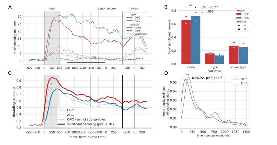
Figure 2, linear value neurons only.
Author response image 2
Figures 3 and 4, linear value neurons only.
Author response image 3
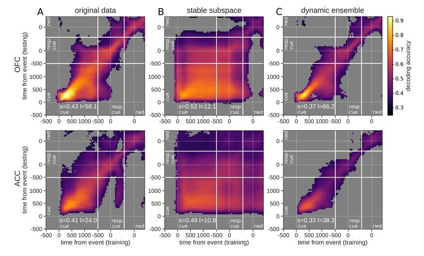
Figure 5, linear value neurons only.
Author response image 4
Tables
Table 1
Number of recorded units with an average activity per session above 1 Hz.
| Single | Multi | Total | |||
|---|---|---|---|---|---|
| Monkey | M | N | M | N | |
| OFC | 259 | 192 | 170 | 177 | 798 |
| ACC | 114 | 72 | 81 | 48 | 315 |
Additional files
Download links
A two-part list of links to download the article, or parts of the article, in various formats.
Downloads (link to download the article as PDF)
Open citations (links to open the citations from this article in various online reference manager services)
Cite this article (links to download the citations from this article in formats compatible with various reference manager tools)
Stable and dynamic representations of value in the prefrontal cortex
eLife 9:e54313.
https://doi.org/10.7554/eLife.54313


