Architecture of the chromatin remodeler RSC and insights into its nucleosome engagement
- University of California, Berkeley, United States
- Lawrence Berkeley National Laboratory, United States
- The Institute for Systems Biology, United States
- Howard Hughes Medical Institute, University of California, Berkeley, United States
Figures
Figure 1 with 9 supplements
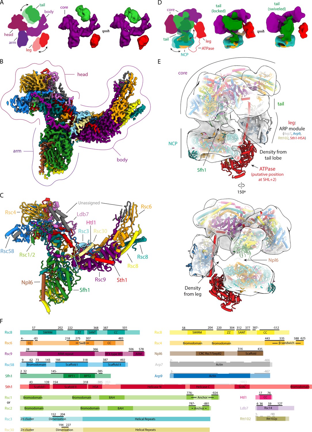
Structures of RSC and RSC-NCP complex.
(A) On the left, cartoon representation of RSC showing its five main lobes. The head, body and arm lobes form the core of the complex, while the tail and leg lobes are flexible. On the right are two cryo-EM reconstructions of RSC with the tail (green) and leg (red) lobes in two different conformations with respect to the core (purple). (B) Cryo-EM reconstruction of the RSC core with individually subunits colored. (C) Model of the RSC core with individual subunits colored and labelled. (D) On the left, cartoon representation of the RSC-NCP complex showing the five main lobes of RSC colored as in A, and with DNA in teal and histones in orange. The tail and leg lobes are flexible. On the right are two cryo-EM reconstructions of RSC-NCP showing the tail lobe in two different conformations with respect to the core. (E) Cryo-EM reconstruction of RSC-NCP in transparent with the core of RSC, the NCP (PDB: 6IY2) (Li et al., 2019) and the ARP module (PDB: 4I6M) (Schubert et al., 2013) structures docked in. The ATPase domain (not visible in our density) is modeled according to the structure of nucleosome-bound Snf2 (PDB: 6IY2) (Li et al., 2019). The points of contact between RSC and the NCP are labeled. (F) Domain maps for RSC subunits. Regions modeled within the RSC core are marked by black lines above the schematic of each protein. The ARP module that was docked into the RSC-NCP map is marked by the dark grey lines and the ATPase domain as shown in the model is marked by light grey lines.
Figure 1—figure supplement 1
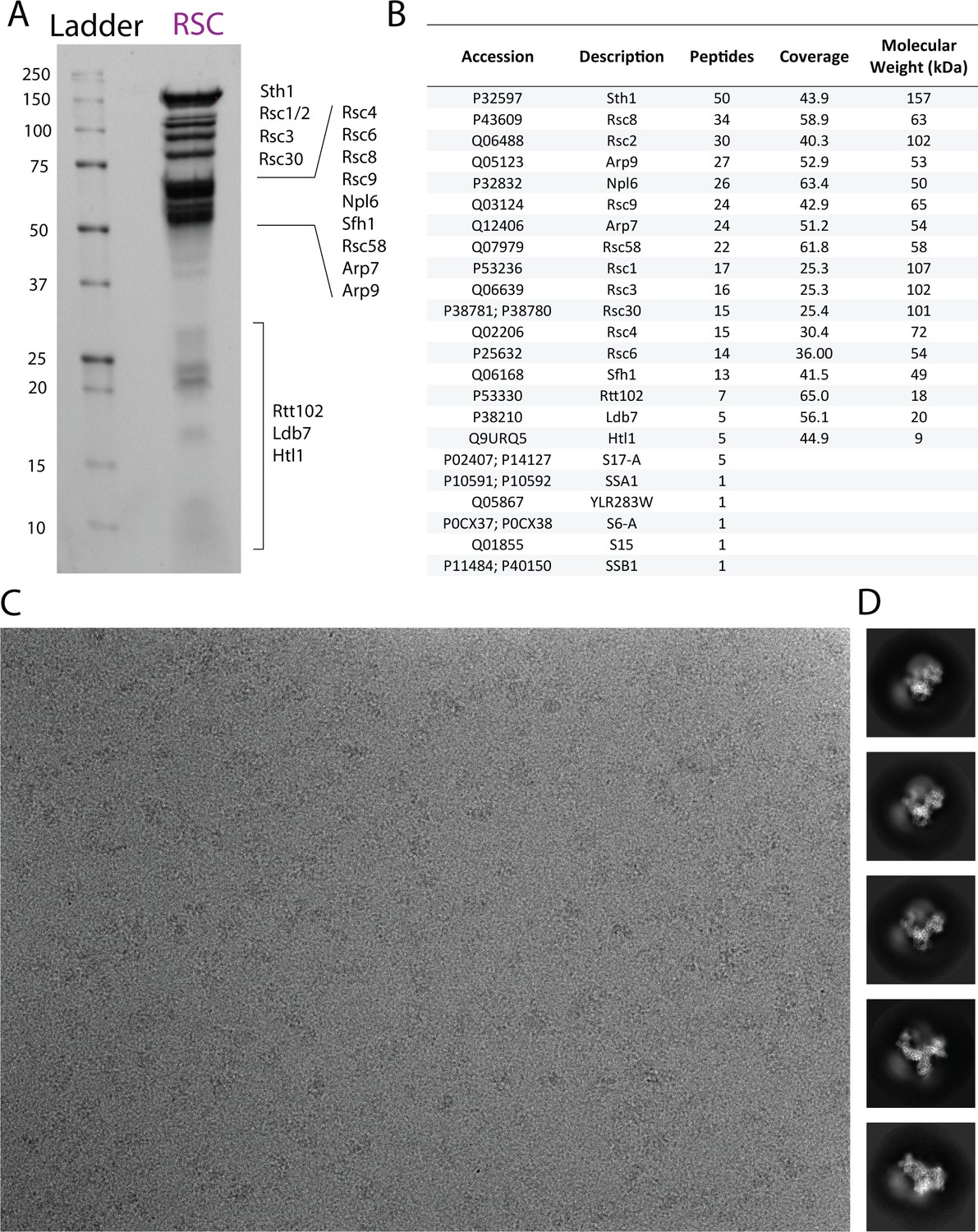
Biochemical Characterization of RSC.
(A) SDS-PAGE (BioRad 4–20%) of purified S. cerevisiae RSC, stained with Flamingo stain. (B) Mass spectrometry analysis showing the presence of all RSC subunits in our sample. (C) Representative cryo-EM micrograph of RSC using open hole grids. (D) Exemplar 2D class averages of apo RSC.
Figure 1—figure supplement 2
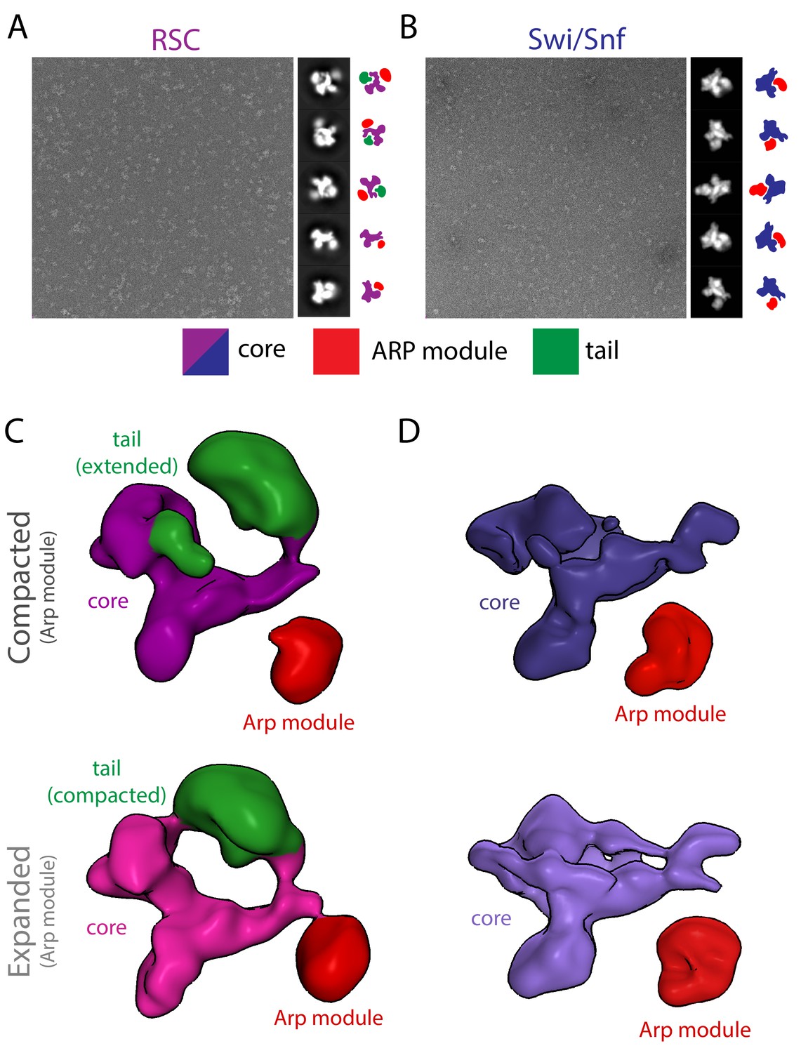
Negative stain analysis of SWI/SNF and RSC.
Negative stain micrograph of RSC (A) and SWI/SNF (B) with 2D class averages and lobe assignment cartoon on the right. The colored cartoons highlight the relative positions of the main lobes (color code at the bottom). Negative stain 3D reconstruction of RSC (C) and SWI/SNF (D), showing that both have a similar looking core and a flexible Arp module.
Figure 1—figure supplement 3
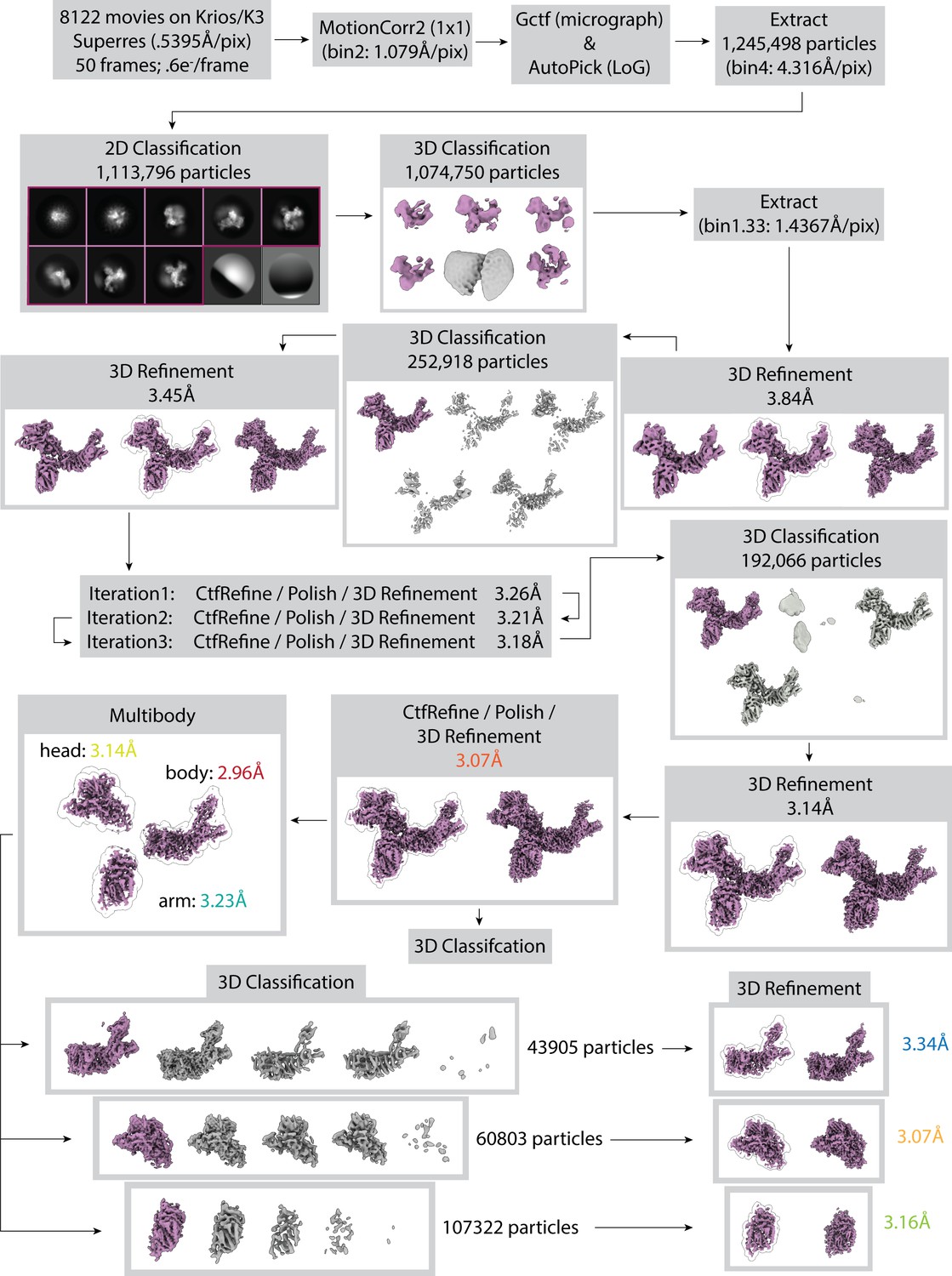
Cryo-EM data collection and processing for apo RSC.
Particles from class averages outlined in purple and 3D classes colored purple were selected for further processing. Particles that went into grey classes were eliminated from further processing. The final global refinement yielded a map with an overall resolution of 3.07 Å for the core. 3D classification without a mask using particles from the 3.07 Å refinement is shown in Figure 3C (tail containing classes are shown in Figure 1A). To improve map quality at the periphery of the core, multibody refinement was performed for the head, arm, and body lobes, followed by 3D classification of the partially signal-subtracted particles. For the arm lobe, a single good class was identified, which was refined to a resolution of 3.16 Å. For the head and body lobes, two distinct good classes were found, with one containing several extra helices. The classes containing the extra density were selected and refined. The head lobe refined to 3.07 Å, and the body refined to 3.48 Å. During the 3D classification steps classes in purple were used for further processing while grey classes were removed. For 3D refinement steps with three maps the results shown are: (left) refinement without a mask, (center) refinement continued with a mask (mask is shown as an outline around map at its highest threshold), and (right) postprocessed map. For 3D refinement steps with two maps the results shown are: (left) refinement with a mask (mask is shown as an outline around map at its highest threshold) and (right) postprocessed map.
Figure 1—figure supplement 4
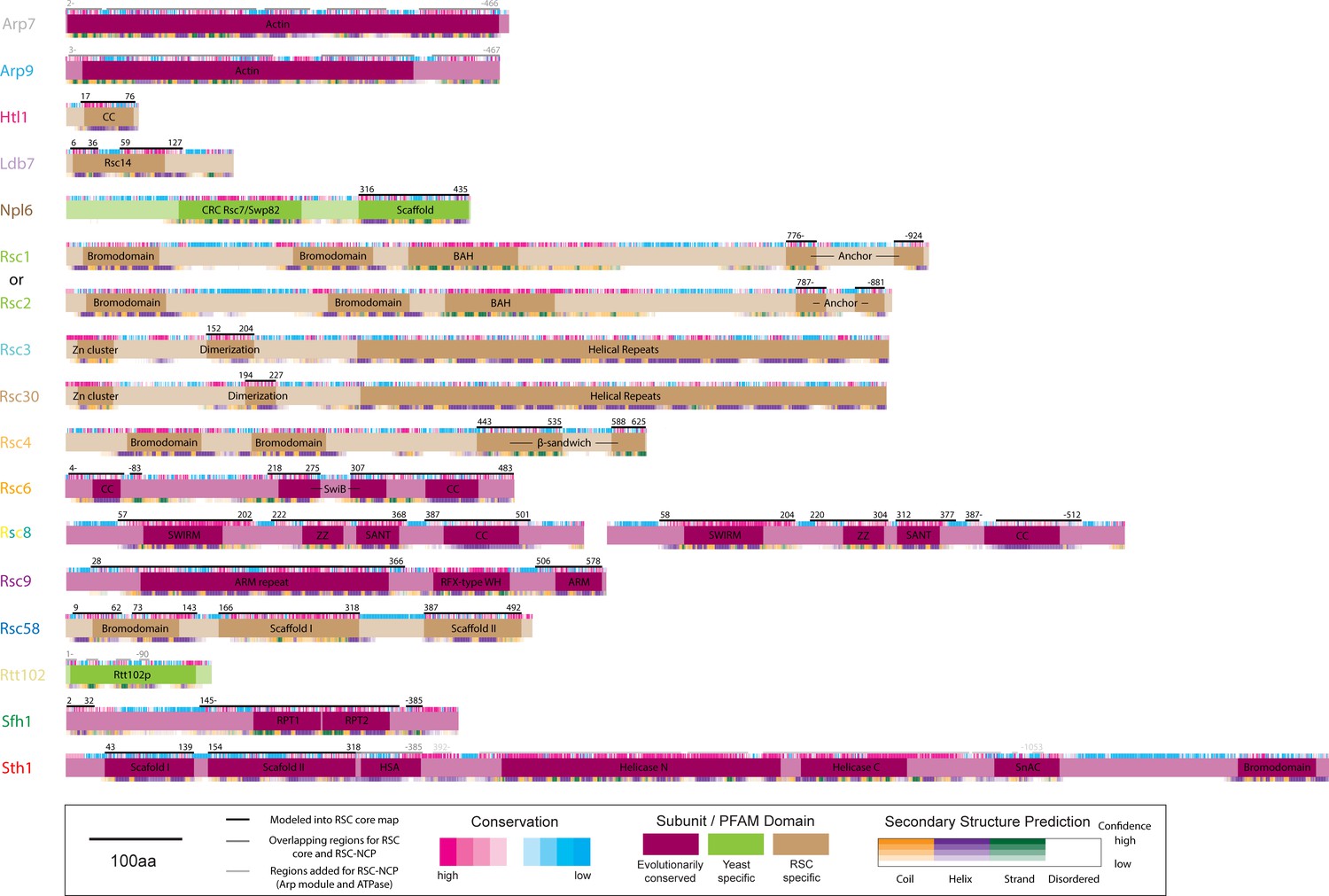
Domain maps of RSC subunits.
Regions modeled within our structure are denoted by a black line above the protein schematic. Conservation scores ranging from high to low (pink to blue) were generated using the Consurf server (Ashkenazy et al., 2010; Ashkenazy et al., 2016). PFAM-predicted domains are labeled in bold (some regions were added and modified based on structural observations). Predicted secondary structure based on PSIPRED and DISOPRED3 results (purple for helix, green for stand, orange for coil and white for disordered) (El-Gebali et al., 2019; Jones, 1999; Buchan et al., 2013; Buchan and Jones, 2019; Jones and Cozzetto, 2015).
Figure 1—figure supplement 5
Modeling of RSC core.
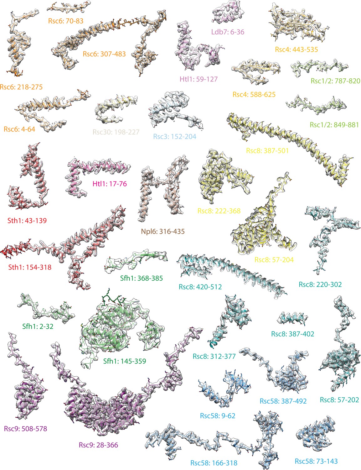
Transparent maps of regions within the RSC core, segmented based on identified chain segments with the built atomic models shown.
Figure 1—figure supplement 6
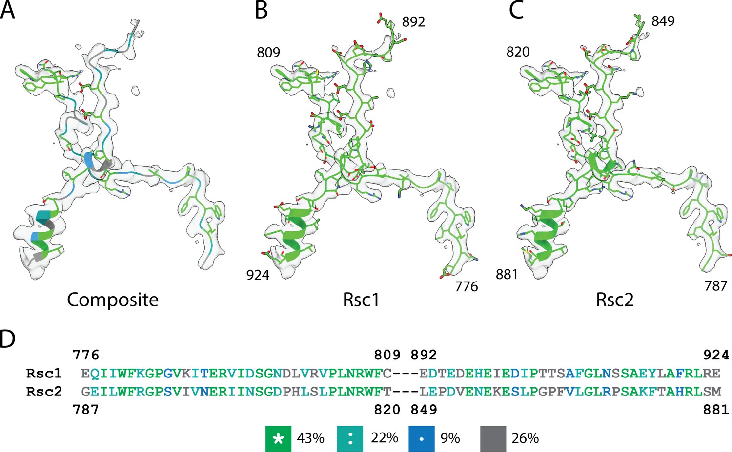
Modeling of Rsc1/2.
(A) Region of the density map assigned to Rsc1/2, with an atomic model showing identical residues between Rsc1 and Rsc2 in green, strongly similar residues in teal, weakly similar residues in blue and dissimilar residues in grey. (B) Model of Rsc1 into the Rsc1/2 density. (C) Model of Rsc2 into the Rsc1/2 density. (D) Sequence alignment of Rsc1 and Rsc2 using Clustal Omega (Sievers et al., 2011), residues are colored according to sequence similarity.
Figure 1—figure supplement 7
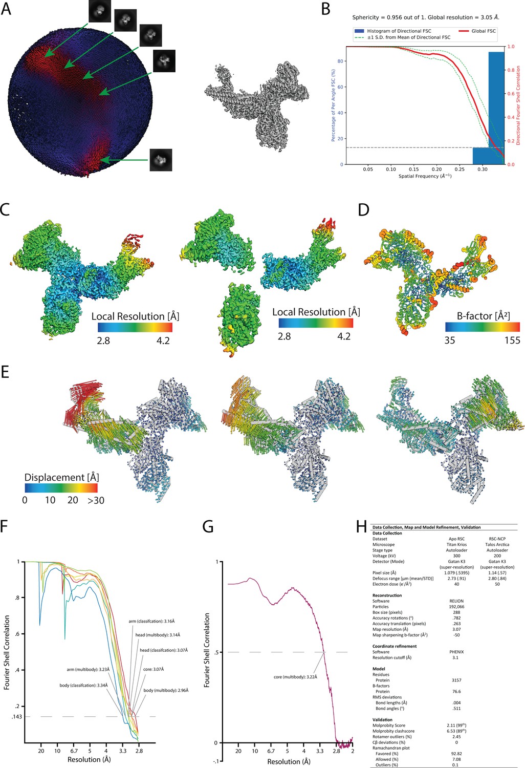
RSC core structure-model validation.
(A) Euler angle distribution (left) for particle images used in the reconstruction of the core of RSC (right). Major orientation peaks are marked with corresponding 2D class averages. (B) 3DFSC plot (Tan et al., 2017) showing isotropic resolution for the core of RSC. (C) Maps for the masked refinement and multibody refinement of the RSC core colored in a rainbow spectrum to represent the local resolution (local resolution calculated using Relion) (Zivanov et al., 2018). (D) Model of the core of RSC colored according to B-Factor. (E) Cα displacement vectors show the motion of the first three principal components of the multibody refinement. The consensus RSC model was flexibly fit into the first and last volumes of the eigenvalue binned structure and Cα displacement vectors were measured from those resulting structures (Lopéz-Blanco and Chacón, 2013). (F) FSC plots for the reconstruction in Figure 1—figure supplement 3. Resolutions are estimated according to the FSC = 0.143 criterion (fully independent reconstructions, gold standard). (G) Model versus map FSC curves for the refined RSC core coordinate model against the summed multibody reconstructions. The FSC = 0.5 criterion indicates a resolution of 3.2 Å for the core of RSC. (H) Refinement table summarizing data collection settings, reconstruction parameters, and model refinement and validation statistics.
Figure 1—figure supplement 8
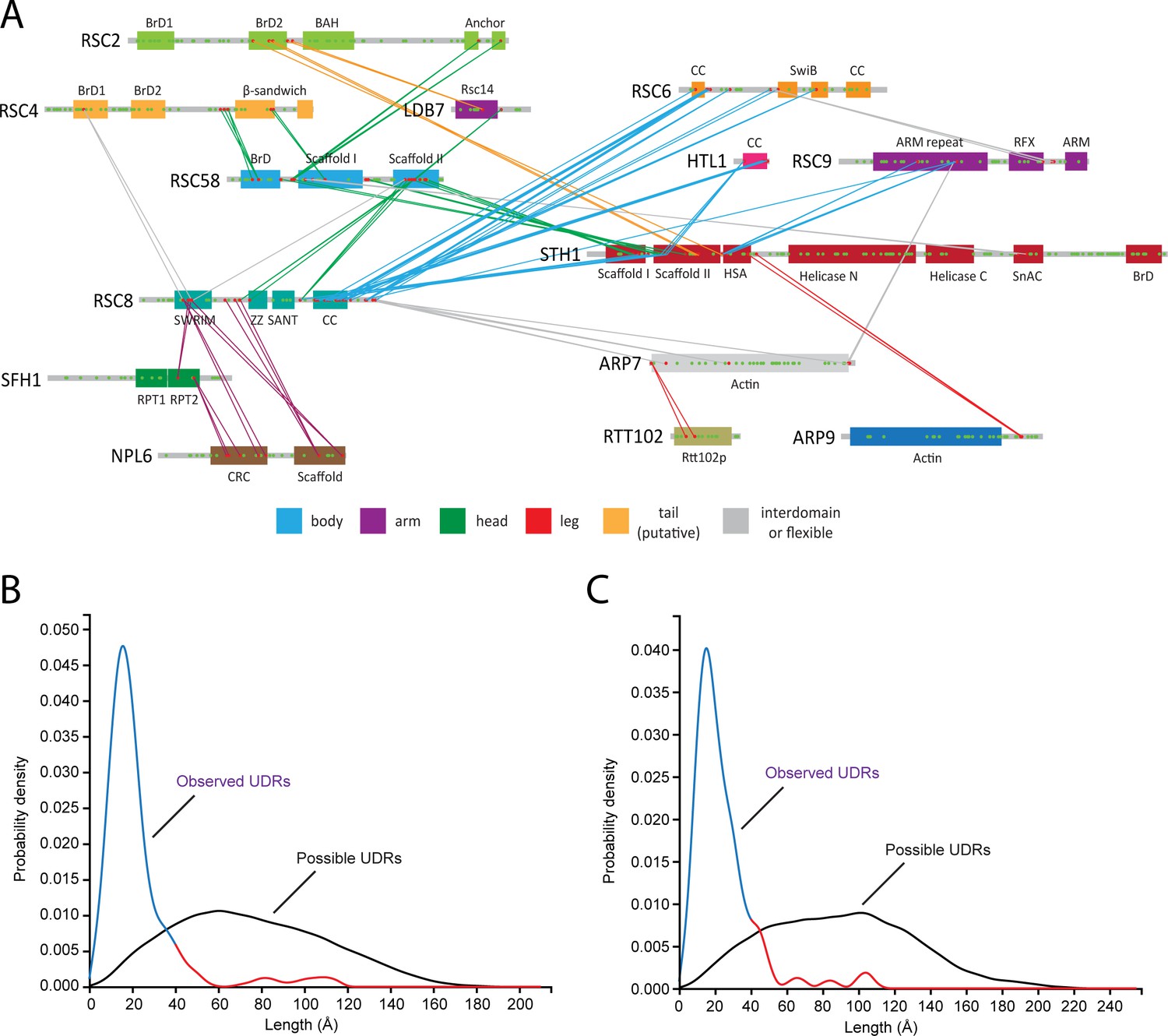
Chemical Crosslinking Mass Spectrometry Analysis of RSC.
(A) Protein-protein crosslinks for the RSC complex, plotted on the domain architecture diagram. Only crosslinks with two or more independent crosslinked peptides within 30 amino acids are shown to simplify the display. Crosslinks are colored based on the lobe that they are within. (B) Probability distribution for the observed and theoretical unique distance restraints (UDRs) for the core of RSC. The observed probability distribution is colored blue (≤38A, possible based on the linker length on BS3) and red (>38A, not possible based on the linker length on BS3). Of the 168 crosslinks that could be mapped onto the structure, 151 (90%) were within 38 Å. (C) Same as (B) but for the RSC core with the Arp module (Arp7, Arp9, Rtt102, and Sth1-HSA). Of the 233 crosslinks that could be mapped onto the structure, 206 (88%) were within 38 Å.
Figure 1—figure supplement 9

Cryo-EM data collection and processing for the RSC-NCP complex.
Data processing workflow. Particles from class averages outlined in purple and 3D classes colored purple were selected for further processing. Particles that went into grey classes were eliminated from further processing. The final global refinement yielded a map with an overall resolution of 19 Å for RSC bound to a NCP. Further classification showed that the tail region shifts towards the NCP in a subset of particles.
Figure 2
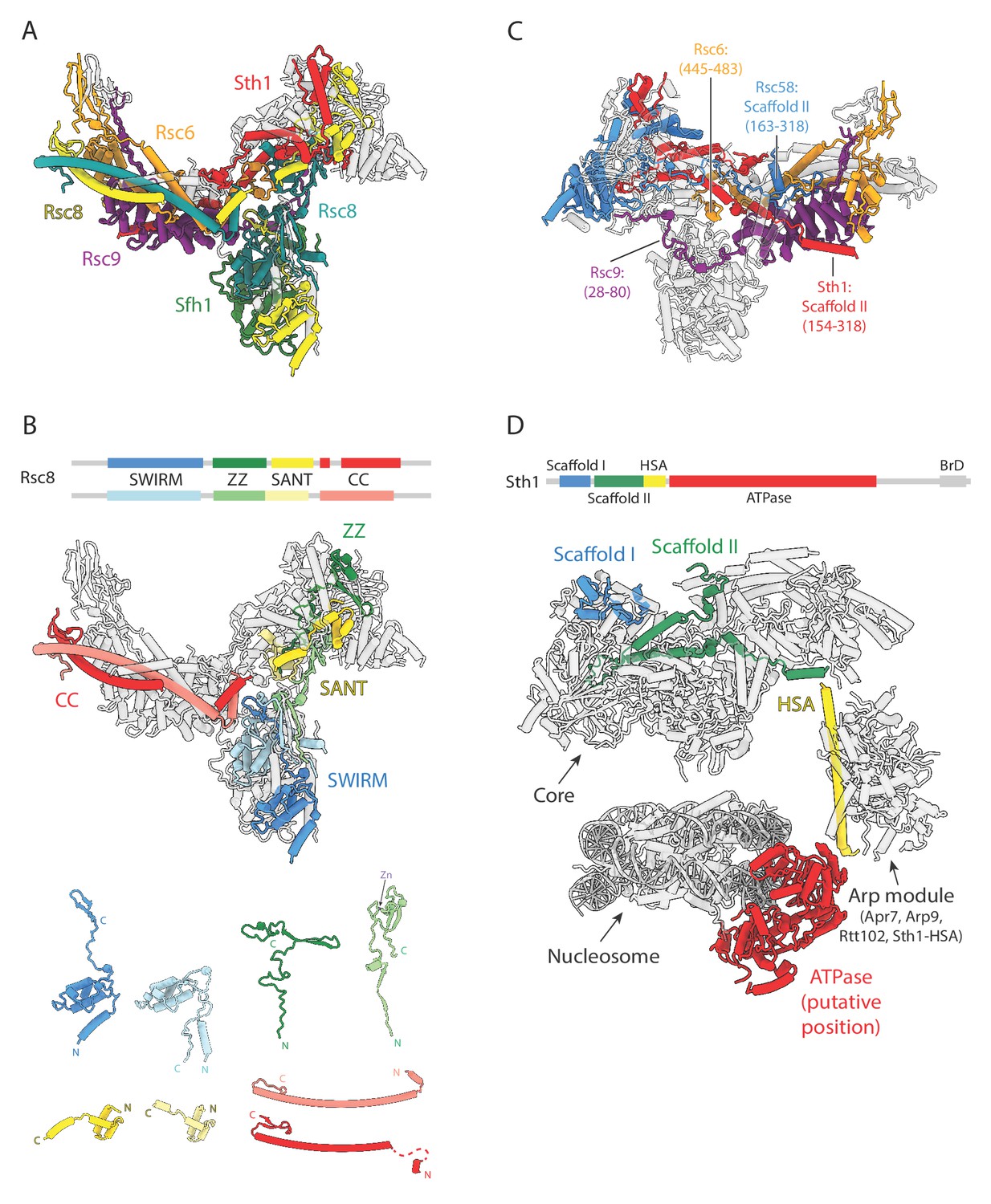
Conserved structural scaffold in RSC.
(A) Structure of the RSC core, highlighting in color the evolutionarily conserved subunits. Non-conserved subunits are shown in transparent grey. Subunit labels are shown with colors corresponding to those in the structure. (B) Top, domain map of Rsc8, with the four different domains colored blue to red from N to C terminus. Middle, structure of the RSC core with only the Rsc8 dimer colored. Bottom, individual domains of the two copies of Rsc8, aligned and tiled. (C) RSC subunits that span multiple lobes (except for Rsc8) are colored, with the regions spanning them labeled. (D) Model of the RSC-NCP complex with domains of Sth1 highlighted blue to red from N to C terminus. Scaffolding domains I (blue) and II (green) interact with the core region of RSC, while the HSA helix (yellow) interacts with the Arp module to form the leg lobe. The ATPase (red; not visible in our density) is modeled according to the structure of nucleosome-bound Snf2 (ref. Li et al., 2019).
-
Figure 2—source data 1
SWI/SNF family of chromatin remodelers.
Table of subunit homology for complexes in yeast and humans.
- https://cdn.elifesciences.org/articles/54449/elife-54449-fig2-data1-v2.docx
Figure 3
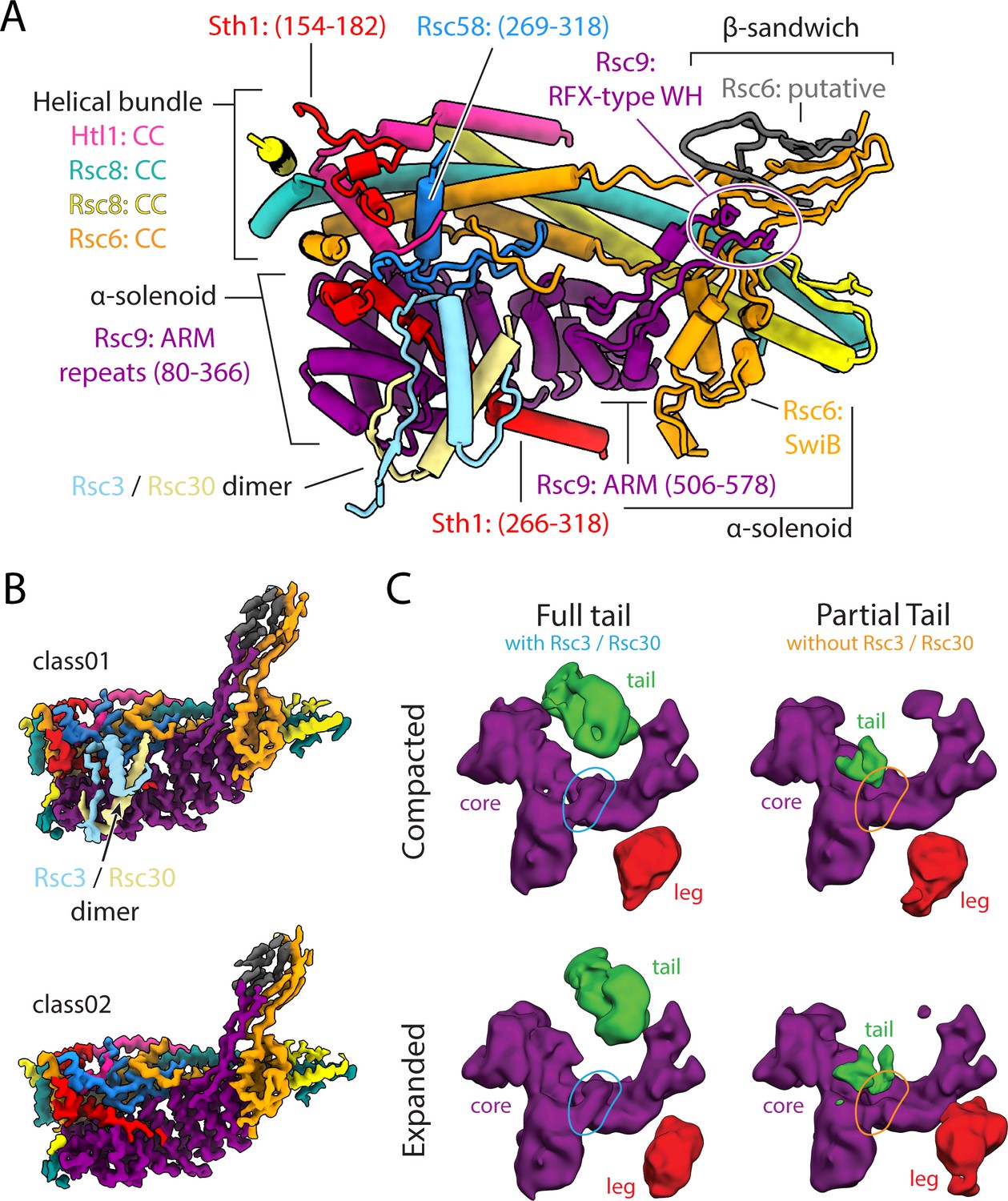
Architecture of the body lobe and occupancy of the tail lobe.
(A) Structure of the RSC body lobe, with protein domains and segments labeled. (B) Two maps generated from 3D classification of the body region. Shown is the presence or absence of RSC3/30 density with the body lobe. Maps were generated using partial signal subtraction and 3D classification. (C) Four classes generated from 3D classification using the final high-resolution set of particles, without mask and with a reference that was low pass filtered to 20 Å at every iteration. These classes reveal the flexibility of the tail and leg lobes of RSC and correlate the presence of the tail lobe with the Rsc3/Rsc30 occupancy in the core.
Figure 4
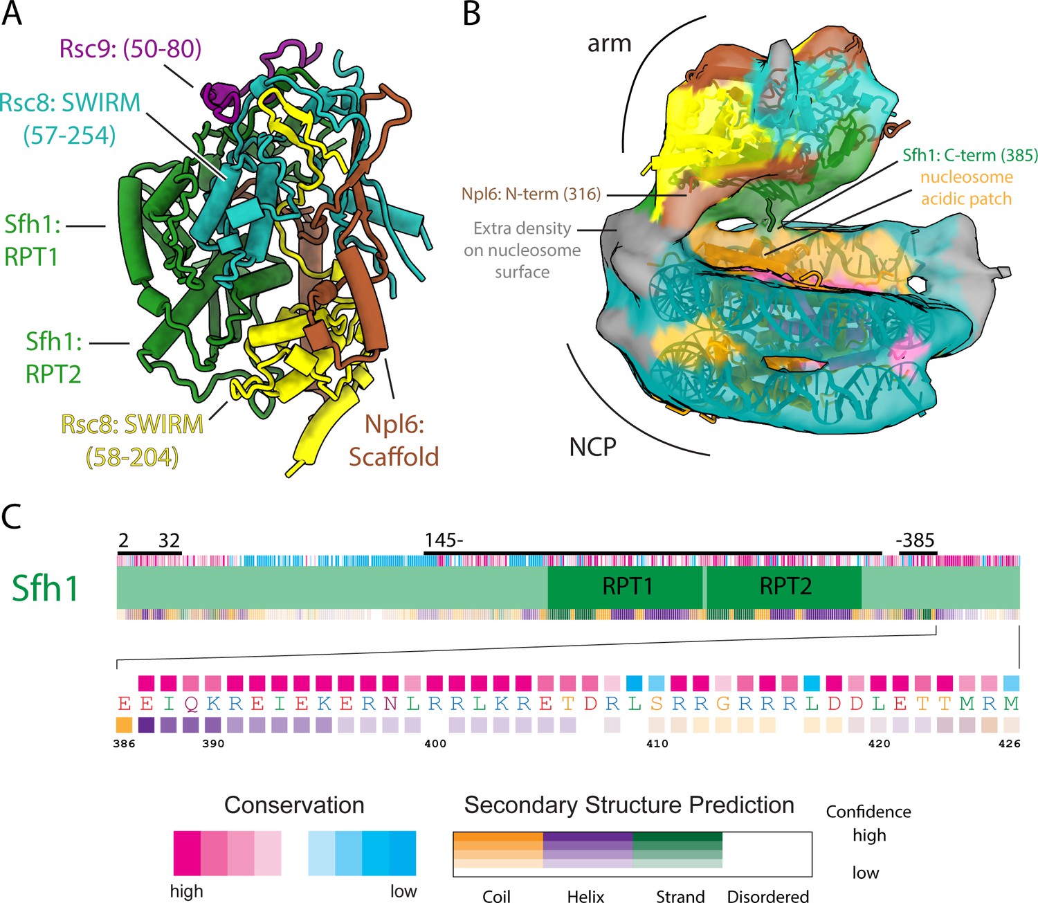
Architecture of the arm lobe and is interaction with the NCP.
(A) The structure of the RSC arm lobe with protein domains and segments labeled. (B) The density of the NCP and arm region from the RSC-NCP reconstruction showing the connections that occur between the two. (C) Domain organization, sequence conservation and secondary structure prediction for Sfh1. Below is a zoomed in view of the C-terminus showing the sequence at a residue level. The domain map coloring is the same as in (Figure 1—figure supplement 4).
Figure 5
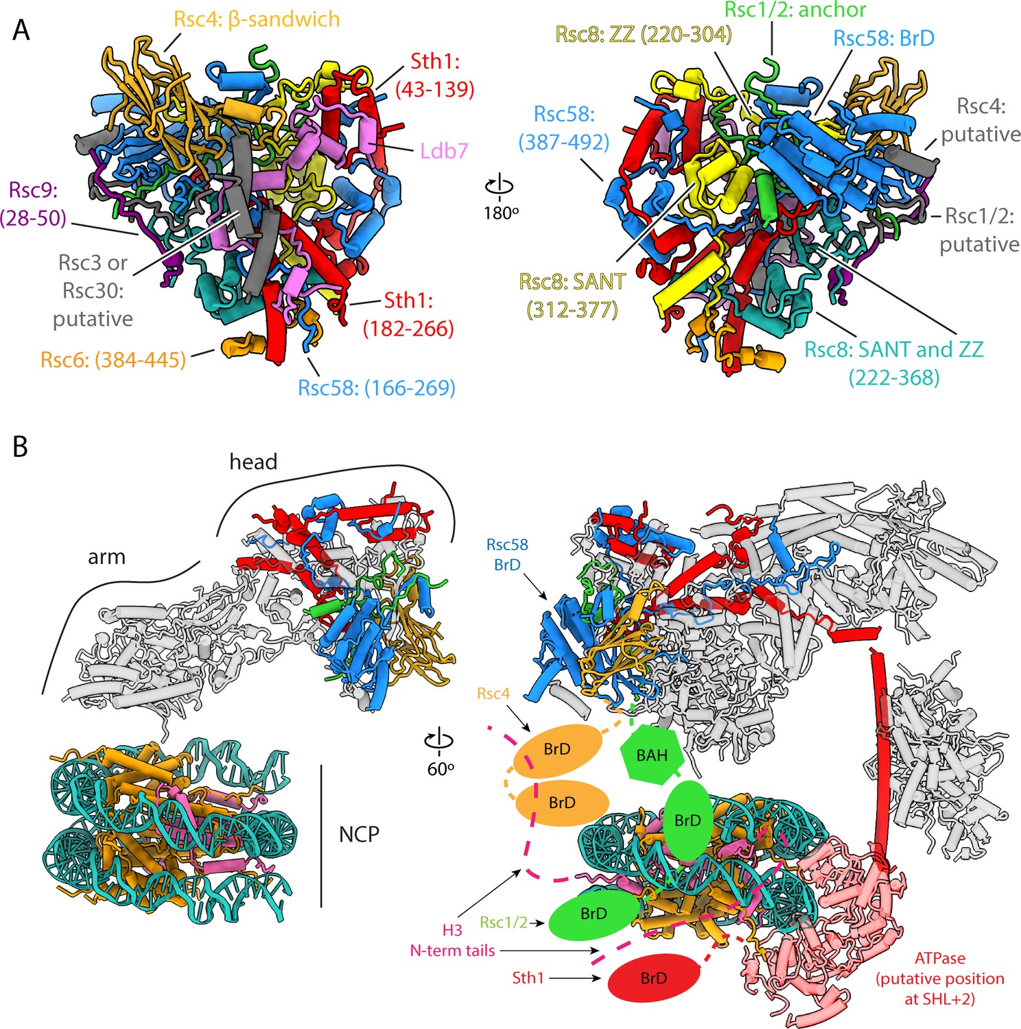
Architecture of the head lobe, the chromatin reader hub.
(A) Structure of the RSC head lobe with protein domains and segments labeled. (B) On the left the RSC-NCP model showing the head lobe situated over the top of the nucleosome. On the right in the full RSC-NCP model with cartoon connections for the chromatin interacting domains (BrDs and BAH) shown. Only the RSC subunits that contain chromatin interacting domains are colored. The nucleosome is colored teal for DNA, orange for histones H2A, H2B and H4, and pink for H3.
Figure 6
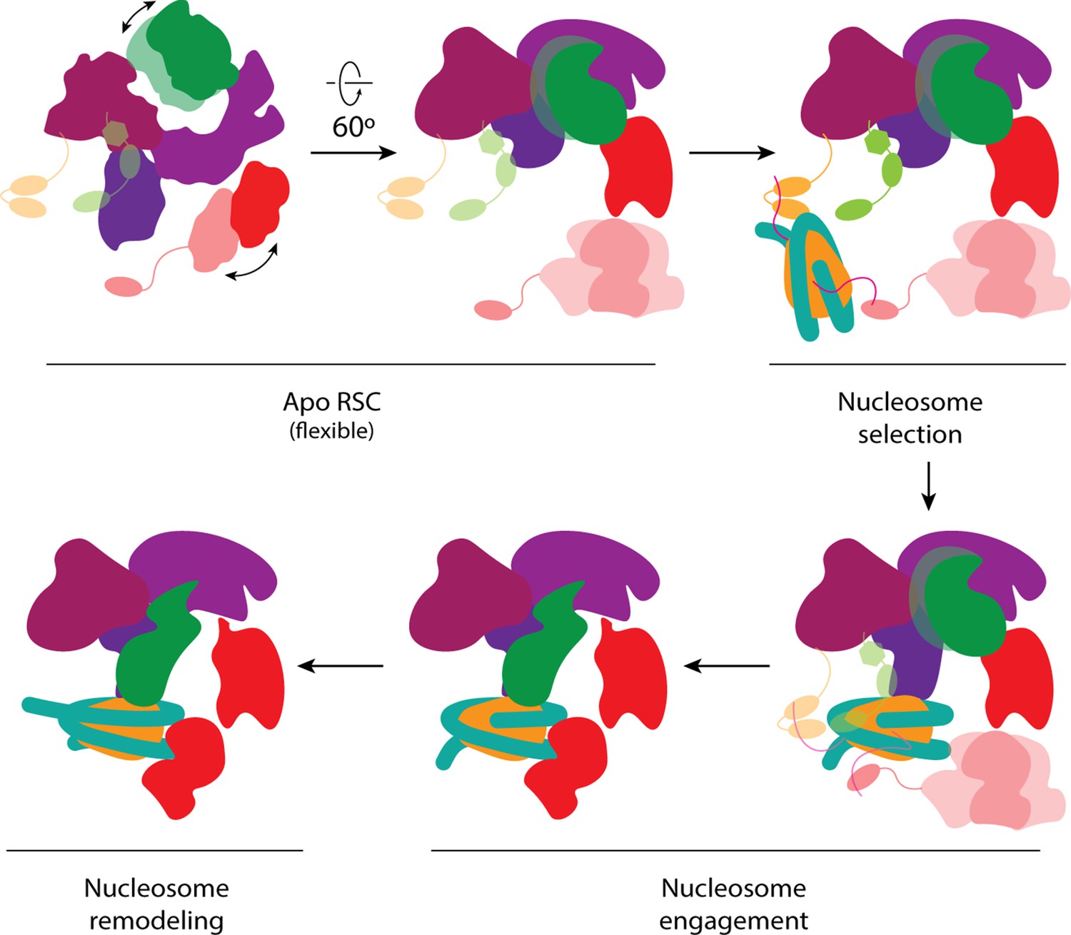
Proposed model of nucleosome engagement.
Mechanistic model of RSC engaging a nucleosome. The apo RSC is shown with its moving tail and leg lobes, and its flexibly attached histone-tail binding domains. The BrDs bind and select target nucleosomes with acetylated tails. The selected nucleosome engages RSC, first through the arm lobe of the core, which then positions the ATPase domain at the end of the leg to be able to bind SHL2. During nucleosome remodeling, the ATPase translocates the DNA while the RSC core holds onto the histone core.
Figure 7

Proposed model of RSC assembly.
Proposed assembly process of RSC highlighting the individual, initial stages, which involve only evolutionarily conserved subunits.
Appendix 1—figure 1 with 1 supplement
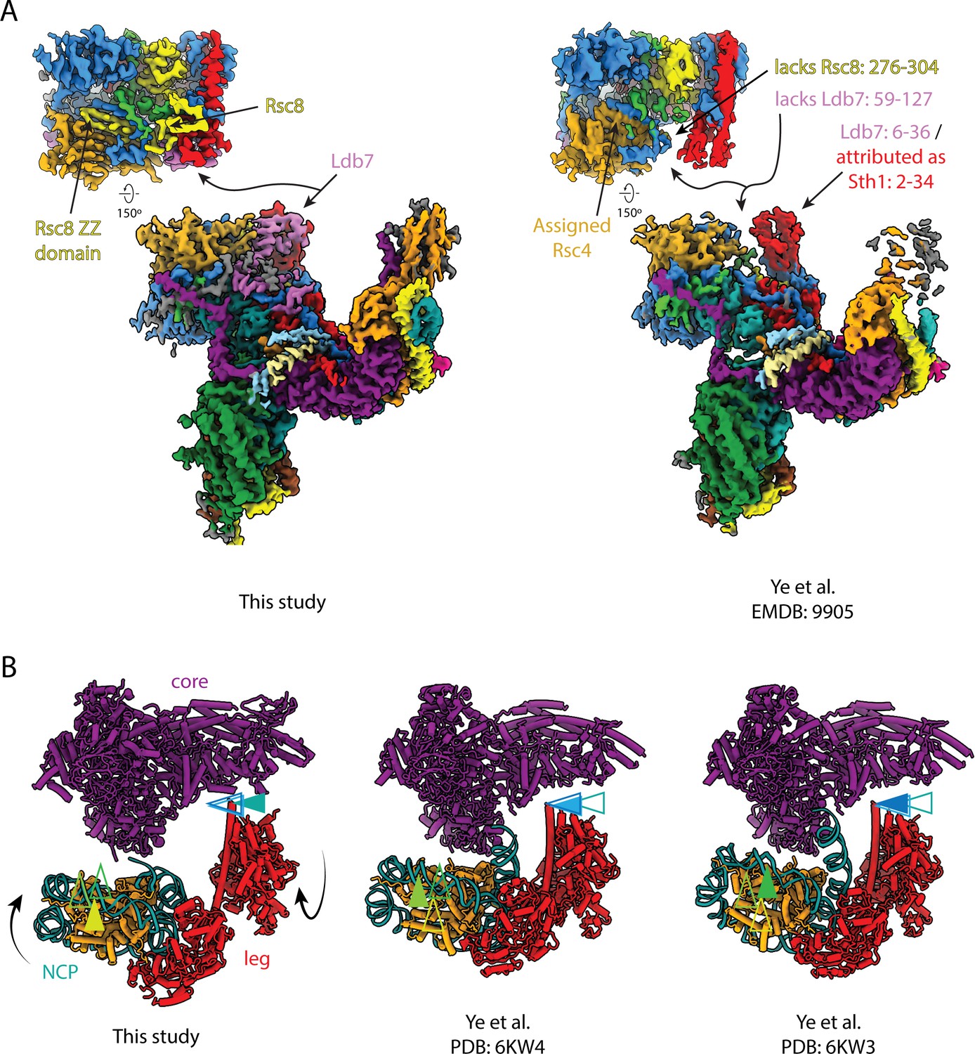
Structural comparison of RSC complexes.
(A) Structures of the RSC core from this study (left) and (Ye et al., 2019) (right) . (B) Structures of the RSC core from this study (left) and (Ye et al., 2019) (middle and right). Arrows indicate relative positions of nucleosome super-helical location 0 (SHL0) (yellow-green) and HSA helix (teal-blue).
Appendix 1—figure 1—figure supplement 1
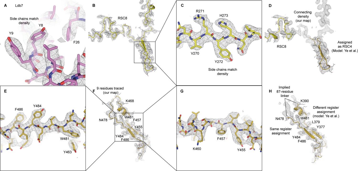
Interpretation of densities for Ldb7, Rsc8 and Rsc4.
(A) Fit of our model of Ldb7 model in our map (this study). Key side chains used in assignment are labeled. (B) Trace of Rsc8 (model and map shown from this study), with side chain fits highlighted (C). (D) Same map region from (B) but fitting model from Ye et al. (F) Trace of Rsc4 β-strands (model and map shown from this study), with side chain fits highlighted (E, G). (H) Same map region from (H) but fitting model from Ye et al.
Additional files
Download links
A two-part list of links to download the article, or parts of the article, in various formats.
Downloads (link to download the article as PDF)
Open citations (links to open the citations from this article in various online reference manager services)
Cite this article (links to download the citations from this article in formats compatible with various reference manager tools)
Architecture of the chromatin remodeler RSC and insights into its nucleosome engagement
eLife 8:e54449.
https://doi.org/10.7554/eLife.54449


