A compositional neural code in high-level visual cortex can explain jumbled word reading
- Centre for BioSystems Science & Engineering, Indian Institute of Science, India
- Department of Electrical Communication Engineering, Indian Institute of Science, India
- Centre for Neuroscience, Indian Institute of Science, India
Figures
Figure 1
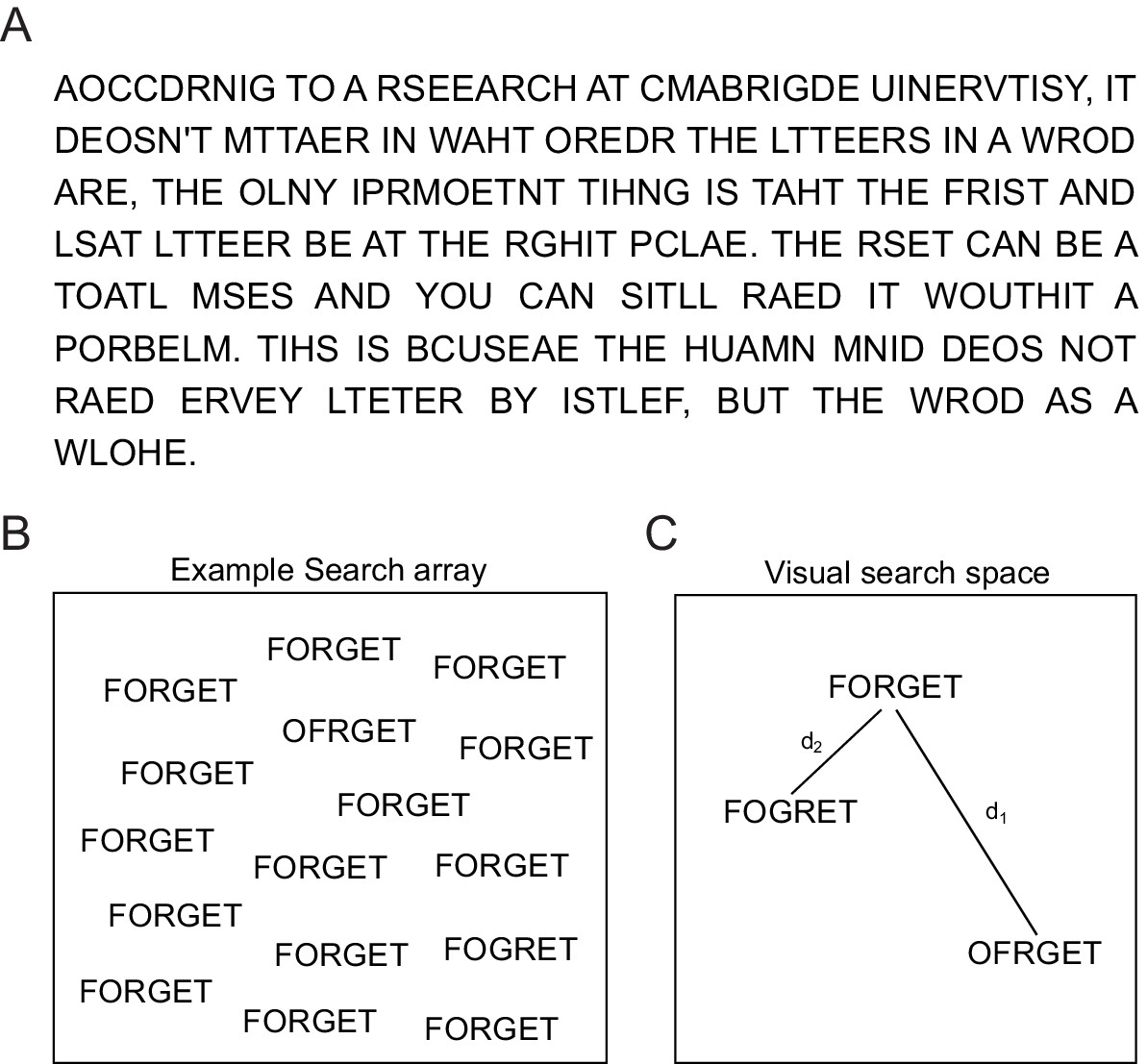
Reading jumbled words.
(A) We are extremely good at reading jumbled words, as illustrated by the popular Cambridge University effect. (B) Visual search array showing two oddball targets (OFRGET and FOGRET) among many instances of FORGET. OFRGET is easy to find but not FOGRET. (C) Schematic representation of these strings in visual search space, arranged such that similar items (corresponding to harder searches) are nearby. Thus, FOGRET is visually more similar to FORGET compared to OFRGET (i.e. d1 > d2). This makes FOGRET easy to recognize as FORGET compared to OFRGET.
Figure 2
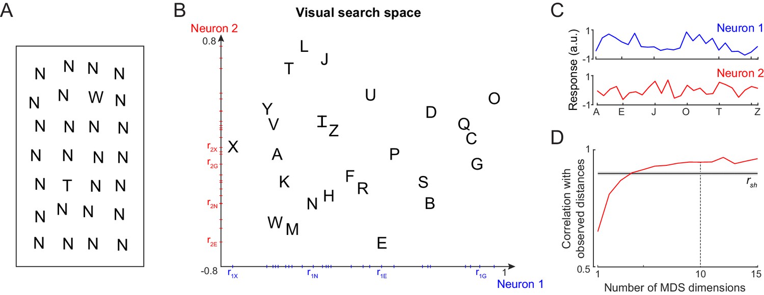
Single letter discrimination (Experiment 1).
(A) Visual search array showing two oddball targets (W and T) among many Ns. It can be seen that finding W is harder compared to finding T. The actual experiment comprised search arrays with only one oddball target among 15 distractors. (B) Visual search space for uppercase letters obtained by multidimensional scaling of observed dissimilarities. Nearby letters represent hard searches. Distances in this 2D plot are highly correlated with the observed distances (r = 0.82, p<0.00005). Letter activations along the x-axis are taken as responses of Neuron 1 (blue), and along the y-axis are taken as Neuron 2 (red), etc. The tick marks indicate the response of each letter along that neuron. (C) Responses of Neuron 1 and Neuron 2 shown separately for each letter. Neuron 1 responds best to O, whereas Neuron 2 responds best to L. (D) Correlation between observed distances and MDS embedding as a function of number of MDS dimensions. The black line represents the split-half correlation with error bars representing s.d calculated across 100 random splits.
Figure 3
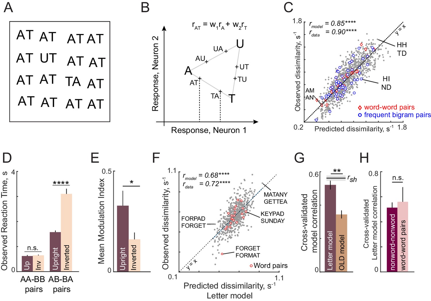
Discrimination of strings is explained using single letters (Expts 2–4).
(A) Example search array with two oddball targets (UT and TA) among the bigram AT. It can be seen that UT is easier to find than TA, showing that letter substitution causes a bigger visual change compared to transposition. (B) Schematic diagram of how the bigram response is obtained from letter responses. Consider two neurons selective to single letters A, T and U. These letters can be represented in a 2D space in which the response to each neuron lies along one axis. For each neuron, we take the response to a bigram to be a weighted sum of the single letter responses. Thus, the bigram response lies along the line joining the two stimuli. Note that the bigrams AT and TA can be distinguished only if there is unequal summation. In the schematic, the first position is taken to have higher magnitude, as a result of which the response to AT is closer to A than to T. (C) Observed dissimilarities between bigram pairs plotted against predictions of the letter model for word-word pairs (red diamonds), frequent bigram pairs (blue circles) and all other bigram pairs (gray dots), for Experiment 2. Model correlation is shown at the top left, along with the data consistency for comparison. Asterisks indicate the statistical significance of the correlations (**** is p<0.00005). (D) Average observed search reaction time for upright (dark) and inverted (pale) bigram searches for repeated letter pairs (AA-BB pairs) and transposed letter pairs (AB-BA pairs) in Experiment 3. Asterisks indicate statistical significance of the main effect of orientation in an ANOVA (see text for details; **** is p<0.00005). (E) Mean modulation index of the summation weights, calculated as |w1-w2|/|w1+w2|, where w1 and w2 are the bigram summation weights, averaged across the 10 neurons in the letter model for upright (dark) and inverted (pale) bigrams. The asterisk indicates statistical significance calculated on a sign-rank test comparing the modulation index across 10 neurons (* is p<0.05). (F) Observed dissimilarities between six-letter strings in visual search (Experiment 4) plotted against predicted dissimilarities from the single letter model for word-word pairs (red dots) and all other pairs (gray dots). Model correlation is shown at the top left with data consistency for comparison. Asterisks indicate statistical significance of the correlations (**** is p<0.00005). (G) Cross-validated model correlation for the letter model (dark) and the Orthographic Levenshtein distance (OLD) model (light). For each model, the cross-validated correlation is the correlation between model predictions trained on one half of the data and the observed response times from the other half. The upper bound on model fits is the split-half correlation (rsh) shown in black with shaded error bars representing standard deviation across 1000 random splits. The asterisk indicates statistical significance of the comparison obtained by estimating the fraction of bootstrap samples in which the observed difference was violated (** is p<0.005). (H) Cross-validated letter model correlation for word-word pairs and nonword-nonword pairs.
Figure 4

Lexical decision task behavior (Experiment 5).
(A) Schematic of visual word space, with one stored word (PENCIL) and two nonwords (PENICL and EPNCIL). We hypothesize that subjects would take longer to categorize a nonword when it is similar to a word, that is RT for PENICL would be larger than for EPNCIL. Thus, 1/RT would be proportional to this dissimilarity. Likewise we predicted that subjects would be faster to respond to frequent words which have a stronger stored representation. (B) Response times for words in the lexical decision task, sorted in descending order. The solid line represents the mean categorization time for words and the shaded bars represent s.e.m. Some example words are indicated using dotted lines. The split-half correlation between subjects (rsh) is indicated on the top. (C) Cross-validated model correlation between observed and predicted word response times across all words for various models: log word frequency (blue), number of orthographic neighbors (orange), log mean bigram frequency (purple), log mean letter frequency (cyan) and a combined model containing all these factors (red). Shaded error bars indicate mean ± sd of the correlation across 1000 random splits of the observed data. The asterisk indicates statistical significance of the comparison obtained by estimating the fraction of bootstrap samples in which the observed difference was violated (* is p<0.05, ** is p<0.005). (D) Response times for nonwords in the lexical decision task, sorted in descending order. Conventions as in (A). (E) Observed reciprocal response times for nonwords in the lexical decision task plotted against letter model predictions fit to the full data (450 nonwords). Some example nonwords are depicted. (F) Percent change in response time (nonword-RT – word-RT)/word-RT for middle and edge letter transpositions and for middle and edge substitutions for observed data (left) and for letter model predictions (right). MS: middle substitution. In both cases, asterisks represent statistical significance comparing the means of the corresponding groups using a rank-sum test (* is p<0.05, ** is p<0.005, etc.). (G) Observed reciprocal response times plotted against the Orthographic Levenshtein Distance (OLD), a popular model for edit distance between strings. (H) Cross-validated model correlation between observed and predicted nonword RTs for the letter model, OLD model, lexical model and the combined neural+lexical model. Conventions are as in (B).
Figure 5
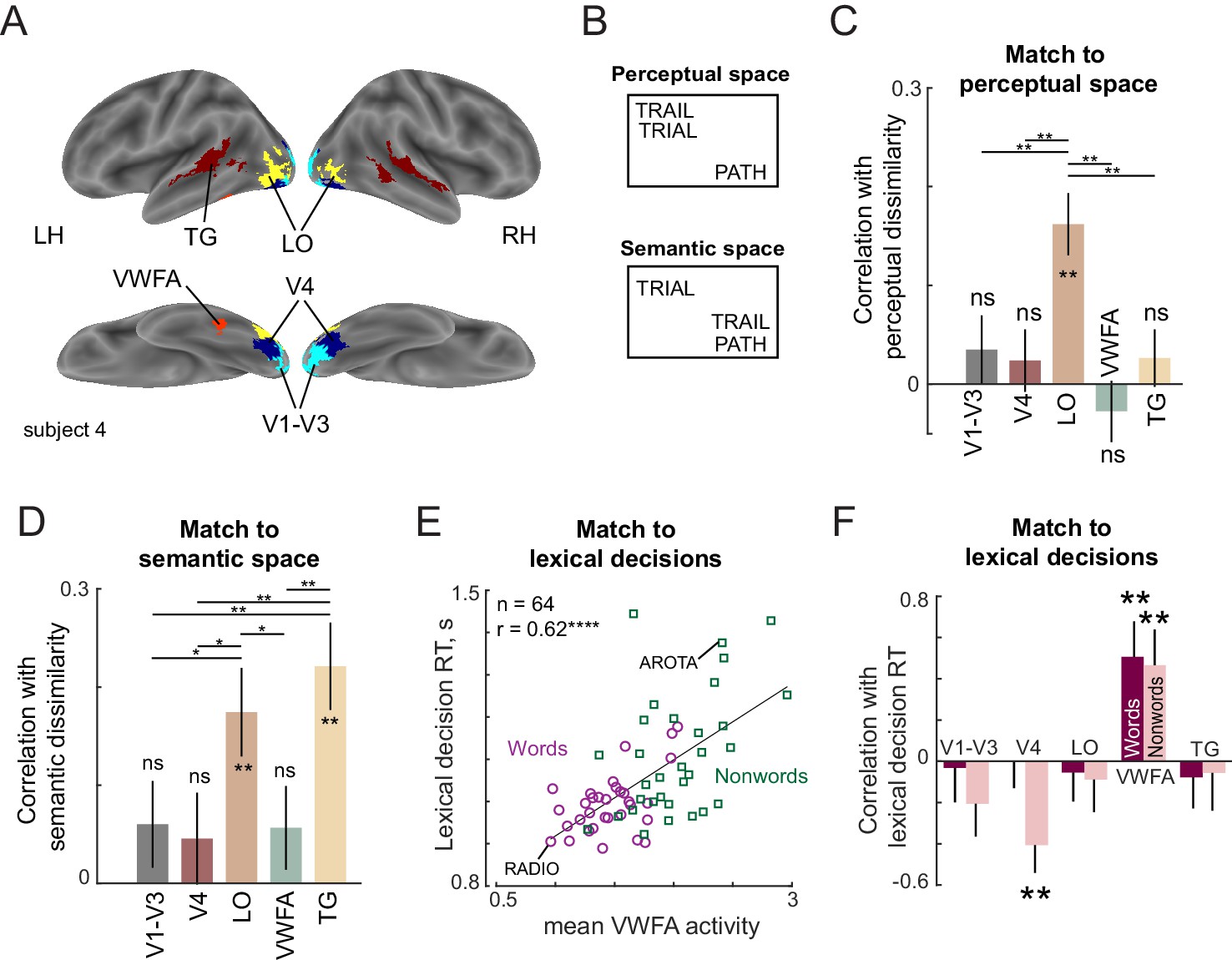
Lexical task fMRI (Experiment 6).
(A) ROIs for an example subject, showing V1–V3 (cyan), V4 (blue), LO (yellow), VWFA (red) and TG (maroon). (B) Example difference between perceptual and semantic spaces. In perceptual space, the representation of TRAIL is closer to its visual similar counterpart TRIAL, whereas in semantic space, its representation is closer to its synonym PATH. (C) Correlation between neural dissimilarity in each ROI with perceptual dissimilarity between strings measured using visual search (Experiment 7). Error bars indicate standard deviation of the correlation between the group perceptual dissimilarity and ROI dissimilarities calculated repeatedly by resampling of dissimilarity values with replacement across 1000 iterations. Asterisks along the length of each bar indicate statistical significance of the correlation between group behavior and group ROI dissimilarity (** is p<0.005 across 1000 bootstrap samples). Horizontal lines indicate the fraction of bootstrap samples in which the observed difference was violated (* is p<0.05, ** is p<0.005, etc.). All significant comparisons are indicated. (D) Correlation between neural dissimilarity in each ROI with semantic dissimilarity for words. Other details are same as in (C). (E) Correlation between mean VWFA activity (averaged across subjects and voxels) with mean lexical decision time for both words (purple circles) and nonwords (green squares). Each point corresponds to one string and example word and nonword is highlighted. Asterisks indicate statistical significance (**** is p<0.00005). (F) Correlation between lexical decision time and mean activity within each ROI separately for words and nonwords. Error bars indicate standard deviation across 1000 bootstrap splits. Asterisks indicate statistical significance (** is p<0.005).
Figure 6
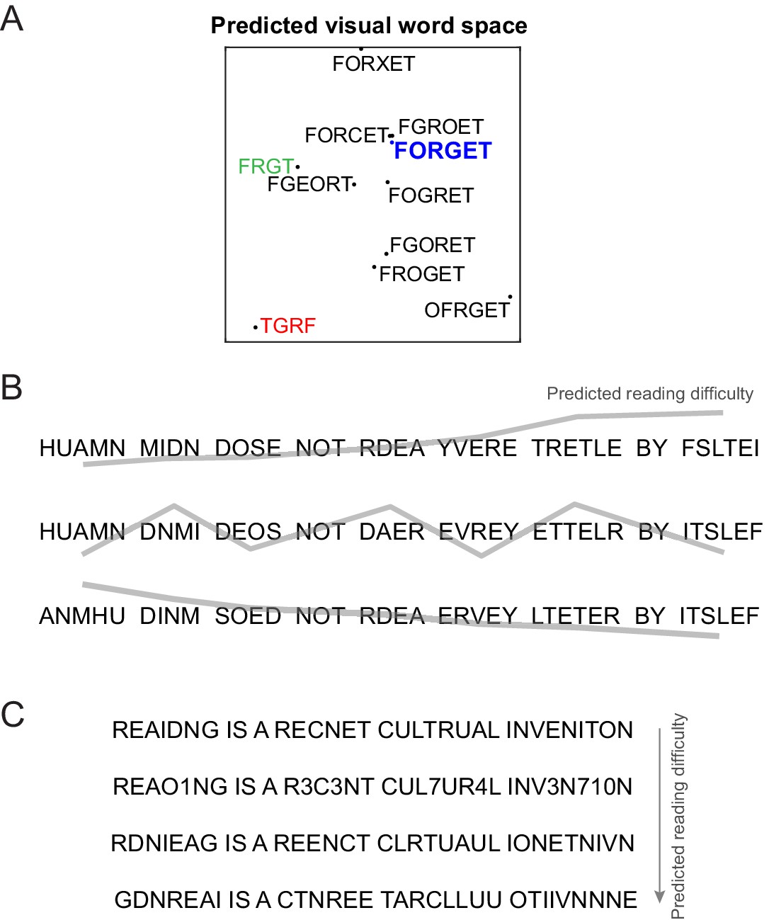
Predicting reading difficulty using the letter model.
(A) Visual word space predicted by the letter model for a word (FORGET) and its jumbled versions. Letter model predictions were based on training the model on compound words (Experiment 4). The plot was obtained by performing multidimensional scaling on the pairwise dissimilarities between strings predicted by the letter model. It can be seen that classic features of orthographic processing are captured by the letter model, including priming effects such as FRGT (green) being more similar to FORGET than TGRF (red). (B) The letter model can be used to sort jumbled words by their reading difficulty, allowing us to create any desired reading difficulty profile along a sentence. Top row: Sentence with increasing reading difficulty. Middle row: sentence with fluctuating reading difficulty. Bottom row: sentence with decreasing reading difficulty. (C) The letter model yields a composite measure of reading difficulty that combines letter substitution and transposition effects. Sentences with digit substitutions (second row) can thus be placed along a continuum of reading difficulty relative to other sentences (first, third and fourth rows) with increasing degree of scrambling.
Appendix 1—figure 1
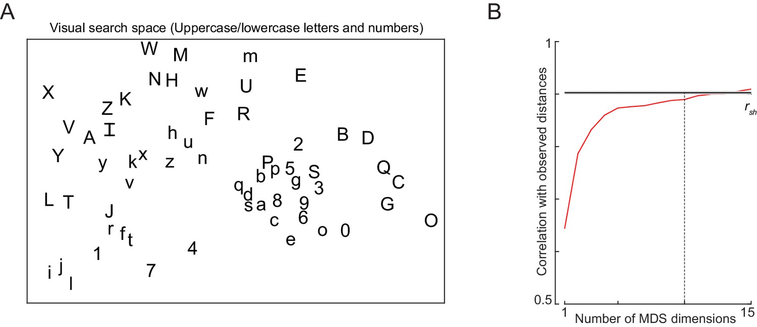
Visual search space for letters and digits.
(A) Visual search space for letters (uppercase and lowercase) and digits obtained by multidimensional scaling of observed dissimilarities. Nearby letters represent hard searches. Distances in this 2D plot are highly correlated with the observed distances (r = 0.79, p<0.00005). (B) Correlation between observed distances and MDS embedding as a function of number of MDS dimensions. The horizontal line represents the split-half correlation with error bars representing s.d calculated across 100 random splits.
Appendix 2—figure 1
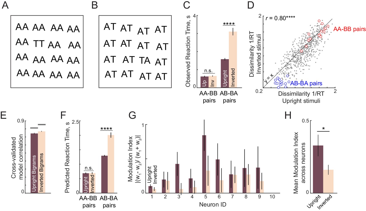
Letter model fits for upright and inverted bigrams.
(A) Example oddball search array for a repeated letter target (TT) among identical repeated-letter distractors (AA). It can be seen that inverting this search array does not affect search difficulty. (B) Example oddball search array for transposed letters (TA among AT). It can be seen by inverting this search array makes the search substantially more difficult. (C) Average search times in the oddball search task for repeated-letter searches (AA-BB) and transposed letter (AB-BA) searches. Error bars represent s.e.m calculated across subjects. Asterisks represent statistical significance (**** is p<0.00005), as obtained using an ANOVA on the response times with subject, bigram and orientation as factors (see text). (D) Dissimilarity of inverted bigram pairs plotted against the dissimilarity of upright bigram pairs. Correlation is shown at the top left. Asterisks indicate statistical significance of the correlations (**** is p<0.00005). (E) Cross-validated model correlation of the letter model for upright bigrams and inverted bigrams. Shaded gray bars represent the upper bound achievable in each case given the consistency of the data, calculated using the split-half correlation rsh. (F) Predicted RT from the letter model for repeated letter pairs and transposed letter pairs. Asterisks denote statistical significance as obtained using a sign-rank test on the predicted RTs between upright and inverted conditions. (G) Spatial modulation index for each neuron in the letter model for upright and inverted bigrams. (H) Average spatial modulation index for upright and inverted bigrams. Asterisks represent statistical significance (* is p<0.05) obtained using a sign-rank test on the spatial modulation index across the 10 neurons.
Appendix 2—figure 2
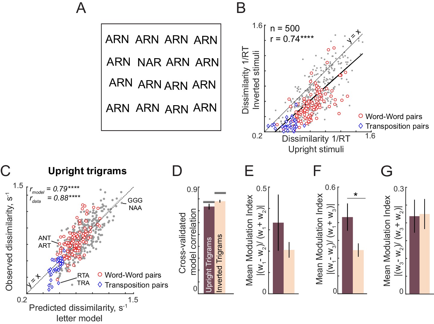
Letter model fits for upright and inverted trigrams.
(A) Example trigram search array containing letter transpositions, with oddball target (NAR) among distractors (ARN). It can be seen that this search is substantially harder when inverted compared to upright. (B) Dissimilarity for inverted trigram searches (1/RT) plotted against dissimilarity for upright trigram searches for word-word pairs (red circles, n = 105), transposed letter pairs (blue diamonds, n = 30), and other pairs (gray circles, n = 365). (C) Observed dissimilarity for upright trigrams plotted against the predicted dissimilarity from the letter model with symbol conventions as in (B). (D) Cross-validated letter model correlation for upright and inverted trigrams. (E) Average spatial modulation index (across 10 neurons) for the first and second letters in the trigram. (F) Same as (E) but for the first and third letters. (G) Same as (E) but for the second and third letters.
Appendix 3—figure 1
Stimulus set used for Experiment 4 (Compound Words).
The left and the right three letters words were combined to form a six-letter string. The strings that formed compound words are highlighted in red.
Appendix 3—figure 2
Visual search for compound words (Experiment 4).
(A) Three-letter words (top) used to create compound words (bottom). (B) Illustration of letter and trigram models. In the letter model, the response to a compound word is a weighted sum of responses to the six single letters. In the trigram model, the response to a compound word is a weighted sum of its two trigrams. (C) Observed dissimilarity for compound words plotted against predicted dissimilarity from the letter model for word pairs (red) and other pairs (gray). (D) Cross-validated model correlations for the letter model, trigram model and the Orthographic Levenshtein distance (OLD) model. The upper bound on model fits is the split-half correlation (rsh), shown in black with shaded error bars representing standard deviation across 30 random splits. Horizontal lines above shaded error bar depicts significant difference across different models. (E) Cross-validated model fits of the letter model for word-words pairs and nonword-nonword pairs. (F) Observed dissimilarities for three-letter words (black) and nonwords (red) plotted against letter model predictions.
Appendix 3—figure 3
Spatial summation weights for each neuron.
Estimated spatial summation weights (mean ±std across many random starting points of the nonlinear model fit algorithm) for each neuron in the letter model.
Appendix 4—figure 1
Letter model performance for varying length strings.
For each experiment, we obtained a cross-validated measure of model performance using six neurons as follows: each time we divided the subjects randomly into two halves, and trained the letter model on one half of the subjects and tested it on the other half. This was repeated for 30 random splits. The correlation between the model predictions and the average dissimilarity from the held-out half of the data was taken to be the model fit. The correlation between the observed dissimilarity between the two random splits of subjects is then the upper bound on model performance (mean ±std shown as gray shaded bars).
Appendix 5—figure 1
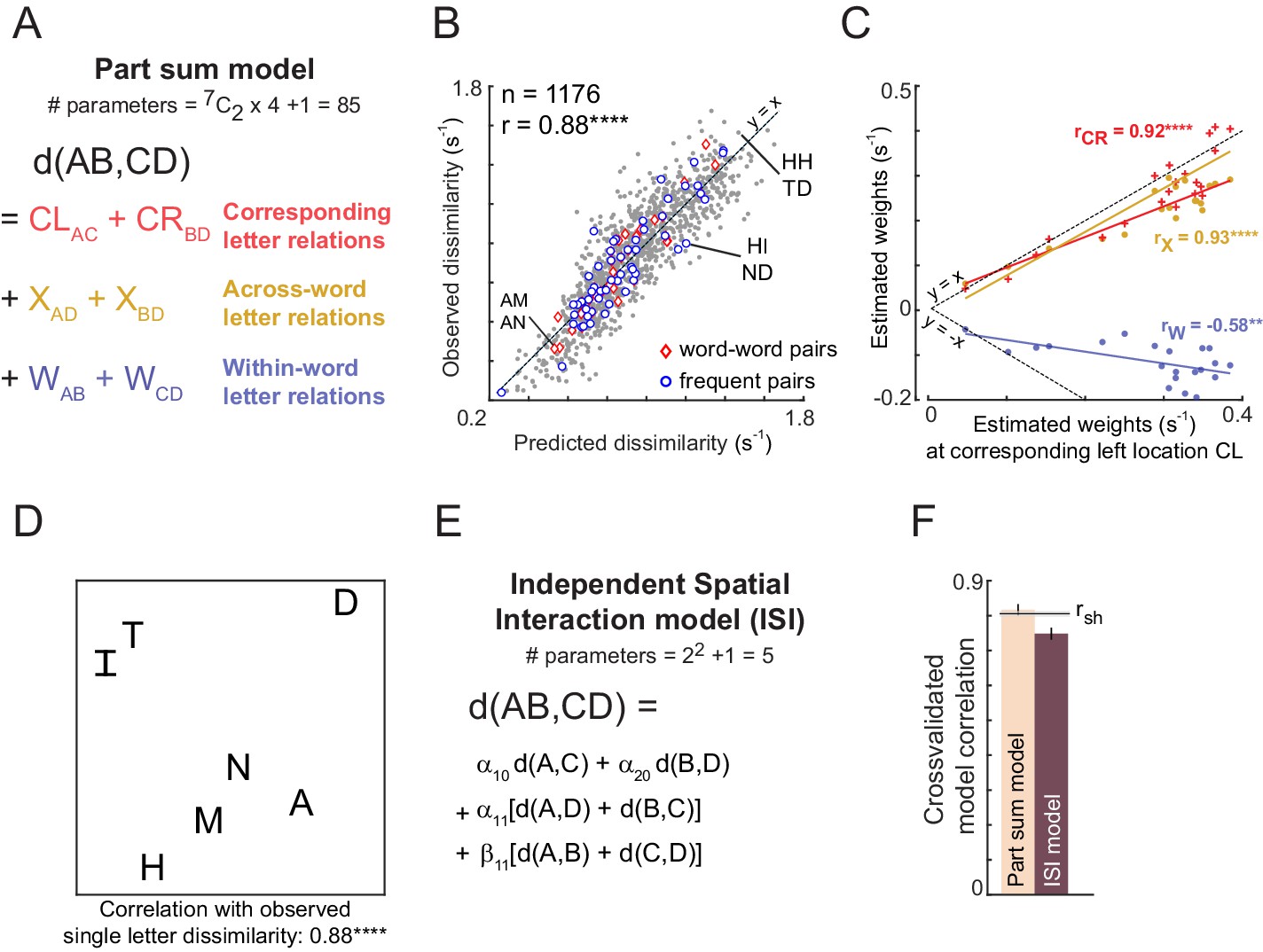
Predicting bigram dissimilarity using part-sum model.
(A) Schematic of the part sum model. According to this model, the dissimilarity (1/RT) between bigrams ‘AB’ and ‘CD’ is written as a linear sum of dissimilarities of its corresponding part terms (AC and BD, shown in red), across part terms (AD and BC, shown in yellow), and within part terms (AB and CD, shown in blue). (B) Correlation between the observed and predicted dissimilarities (1/seconds). Each point represents one search pair (n = 49C2=1176). Word-word pairs are highlighted using red diamonds, and frequent bigram pairs are highlighted using blue circles. Dotted lines represent unity slope line. (C) Correlation between the estimated weights at corresponding location left with estimated weights at 1) corresponding location right (red), 2) across location (yellow), and 3) within location (blue). Each point represents one letter pair (n = 7C2=21). Dotted lines represent positive and negative unity slope line. (D) Perceptual space of the single letter dissimilarities, that are the model coefficients of part terms at left corresponding location (E) Schematic of the Independent Spatial Interaction model. In this model, we use the observed letter-pair dissimilarities and only estimate the weights of these letter-pair dissimilarities across different locations. (F) Comparing part-sum and ISI model fits. Bar plots represents mean correlation coefficient between the observed and predicted dissimilarities. Error bars represent one standard deviation across 30 splits. Black horizontal line represents mean split-half correlation (rsh) and the shaded error bar represents one standard deviation around the mean. (****, p<0.00005, **, p<0.005).
Appendix 5—figure 2
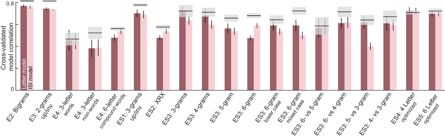
ISI and letter model performance across all experiments.
For each experiment, we obtained a cross-validated measure of both neural and ISI model performance as follows: each time we divided the subjects randomly into two halves, and trained the letter model on one half of the subjects and tested it on the other half. This was repeated for 30 random splits. The correlation between the model predictions and the average dissimilarity from the held-out half of the data was taken to be the model fit. The correlation between the observed dissimilarity between the two random splits of subjects is then the upper bound on model performance (mean ±std shown as gray shaded bars).
Appendix 5—figure 3
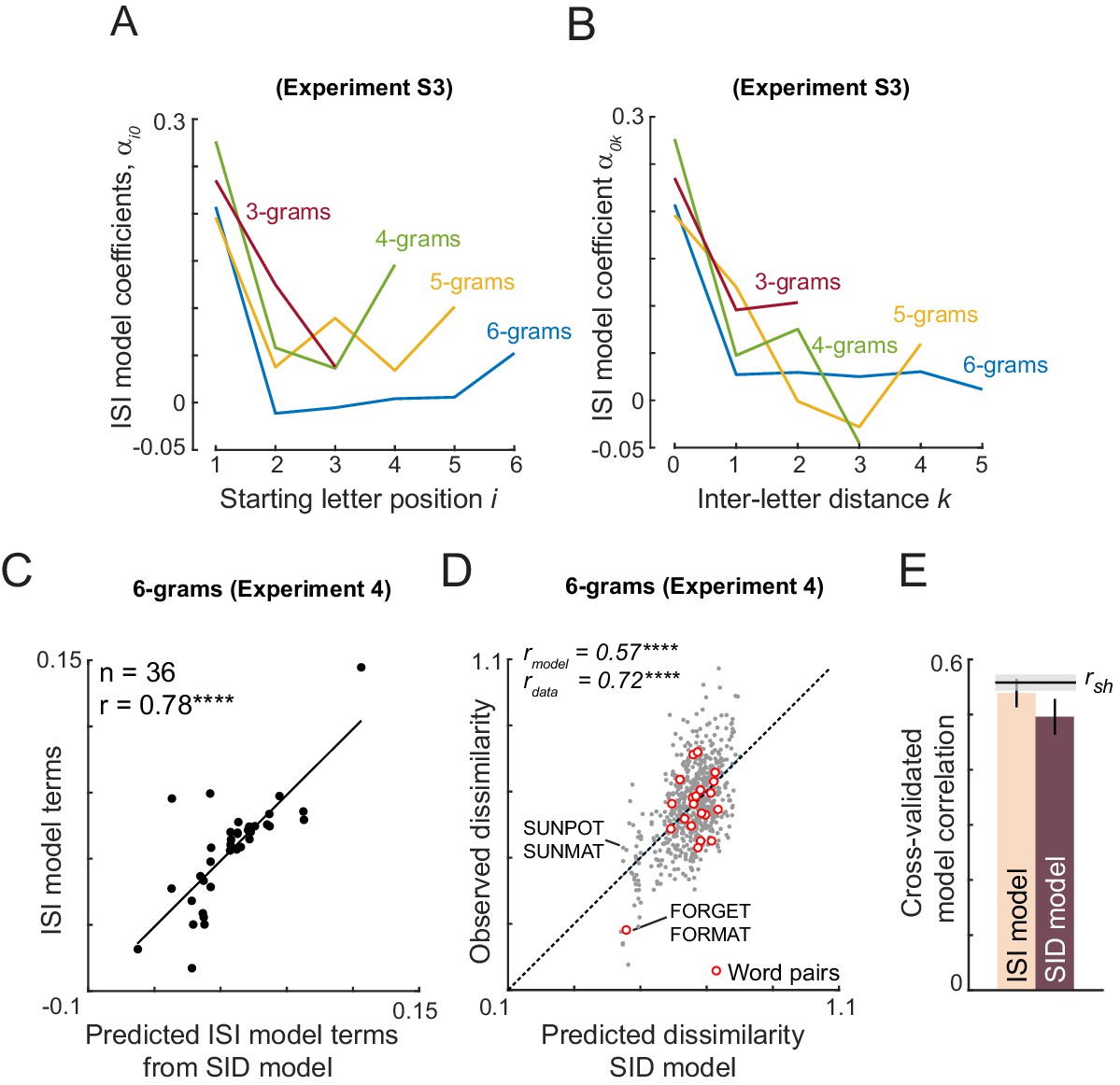
Reducing the ISI model.
(A) ISI model coefficients as a function of starting letter position i, for Experiment S3, for varying string lengths. (B) ISI model coefficients as a function of inter-letter distance k for Experiment S3, for varying string lengths. (C) ISI model coefficients (both αik and ) plotted against the predicted ISI model coefficients from the SID model. Both models are fitted to data from Experiment 4 (compound words). (D) Observed dissimilarity in Experiment four plotted against predicted dissimilarity from the SID model. (E) Cross-validated model correlation for ISI and SID models.
Appendix 5—figure 4
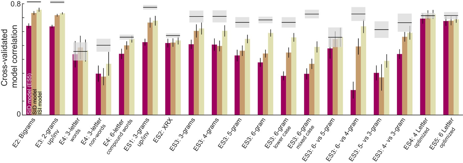
ISI and SID model fits across all experiments.
Cross-validated model fits for the ISI and SID models across all experiments. In each case the SID and ISI models were fit on a randomly chosen half of the subjects and tested on the other half. The SID (ES5) bars refer to the SID model trained on Experiment S5 and tested on data from a randomly chosen half of subjects in each experiment.
Appendix 5—figure 5
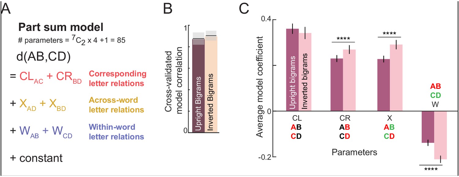
Part-sum model fits for upright and inverted bigrams.
(A) Schematic of the part-sum model, in which the net dissimilarity between two bigrams is given as a linear sum of letter dissimilarities at corresponding locations (CL and CR), across-bigrams (X) and within-bigrams (W). (B) Cross-validated model correlation of the part sum model for upright and inverted bigrams. (C) Average model coefficients (mean ±sem) of each type for upright and inverted bigrams. Asterisks denote statistical significance (**** is p<0.00005) obtained on a sign-rank test comparing 15 letter dissimilarities between upright and inverted conditions).
Appendix 5—figure 6
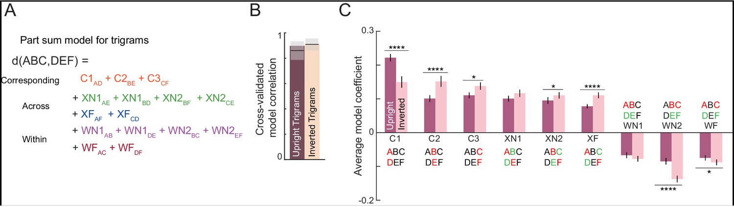
Part-sum model fits for upright and inverted trigrams.
(A) Schematic of part-sum model for trigrams. (B) Cross-validated model correlation of part-sum model for upright and inverted trigrams. (C) Average model coefficient (averaged across 6C2 = 15 terms) of each type for upright and inverted trigrams. Asterisks indicate statistical significance (* is p<0.05, ** is p<0.005, etc) calculated using a sign-rank test comparing the upright and inverted model terms. (D).
Appendix 6—figure 1
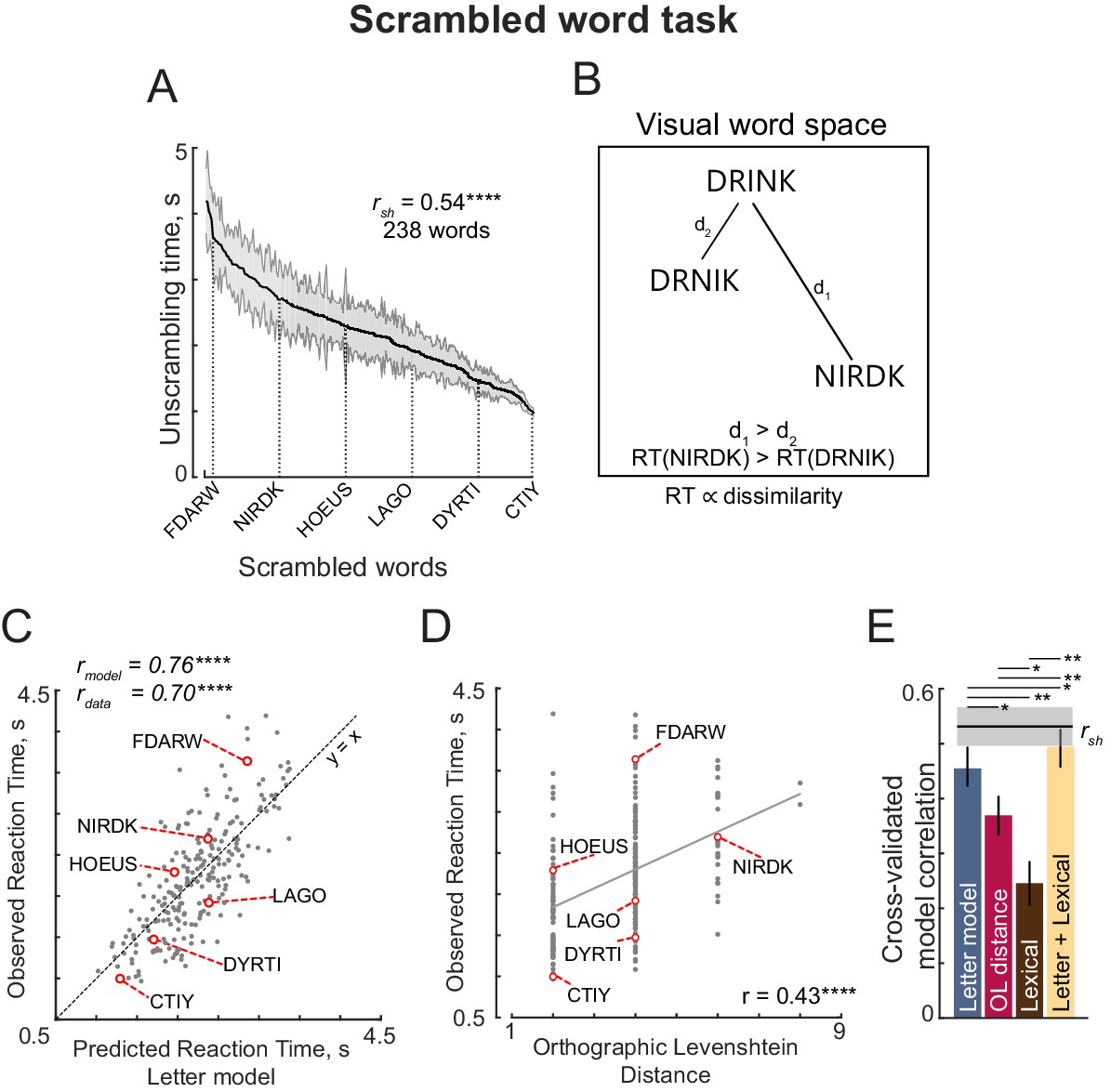
Jumbled word task (Experiment S7).
(A) Response times in the jumbled word task sorted in descending order. Shaded error bars represent s.e.m. Some example words are indicated using dotted lines. The split-half correlation between subjects (rsh) is indicated on the top left. (B) Schematic of visual word space, with one stored word (DRINK) and two jumbled versions (DRNIK and NIRDK). We predicted that the time taken by subjects to unscramble a jumbled word would be proportional to its dissimilarity to the stored word. Thus, subjects would take longer to unscramble NIRDK compared to DRINK. (C) Observed response times in the jumbled word task plotted against predictions from the letter model based on single letters with spatial summation. Each point represents one word. Asterisks indicate statistical significance (**** is p<0.00005). (D) Observed response times in the jumbled word task plotted against Orthographic Levenshtein (OL) distance. Each point represents one word. Asterisks indicate statistical significance (**** is p<0.00005). (E) Cross-validated model correlations for the letter model, OLD model, lexical model and the neural+lexical model. Model correlations were obtained by training each model on one half of subjects, and evaluating the correlation on the other half (error bars represent standard deviation across 1000 random splits). The upper bound on model fits is the split-half correlation (rsh), shown in black with shaded error bars representing standard deviation across the same random splits. All correlations were individually statistically significant (p<0.00005). Horizontal lines above shaded error bar depicts significant difference across different models that is the fraction of splits in which the observed difference was violated. All significant comparisons are indicated.
Appendix 7—figure 1
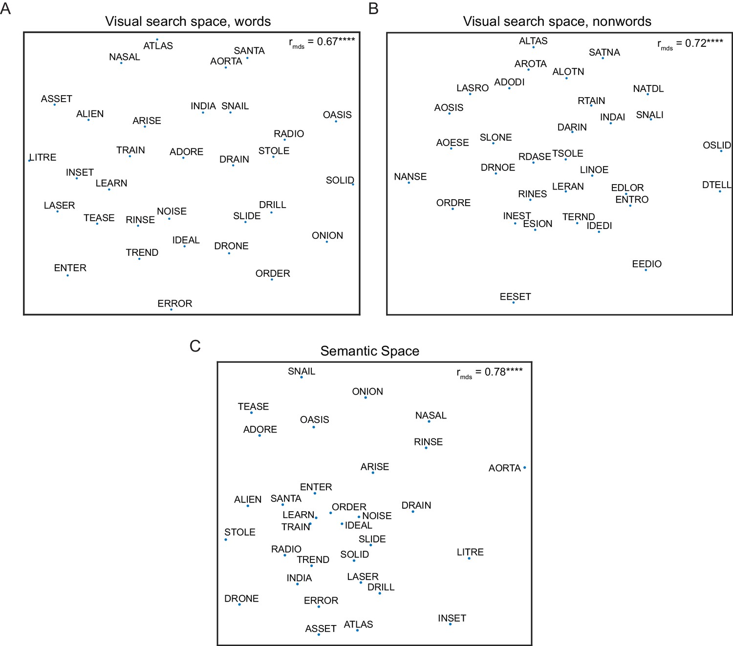
Multi-dimensional representation of words and nonwords.
(A) Perceptual space for words. we used multidimensional scaling to find the 2D coordinates of all words that best match the observed distances. In the resulting plot, nearby words indicate hard searches. The correlation coefficient between dissimilarities in 2D plane and the observed data is shown. Asterisks indicate significant correlation (**** is p<0.00005). (B) Same as (A) but for nonwords. (C) Same as (A) but for semantic space of words.
Appendix 7—figure 2
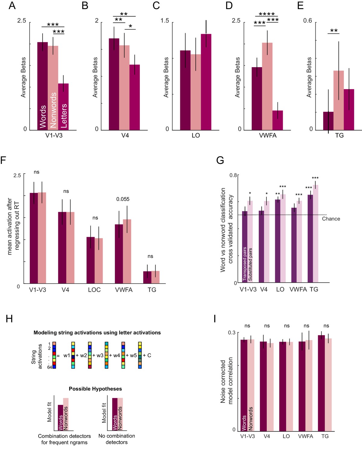
Neural activity.
(A) Average activation levels for words, nonwords, and letters. Error bar indicate ±1 s.e.m. across subjects. Asterisks indicate statistical significance (* is p<0.05, ** is p<0.005, etc. in a sign-rank test comparing subject-wise average activations). (B)-(E). Same as in A but for V4, Lateral Occipital areas, Visual Word Form Area, and Temporal Gyri respectively. (F) Mean activation level after regressing out the reaction time in the lexical decision task. Error bars indicate ±1 s.e.m. across subjects. (G) Cross-validated classification accuracy for transposed word-nonword pairs (dark) and substituted word-nonword pairs (light). Error bars indicate s.e.m. across subjects. Asterisks indicate statistical significance (* is p<0.05, ** is p<0.005, etc. in a sign-rank test comparing subject-wise accuracy w.r.t. chance level). (H) Schematic of the voxel model. The response of each voxel across strings is modeled as a linear combination of the constituent letter responses. Bottom: Hypothetical model fits based on the presence (right) or absence (left) of local combination detectors. Predicted responses for words will deviate from the observed responses under the influence of LCD. (I) Average model correlation (normalized using split-half correlation) for each ROI for words (dark) and nonwords (light). Error bar indicates s.e.m. across subject.
Appendix 7—figure 3
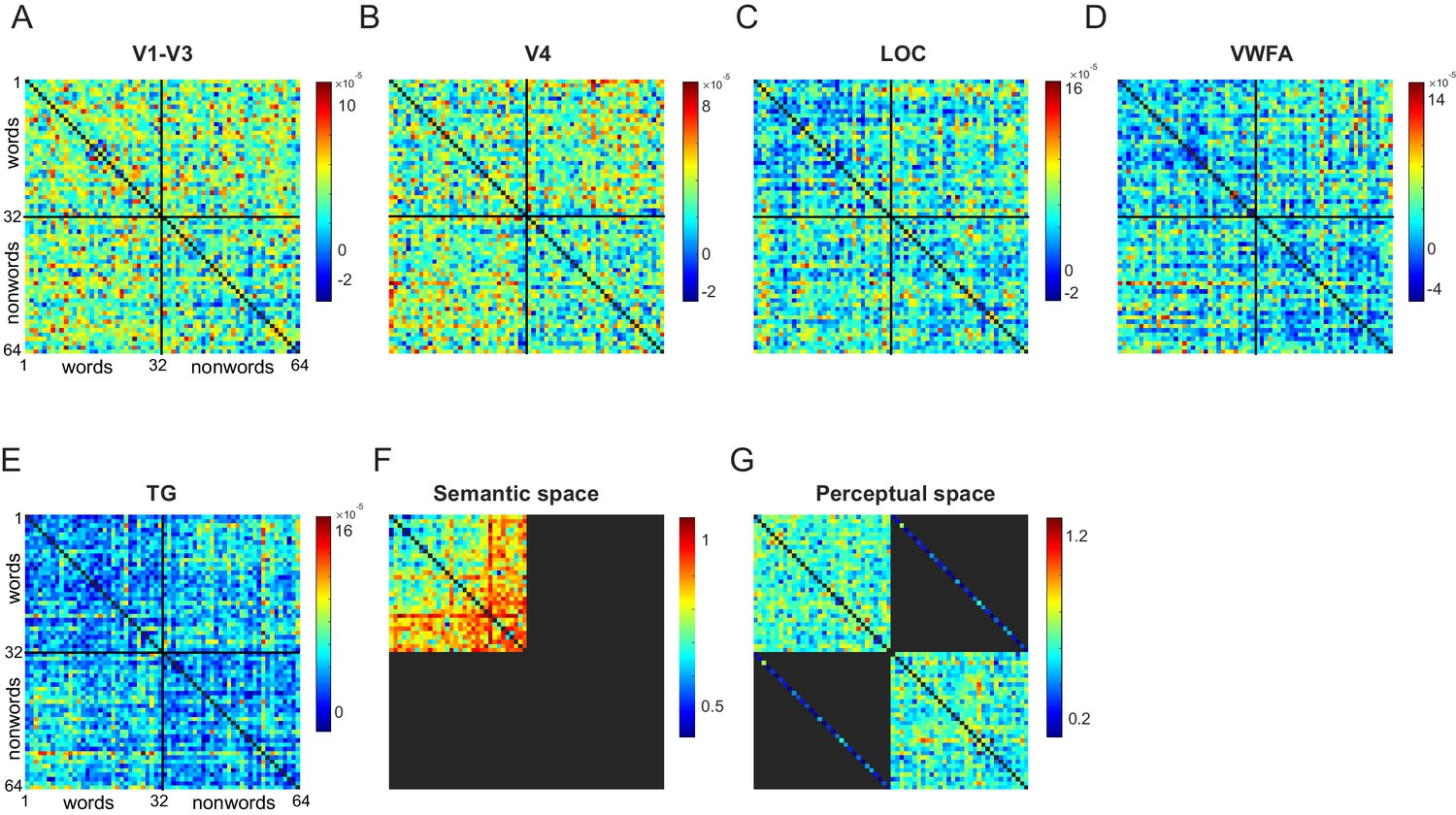
Representation dissimilarity matrix.
(A) Average pair-wise dissimilarity values for all possible pairs of words (1-32) and nonwords (33-64). Colour bar represents dissimilarity values that were estimated using a cross-validated, normalized variation of Mahalanobis distance. (B) - (E) Same as in A but for V4, Lateral Occipital areas, Visual Word Form Area, and Temporal Gyri respectively. (F) Pair-wise dissimilarity values in the semantic space across all possible pairs of words. Color bar represents dissimilarity values that is 1 – r (correlation between feature vectors for a given word pair) (G) Average pair-wise perceptual dissimilarities (1/search reaction time) for all possible pairs of words, nonwords, and corresponding word-nonword pairs.
Appendix 7—figure 4

Searchlight analysis.
(A) Searchlight map of correlation between neural activity and lexical decision time for each voxel. (B) Searchlight map of correlation between neural dissimilarity and search dissimilarities in behavior. (C) Searchlight map of correlation between neural dissimilarity and semantic dissimilarities. (D) Searchlight map depicting the difference in model fit for words versus nonwords for each voxel, averaged across subjects.
Appendix 7—figure 5
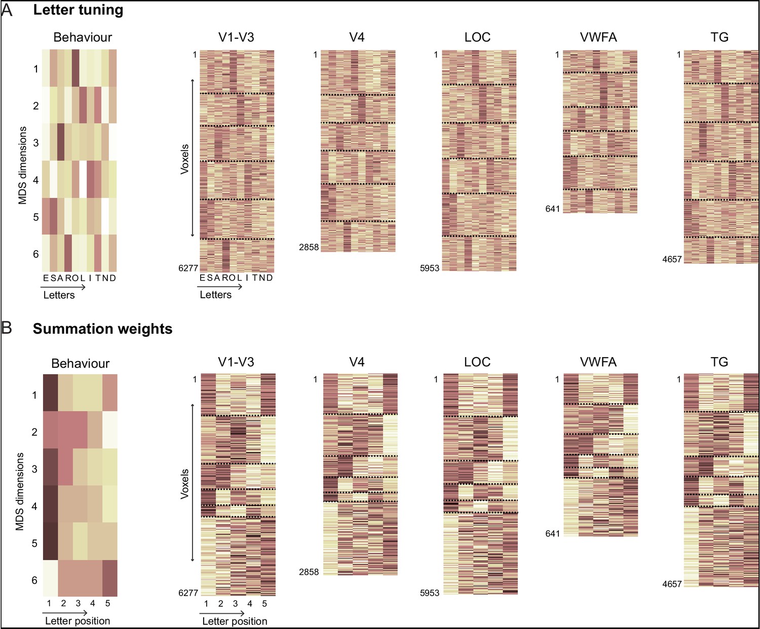
Comparison of letter tuning and summation weights.
(A) (Left) Response of 6 MDS neurons for all the 10 letters. (Right) Single letters response across all the voxels (concatenated across subjects) within a given ROI. Each voxels is sorted into one of six groups depending on which MDS neuron it matches best. The height of each ROI plot is logarithmically scaled to match the number of voxels across all subjects. Black dashed lines are used to separate the clusters corresponding to each MDS neuron. (B) Same as (A) but showing the summation weights corresponding to each MDS neuron or ROI voxel.
Tables
Table 1
Non-word stimuli in lexical decision task (Experiment 5).
| Variations of word ABCDE | four letter words | five letter words | six letter words | Total | |
|---|---|---|---|---|---|
| 1) | Edge transpositions: BACDE or ABCED | 15 | 15 | 20 | 50 |
| 2) | Middle transposition: ACBDE or ABDCE | 15 | 15 | 20 | 50 |
| 3) | Two-step edge transposition: CBADE or ABEDC | 0 | 20 | 30 | 50 |
| 4) | Two-step middle transposition: ADCBE | 0 | 20 | 30 | 50 |
| 5) | Random transposition: CDABE, ACDBE, etc. | 25 | 35 | 40 | 100 |
| 6) | Edge substitution: MZCDE or ABCMZ | 15 | 15 | 20 | 50 |
| 7) | Middle substitution: ABMZE | 15 | 15 | 20 | 50 |
| 8) | Random substitution and permutation: MACZE, AMDEZ, etc. | 15 | 15 | 20 | 50 |
| Total | 100 | 150 | 200 | 450 |
Appendix 4—table 1
Model fits for various choices of string alignment.
| Alignment | Letter model correlation | |||
|---|---|---|---|---|
| six vs five letter strings | six vs four-letter strings | five vs three-letter strings | four vs three-letter strings | |
| Left: ABCDEF vs EFGHxx | 0.54 | 0.66 | 0.58 | 0.57 |
| Right: ABCDEF vs xxEFGH | 0.51 | 0.66 | 0.57 | 0.58 |
| Centre: ABCDEF vs xEFGHx | - | 0.68 | 0.58 | - |
| Edge: ABCDEF vs EFxxGH | 0.55 | 0.63 | 0.60 | 0.59 |
Appendix 7—table 1
List of 32 words and 32 nonwords used in Experiment 6 & 7.
All words and nonwords were created from 10 single letters whose activations were also measured in the experiment.
| Middle Letter Transposition | Edge Letter Transposition | Middle Letter Substitution | Edge Letter Substitution | ||||
|---|---|---|---|---|---|---|---|
| Words | Nonwords | Words | Nonwords | Words | Nonwords | Words | Nonwords |
| AORTA | AROTA | STOLE | TSOLE | NOISE | NANSE | ONION | ESION |
| DRAIN | DARIN | OASIS | AOSIS | ERROR | EDLOR | RADIO | EEDIO |
| TREND | TERND | SOLID | OSLID | DRILL | DTELL | ASSET | EESET |
| ATLAS | ALTAS | TRAIN | RTAIN | ARISE | AOESE | TEASE | RDASE |
| DRONE | DRNOE | ORDER | ORDRE | LITRE | LINOE | ENTER | ENTRO |
| LEARN | LERAN | INDIA | INDAI | SLIDE | SLONE | IDEAL | IDEDI |
| SANTA | SATNA | RINSE | RINES | NASAL | NATDL | ADORE | ADODI |
| INSET | INEST | SNAIL | SNALI | ALIEN | ALOTN | LASER | LASRO |
Appendix 7—table 2
Variability in ROI definitions across subjects.
For each ROI we report the mean and standard deviation across subjects of the number of voxels, and the XYZ location of the voxel with peak T-value in the normalized brain.
| ROI | Definition | #voxels (mean ± sd) | ROI peak location |
|---|---|---|---|
| V1-V3 | Voxels activated forscrambled > fixation overlaid with anatomical mask of V1-V3 | 398 ± 131 | X: 8 ± 17 Y: -96 ± 5 Z: 6 ± 9 |
| V4 | Voxels activated forscrambled > fixation overlaid with anatomical mask of V4 | 185 ± 63 | X: 5 ± 26 Y: -88 ± 3 Z: 27 ± 11 |
| LO | Voxels activated for object > scrambled and not in other ROIs | 371 ± 115 | X: -17 ± 43 Y: -66 ± 15 Z: -19 ± 5 |
| VWFA | Voxels with known words > scrambled word in a contiguous region in fusiform gyrus | 52 ± 15 | X: -44 ± 4 Y: -50 ± 5 Z: -17 ± 5 |
| TG | Voxels with nativewords > scrambled word in a contiguous region in temporal gyrus | 289 ± 182 | X: -44 ± 39 Y: -43 ± 18 Z: 3 ± 9 |
Additional files
Download links
A two-part list of links to download the article, or parts of the article, in various formats.
Downloads (link to download the article as PDF)
Open citations (links to open the citations from this article in various online reference manager services)
Cite this article (links to download the citations from this article in formats compatible with various reference manager tools)
A compositional neural code in high-level visual cortex can explain jumbled word reading
eLife 9:e54846.
https://doi.org/10.7554/eLife.54846


