Differences in reward biased spatial representations in the lateral septum and hippocampus
- Department of Biology, MassachusettsInstitute of Technology, United States
- Picower Institute for Learning andMemory, Massachusetts Institute of Technology, United States
- Department of Brain and Cognitive Sciences, Massachusetts Institute of Technology, United States
Figures
Figure 1
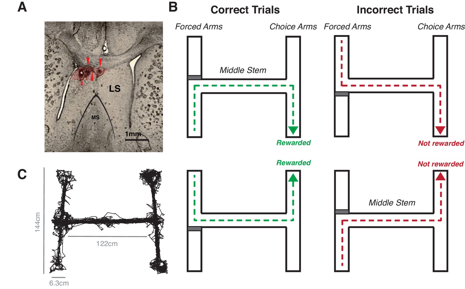
Rats were implanted with a tetrode array in the HPC and LS and run on a double sided T maze.
(A) Brain section from implanted rat, showing the lateral septum and electrolytic lesions made after recording. The red arrows mark lesions at the tetrode tips. Red shaded area indicates area where about 95% of lesions were seen. (B) Illustration of the maze task, which consisted of two phases: in the forced choice phase, animals were randomly forced with a block (represented by a red rectangle in a schematic) to either side of the T. In the free choice phase, animals had to choose, at the opposite end of the maze, the same side to which they were forced. If they made the correct choice, animals were rewarded with a sucrose and chocolate mixture. (C) Tracked position during one 30 min session.
Figure 2 with 1 supplement
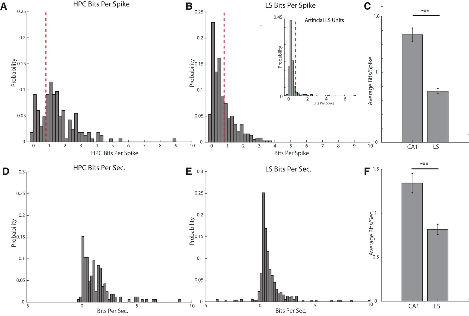
Hippocampal units have a higher average bits per spike and bits per second than septal units.
(A) Bits per spike of all recorded hippocampal units with an average spike rate >0.05 hz and full track coverage. A bits per spike cutoff of 0.8bits/spike is marked with a dotted line. (B) Larger graph: same as A for units in the lateral septum. Inset: bits per spike for artificially created LS units. The distribution of the bits/spike for the artificial units was highly significantly different than the distribution of bits/spike for actual units (KS test, p<10−15), and only 7.96% of artificial units had bits/spike measurements of greater than 0.8. The average bits/spike for the artificial units was 0.43, compared to an average value of 0.73 for actual units (two-tailed two sample t-test, t(818)=6.72, p<10−10). (C) Comparison of bits per spike for hippocampal and septal units. The average bits/spike of a CA1 cell is significantly higher than the average bits/spike of an LS cell. HPC mean 1.54+−1.2 bits/spike, LS mean 0.73+−0.7 bits/spike, two-tailed two sample t-test t(541)=9.42, p<0.001). Error bars represent standard error. (D) Bits per second of all recorded hippocampal units with an average spike rate >0.05 hz and full track coverage. (E) Same as D for units in the lateral septum. (F) Comparison of bits per second for hippocampal and septal units. CA1 units had a mean of 1.34+−1.4bits/sec, and LS cells had a mean 0.82+−1.1bits/sec. Units in the hippocampus had a significantly greater mean bits/sec than in the LS (two-tailed two sample t-test t(541)=4.57, p<0.001). Error bars represent standard error.
Figure 2—figure supplement 1
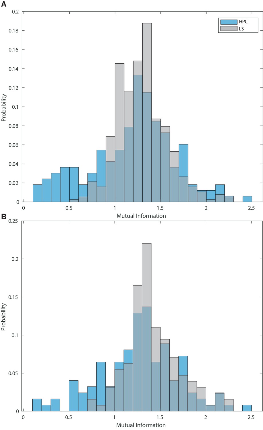
Mutual information in HPC and LS cells.
(A) Mutual information for all cells. Mean mutual information in the hippocampus is 1.20+−0.47, while mutual information in the septum is 1.29+−0.23. These values are significantly different (double sided t-test t(541)=-3.05, p<.005). Many LS cells without a place field may have a high mutual information score due to spatial correlations with speed and acceleration (Wirtshafter and Wilson, 2019). (B) Mutual information for cells with spikes/bit greater than or equal to 0.8. Mean mutual information for these cells in the hippocampus is 1.27+−0.44, while mutual information in the septum is 1.43+−0.30. These values are significantly different (double sided t-test t(249)=-3.35, p<.005).
Figure 3 with 2 supplements
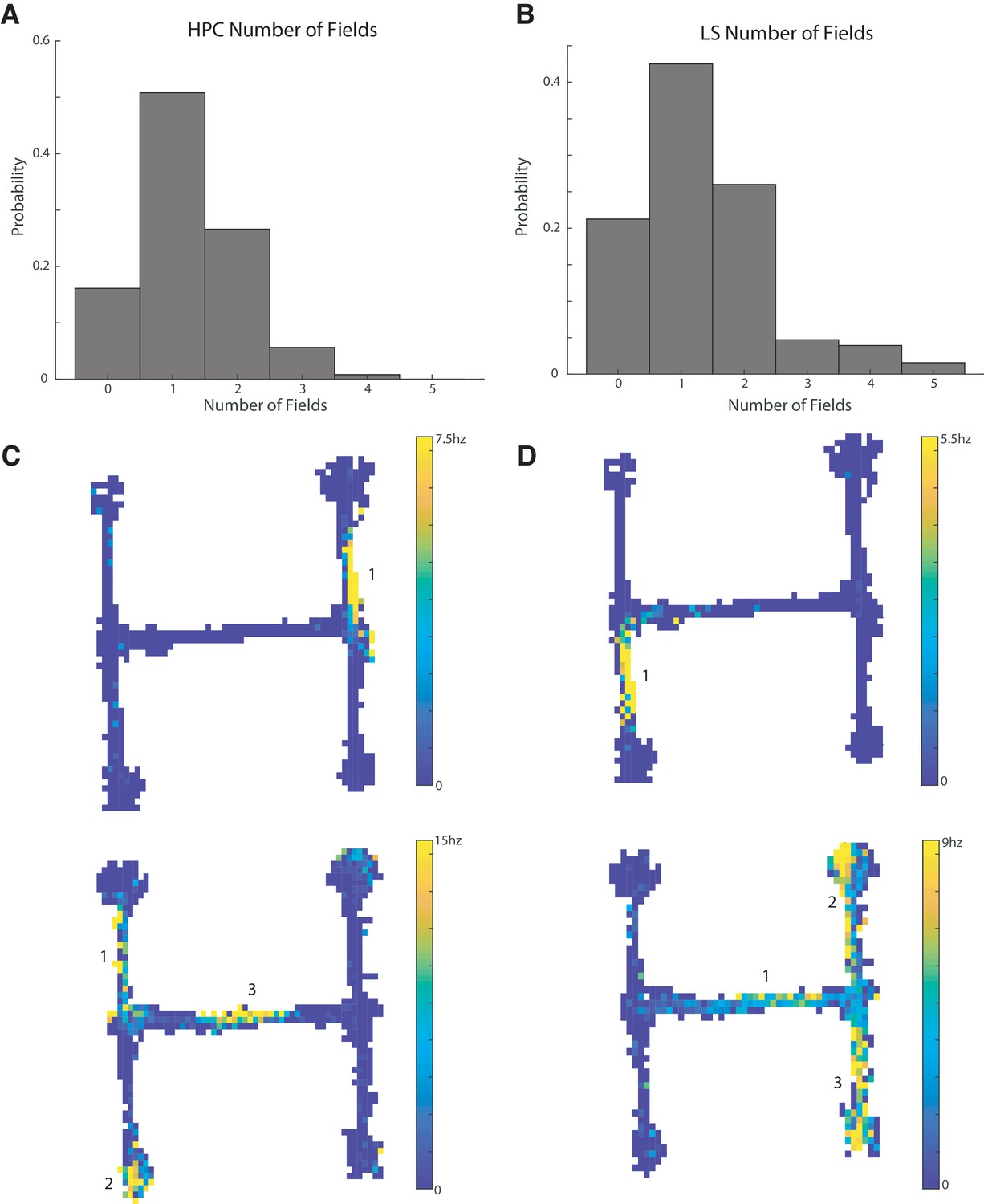
CA1 and LS place cells have a comparable number of place fields.
The distribution of field numbers was not significantly different between HPC and CA1 cells (two sample Kolmogorov-Smirnov (KS) test, p>0.5). (A) Number of fields in CA1 cells with a bits per spike greater than or equal to 0.8 bits/spike. (B) Same as A for lateral septum. (C) Example units in the CA1. Top: Example of a unit with a single place field. Bottom: example of a unit with three place fields. (D) Same as C but for the LS.
Figure 3—figure supplement 1
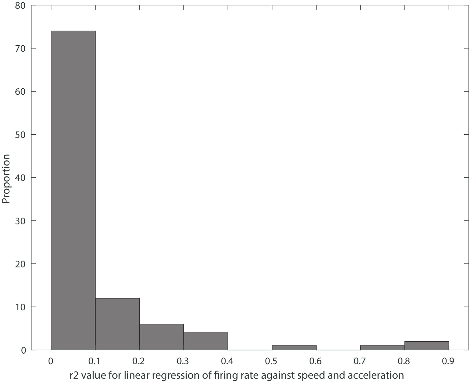
R2 values for linear regression of LS firing rate against speed and acceleration.
The median r2 value was 0.06.
Figure 3—figure supplement 2
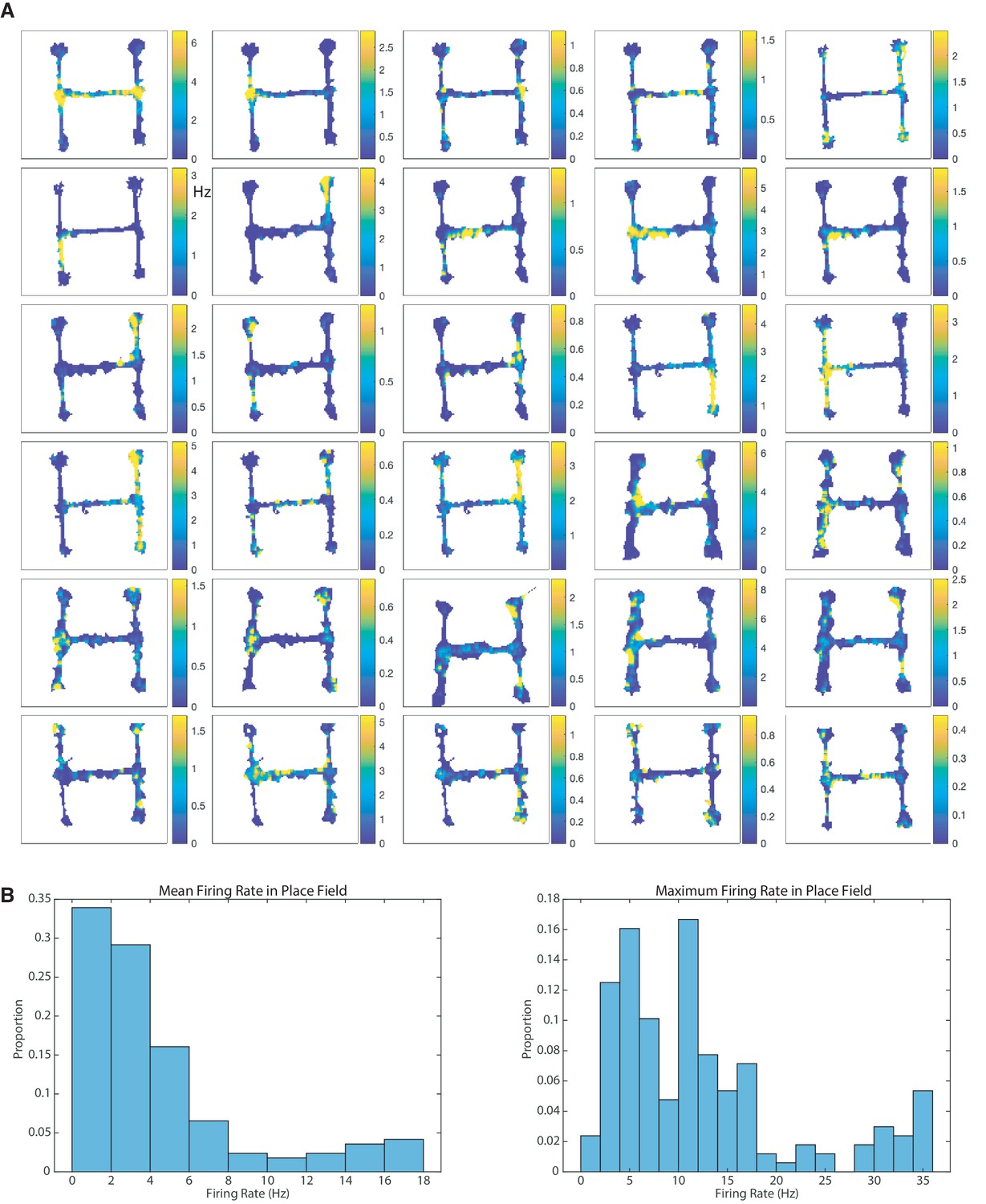
Place field representations and characteristics.
(A) Examples of spatial firing of 30 randomly selected LS cells. (B) Histograms of mean (left) and maximum (right) firing within a place field for all LS cells.
Figure 4
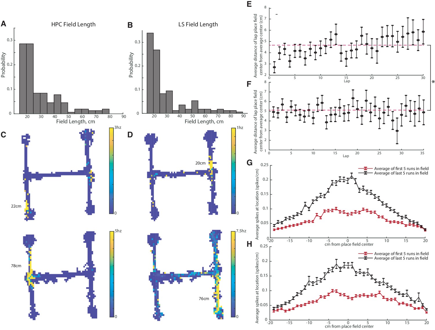
CA1 and LS place fields have comparable lengths and are modified with experience.
The average field lengths in CA and LS were not significantly different (two-tailed two sample t-test t(320)=-0.16, p>0.05). (A) Distribution of field lengths in the CA1. The average length of a CA1 place field was 29.1+-14.7cm. (B) Distribution of field lengths in the LS. The average length of an LS place field was 28.8+-16.6cm. (C) Example fields in the CA1. Top: example of a shorter field with a length of 22cm. Bottom: example of a longer field with a length of 78cm. (D) Example fields in the LS. Top: example of a shorter field with a length of 20cm. Bottom: example of a longer field with a length of 76cm. (E) Distance of highest HPC firing location from mean place field center during each lap. Average distance across all laps is marked with a dotted line The average distance from the field center in lap one is slightly but significantly different than the average field distance from the center in lap 30 (two-tailed two sample t-test t(177)=-2.7, p<0.01). (F) Distance of highest LS firing location from mean place field center during each lap. The average distance from the field center in lap one was not significantly different than the average field distance from the center in lap 30 (two-tailed two sample t-test t(207)=0.2, p>0.05). On average, compared to the LS, the HPC is slightly more accurate on the first lap as well as across all laps. (On the first lap, HPC has a mean distance of 2.7cm versus 4.9cm for the LS, two-tailed two sample t-test t(319)=-3.1, p<0.005. Across all laps, mean distance of 4.70cm for the HPC versus 5.12cm for the LS, two-tailed two sample t-test t(6792)=-2.5, p<0.05). (G) HPC spiking frequency per cm as a function of location around the place field center. The average spiking rate/cm of the first five runs through the field is marked in red, and the last five runs in black. Error bars represent standard error. The difference between the first and last run averages was significant for all cm values except +18cm and +20cm (all two-tailed two sample t-test). (H) Same as G but for the LS. The difference between the first and last run averages was significant for all cm values except -18cm (all two-tailed two sample t-test).
Figure 5 with 5 supplements

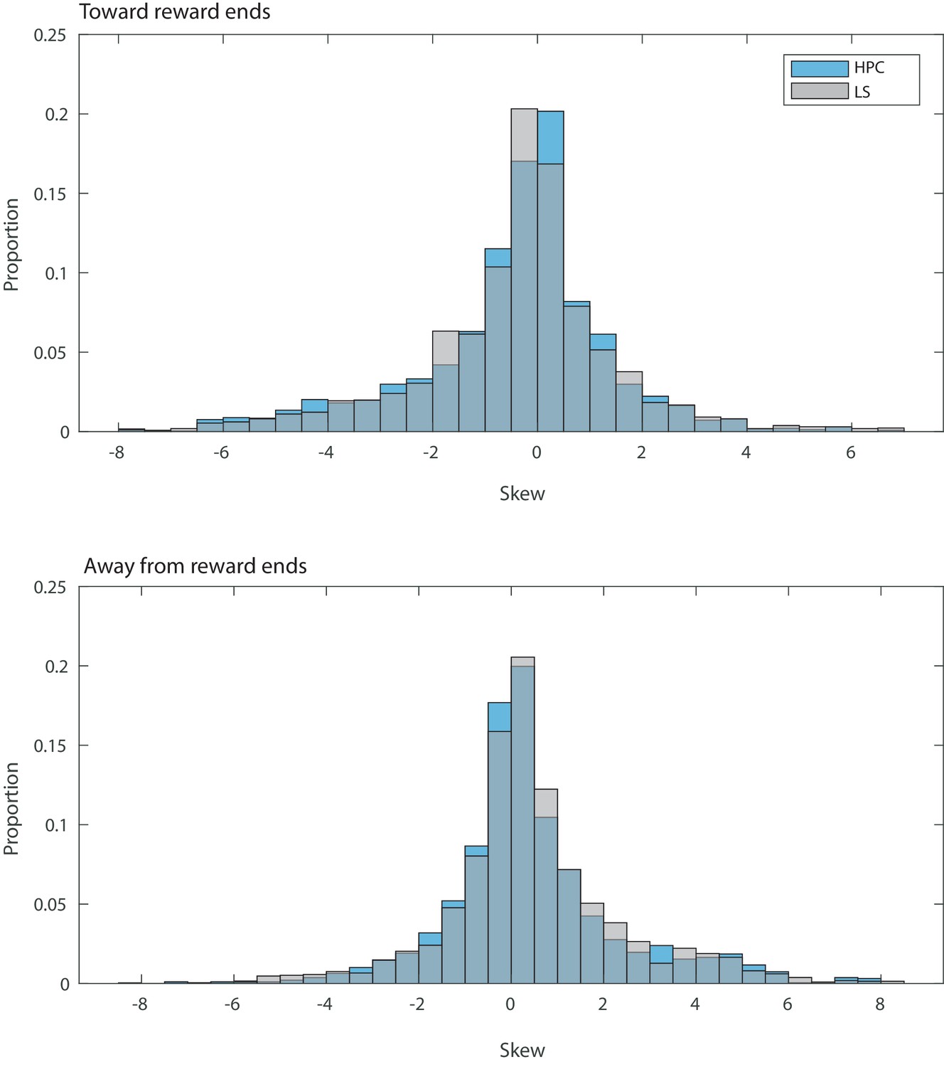
HPC and LS place cells have opposite directions of skew based on travel direction.
(A) Comparison of mean skew values within immediate reward proximity. Stars indicate significant differences between multiple populations. Plus signs indicate the mean is significantly different than 0. Xs indicate significant differences from a shuffled distribution, see Figure 5—figure supplement 3. Error bars represent standard error. In the hippocampus, there is a significant difference in mean skews based on direction of travel (two-tailed two sample t-test t(207)=-2.1, p<0.05). (B) Graph of distributions of skews in the hippocampus based on direction of travel. (C) Graph of distributions of skews in the septum based on direction of travel. (D) Schematic showing arms of the maze examined during immediate reward proximity. Toward reward direction is marked with a blue arrow, away from reward with a red arrow. (E) Comparison of mean skew values within immediate reward proximity. Stars indicate significant differences between multiple populations. Plus signs indicate the mean is significantly different than 0. Xs indicate significant differences from a shuffled distribution, see Figure 5—figure supplement 3. Left: Error bars represent standard error. Skew values were not significantly different for hippocampus traveling to and from reward (two sample two sided t-test, t(74)=-0.59 p>0.05), but were significantly different for LS cells to and from reward (two sample two sided t-test, t(108)=-2.10, p<0.05). (Skew for HPC away from reward is significantly different from a shuffled sample, two sample two sided t-test, t(301)=-2.05, p<0.05. Skew for LS away from reward is significantly different from zero, one sample two sided t-test, t(58)=-2.0, p=0.05). Right: Schematic for clarification of skew relative to reward location for both directions of travel. Arrow represents direction of travel, ‘R’ represents reward location. Note that while HPC skew away from reward for reward proximal cells appears to have a different direction than for all HPC cells when traveling away from reward, the two means are not significantly different (two sample two sided t-test, t(131)=1.62, p>0.05).
Figure 5—figure supplement 1
Distribution of skew values for each pass through a field.
Figure 5—figure supplement 2
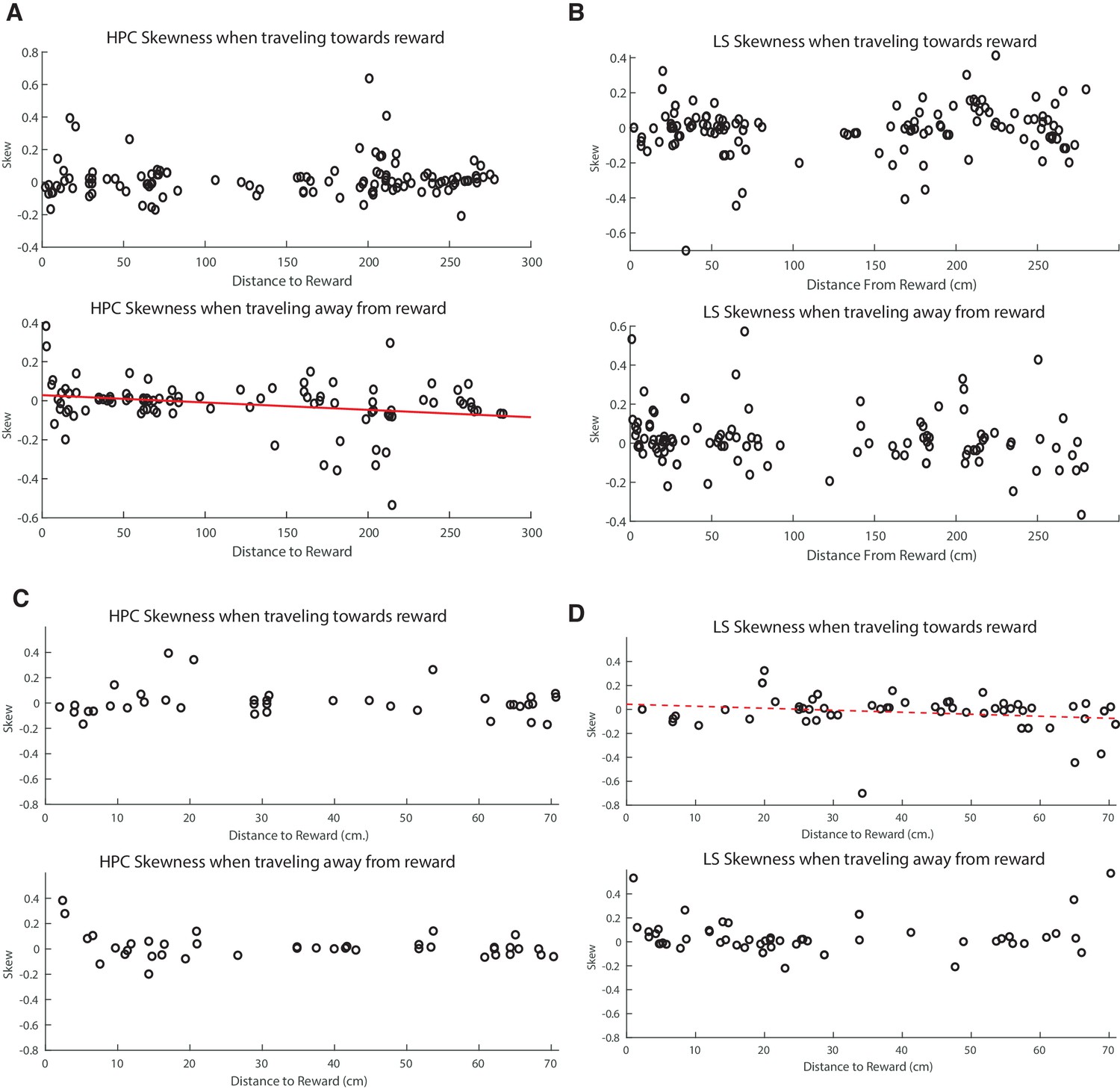
Skew versus distance to reward site across the whole track.
(A) Top: Scatter plot of skewness in HPC place cells versus distance to reward when traveling to reward. Bottom: Scatter plot of skewness in HPC place cells versus distance to reward when traveling away from reward. The linear correlation was significant (F statistic(1,92)=7.01, p<0.01, r2=0.07). (B) Same as A but in the LS. Neither linear correlation was significant (C) Same as A but only reward proximate HPC fields displayed. No significant linear correlations. (D) Same as B but only reward proximate LS fields displayed. Traveling to reward, the correlation neared significance (F statistic(1,60)=3.18, p=0.079, r2=0.03).
Figure 5—figure supplement 3
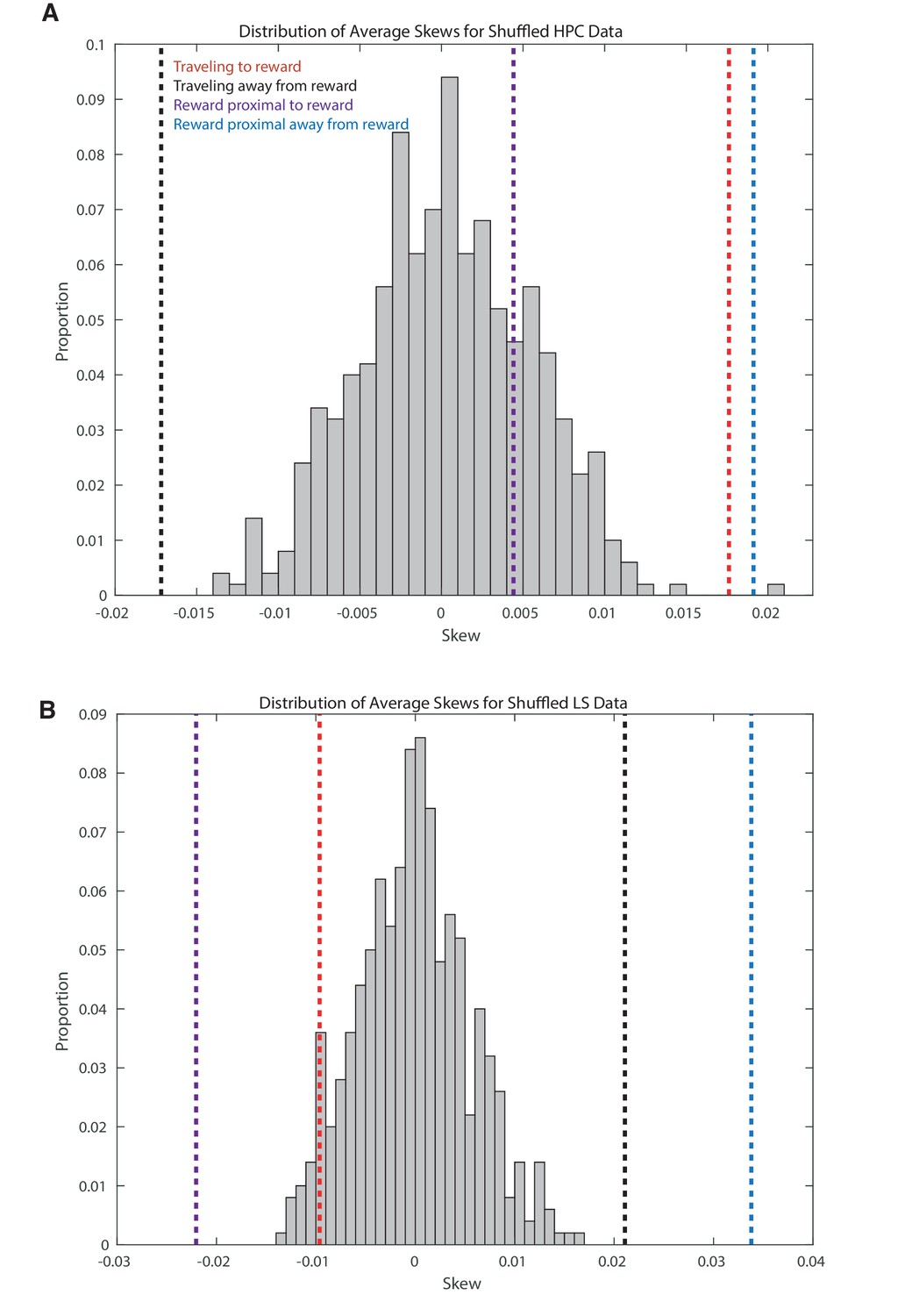
Distribution of skews for shuffled data.
(A) Distribution of skews for HPC shuffled data. A random distribution was obtained by shuffling firing rates within a firing field and then computing skew for the shuffled data. Average skew for 500 shuffled distributions were computed. The average skews for the actual data depicted in figure 5 are marked with dotted lines. (B) Same as A but for LS.
Figure 5—figure supplement 4

Skew is not impacted by uni- or bi- directional place fields.
(A) Comparison of average skew values for uni- and bi- directional LS place fields. There is no significant difference between the means directional (two-tailed two sample t-test, t(246)=-0.19, p=.85). (B) Comparison of average skew values for uni- and bi- directional LS place fields based on travel direction. There is no significant difference between the groups (one way anova, F(3,244) = 1.05, p>0.05). (C) Same as A but for HPC place fields. The mean skew was not significantly different between uni- and bi- directional place cells (two-tailed two sample t-test, t(207)=-0.59, p=0.55). (D) Same as B but for HPC place fields. There was no significant different between the groups (one way anova, F(3,205) = 0.29, p>0.05).
Figure 5—figure supplement 5
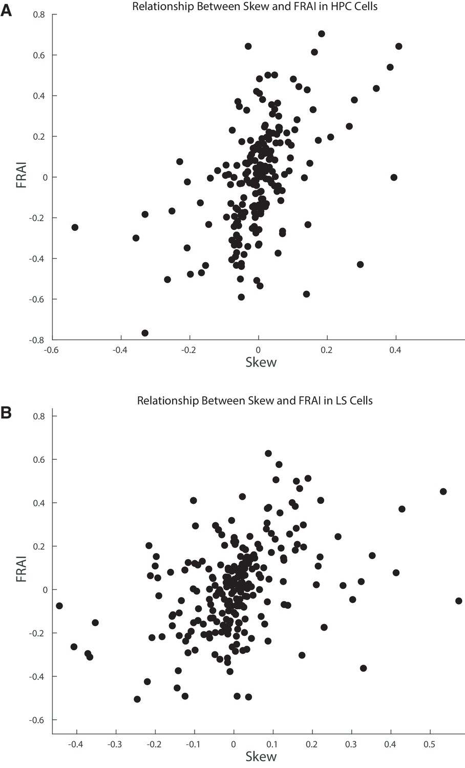
Skew and FRAI are highly linearly correlated in HPC and LS cells.
(A) There is a highly significant relationship between skew and FRAI in HPC cells (f(207)=61.0, p<9-13). (B) Same as A but in LS (F(247) = 43.77, p<9-10).
Figure 6 with 2 supplements
CA1 and LS fields have different location distributions, with LS place fields more biased toward reward locations.
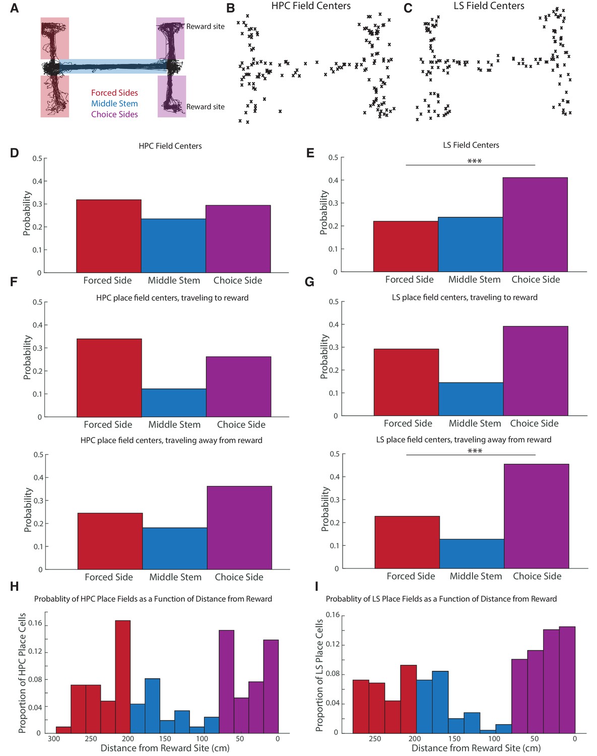
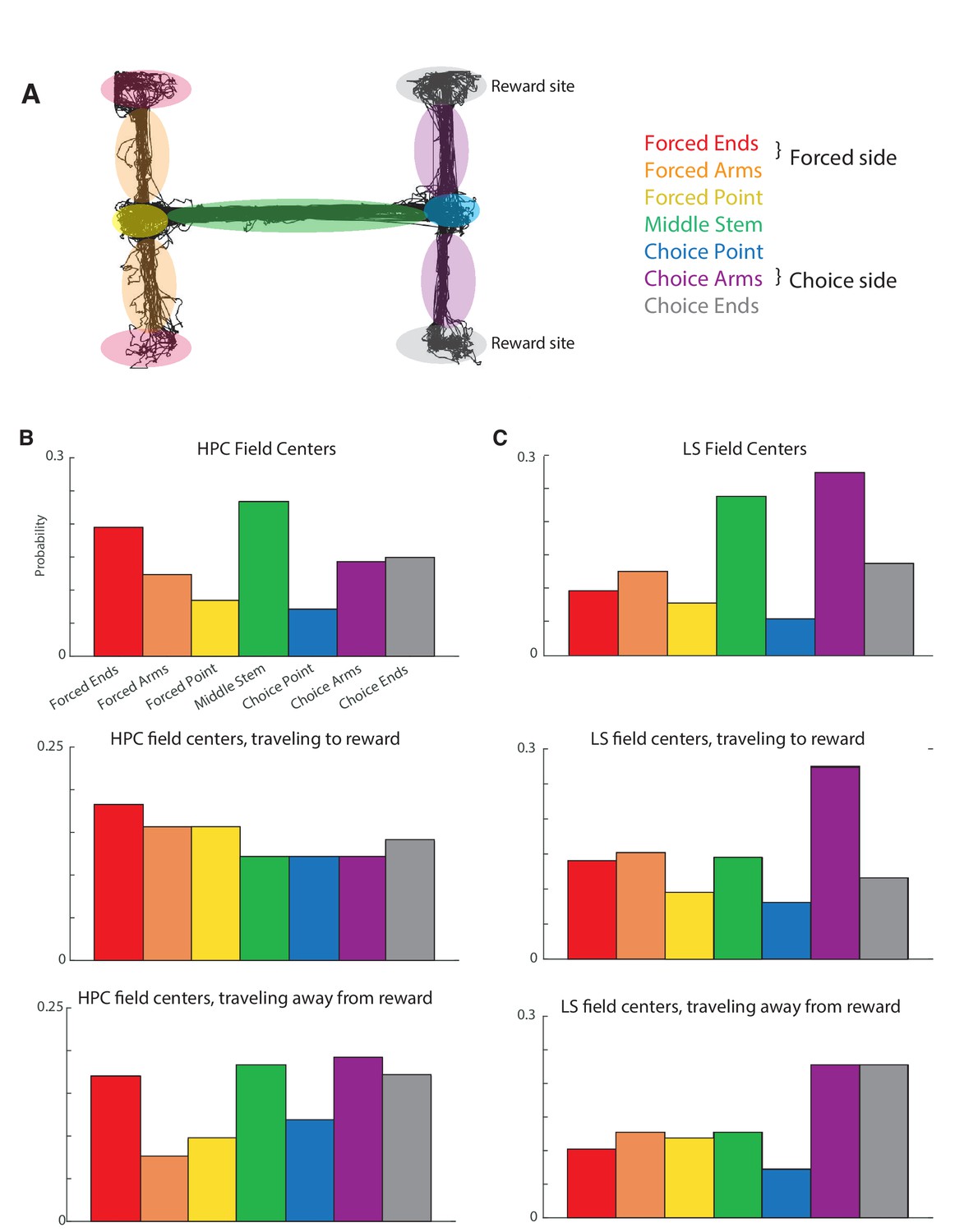
The distribution of place fields is significantly different between the hippocampus and the lateral septum (Pearson’s chi2 test, X2=12.7, p<0.05). (A) Schematic showing where the maze is split to identify place field location. (B) Scatter plot of HPC field centers (C) Scatter plot of LS field centers D. Distribution of HPC field centers. In CA1, place fields are no more likely to be on the choice side of the maze than the forced side (two-tailed two sample t-test t(364) = -2.34, p>0.05) (E) Distribution of LS field centers. There were significantly more fields in the choice arms compared to the forced arms (two-tailed two sample t-test t(334)=-3.8, p<0.001). The LS also has about 1.4 times, proportionally, more place fields in the choice side than the HPC does (41.1% of fields in the LS, versus 29.2% of fields in the HPC, two-tailed two sample t-test t(320) = -2.23, p<0.05). (F) Distribution of HPC place field centers by direction of travel. Top: traveling to reward. Bottom: traveling away from reward. (G) Distribution of HPC place field centers by direction of travel. Top: traveling to reward. Bottom: traveling away from reward. The LS had significantly more place fields on the choice side than the forced side in both travel directions, with the difference highly pronounced travelling away from reward (travelling toward reward two-tailed two sample t-test t(254)=1.82 p<0.10, travelling away from reward two-tailed two sample t-test t(218)=3.8 p<0.001). The distribution of place fields in the choice side was also significantly different based on the animal’s travel (one-tailed two sample t-test t(102)=-2.15, p<0.05). (H) The probability of finding a hippocampal place field as a function of distance from rewarded locations. As above, red represents the forced side of the maze, blue the middle arm, and purple the choice side. Note that the divisions between the three segments of the maze are not exactly represented in the histogram due to binning. (I) Same as H but for the LS.
Figure 6—figure supplement 1
Subdivided place field locations in HPC and LS.
(A) Schematic showing track divisions (B) Field locations in HPC. Top: for the full track, middle: traveling to reward, bottom: traveling away from reward. (C) Same, but for LS.
Figure 6—figure supplement 2
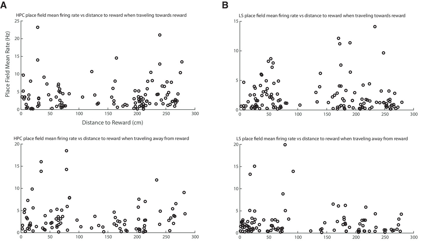
Mean place field firing rate is not correlated with distance to a reward site.
(A) Top: Scatter plot of mean firing rate in HPC place fields seen when the animal is traveling toward reward, plotted against distance to reward. Bottom: Scatter plot of mean firing rate in HPC place fields seen when the animal is traveling away from reward, plotted against distance to reward. (B) Same as A but in the LS.
Figure 7 with 3 supplements
Reward proximate LS cells are more synced with hippocampal activity than not proximate cells.
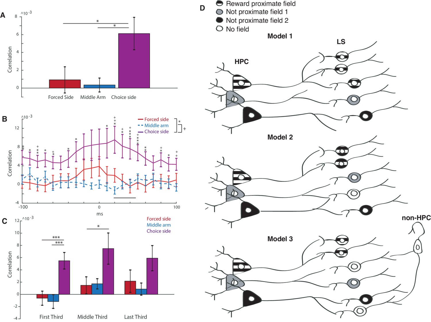
(A) Averaged cross correlation across a lag of −100 to 100 ms between coupled pairs of HPC and LS cells, based on place field location. Error bars show standard error. Forced side versus choice side: two-tailed two sample t-test t(67)=-2.2, p<0.05, middle arm versus choice side: two-tailed two sample t-test t(54)=-2.3, p<0.05). (B) Average of cross correlation traces at all lags between coupled pairs of HPC and LS cells, based on place field location. Error bars show standard error. Mean correlation peak for forced arm correlations was at 20 ms. Results from unpaired two tailed t-tests between forced and choice arms are indicated with stars: * indicates a p value of < 0.05 on an unpaired two tailed t-test, ** indicates a p value of < 0.01, and *** indicates a p value of < 0.005. Analogous results are shown between choice arm and middle arm using +. (C) Differences in cross correlations for HPC-LS pairs during the first, middle, and last third of a single trial. Error bars show standard error. * indicates a p value of < 0.05 on an unpaired two tailed t-test, *** indicates a p value of < 0.005. (D) Three models of LS innervation by HPC that may explain the overrepresentation of LS place fields by rewarded locations. Top: model 1. HPC cells with reward-proximate place fields selectively innervate more LS place cells. Middle: model 2. HPC cells with reward proximate place fields, and cells with other fields innervate the same number of LS cells. Hippocampal cells with non-proximate fields innervate overlapping cells, causing interference and resulting in fewer place fields in the LS that are not reward proximate. Bottom: model 3. HPC cells with reward proximate place fields, and cells with other fields innervate the same number of LS cells. Hippocampal cells with non-proximate fields innervate cells that are also innervated by other inputs, causing interference and resulting in fewer place fields in the LS that are not reward proximate.
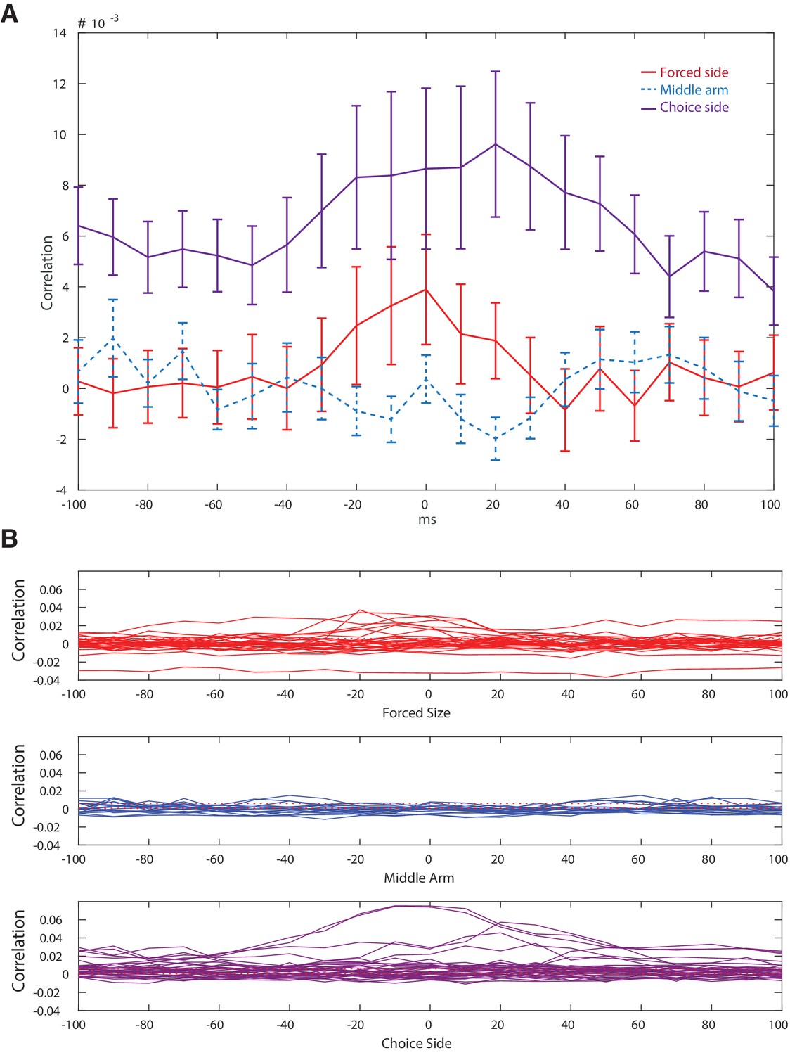
Figure 7—figure supplement 1

Cross correlation between all coupled pairs of HPC and LS cells, based on place field location.
Cross correlation is across a lag of -100 to 100ms. (A) Top panel: correlations between firing of cells with place fields on the forced side of the maze. Upper black bar represents average peak correlation for cells with fields on the choice size. Lower black bar(s) (too close together to be separate) represent average peak cross correlation for place fields in the forced and middle arms. Middle: Same as top but for cells with fields in the middle arm. Bottom: Same but for cells with fields on the choice size. (B) Same as A but for shuffled spike trains. We shuffled the spike trains of all the HPC and LS pairs on the forced arm and found an average correlation of 7.71e-05, with a 95% confidence interval of [-8.89e-05, 2.43e04]. Out of 36 unit pairs on the forced arm, the average of 26 of these pairs (72%) fell above the 95% confidence interval for shuffled data.
Figure 7—figure supplement 2
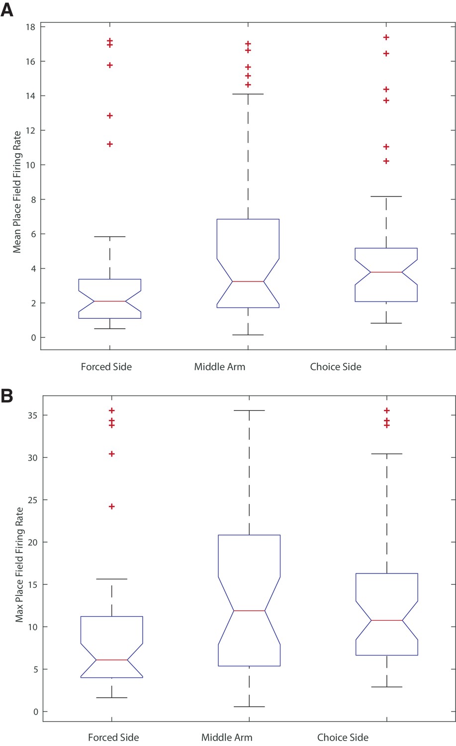
Mean and maximum within-field firing rates for LS place cells based on location.
(A) Mean within field firing rates for LS cells with place fields on the forced side, middle arm, and choice side. The means of three distributions were not significantly different (One way anova, F(2,112) = 1.15, p>0.05). (B) Mean within field firing rates for LS cells with place fields on the forced side, middle arm, and choice side. The means of the three distributions were not significantly different (One way anova, F(2,112) = 1.93, p>0.05).
Figure 7—figure supplement 3
Differences in cross correlations are not due to differences HPC-LS place field pair proximity in the different maze arms.
We sought to ensure that the higher cross correlation values were not the result of more place fields in the choice arm resulting in a lower average difference between field centers of HPC-LS matched pairs. We first decided to determine if there was a difference in the average distance between LS and HPC place field pairs for the forced side, central stem, and choice side. We found that there was no significant difference between the average distance between LS and HPC pairs in the forced arm versus choice arm (two-tailed two sample t-test, t(67) = 1.8, p>0.05), so the proximity of HPC-LS pairs did not account for the difference in cross correlation values for forced vs. choice sides. There was a small (3cm) but significant (two-tailed two sample t-test, t(51) = 2.2, p=0.03) difference in distances when comparing the choice side to the middle stem. (Running a one way anova with all three values, F(3,83) = 3.24, p = 0.04). To further ensure that distance between pair centers was not causing the increase cross correlation in the choice arm, we subsampled the data. We found that eliminating the very closest pairs (pairs that had centers within 3cm of each other) was more than sufficient to result in an insignificant difference between forced, choice, and middle pair distances (one way anova F(3,84) = 1.92, p>0.05, with both t-tests also p>0.05). When subsampled as described, the average cross correlation for pairs on the choice side was still significantly higher than the average in either the forced side or middle stem (double sided t tests, t(51) = 1.96 p<0.05 for comparing forced to choice and t(51) = 2.2 p<0.05 for comparing central to choice). (A) The average cross correlations of subsampled data. (B) All cross correlations of subsampled data.
Additional files
Download links
A two-part list of links to download the article, or parts of the article, in various formats.
Downloads (link to download the article as PDF)
Open citations (links to open the citations from this article in various online reference manager services)
Cite this article (links to download the citations from this article in formats compatible with various reference manager tools)
Differences in reward biased spatial representations in the lateral septum and hippocampus
eLife 9:e55252.
https://doi.org/10.7554/eLife.55252


