Differentiating between integration and non-integration strategies in perceptual decision making
- Department of Neuroscience, Columbia University, United States
- Mortimer B. Zuckerman Mind Brain Behavior Institute and The Kavli Institute for Brain Science, Columbia University, United States
- Department of Brain and Cognitive Sciences, University of Rochester, United States
- Center for Neuroscience and Department of Neurobiology, Physiology & Behavior, University of California, United States
- Howard Hughes Medical Institute, Columbia University, United States
Figures
Figure 1
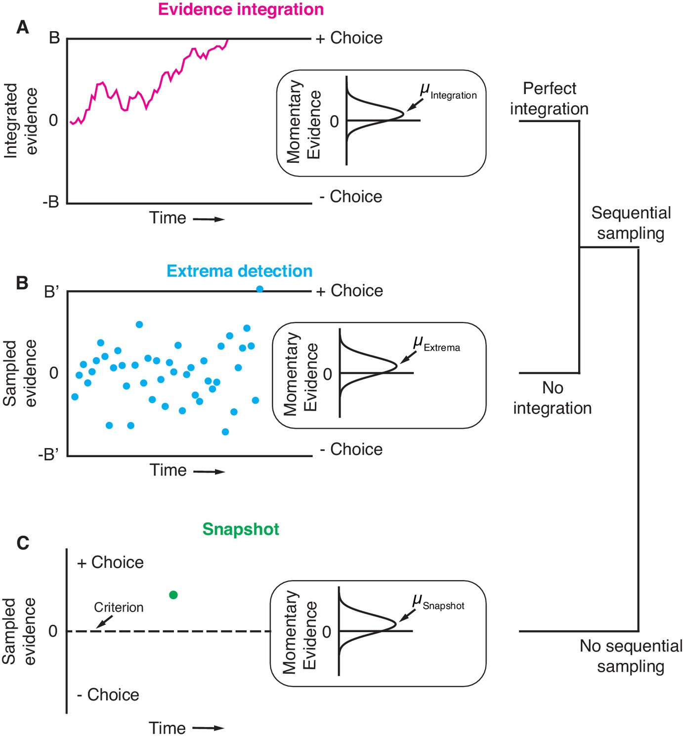
Three general decision-making models.
Each schematic represents the evidence that resulted in a single, positive choice. (A) The evidence integration model. Sequential samples of noisy momentary evidence are integrated over time until a decision-bound is reached, resulting in a positive or negative choice. The momentary evidence is assumed to be sampled from a Gaussian distribution with mean proportional to the stimulus strength. If the stimulus is extinguished before a decision-bound is reached, then the decision is based on the sign of the integrated evidence. (B) The extrema detection model. Momentary evidence is sequentially sampled but not integrated. A decision is made when one of the samples exceeds a detection threshold (i.e. an extremum is detected). Samples that do not exceed a detection threshold are ignored. If the stimulus is extinguished before an extremum is detected then the choice is determined randomly. (C) The snapshot model. Momentary evidence is neither sequentially sampled nor integrated. Instead, a single sample of evidence (i.e. a snapshot) is acquired on each trial and compared to a decision criterion to render a choice. The sampling time is random and determined before the trial begins.
Figure 2 with 1 supplement
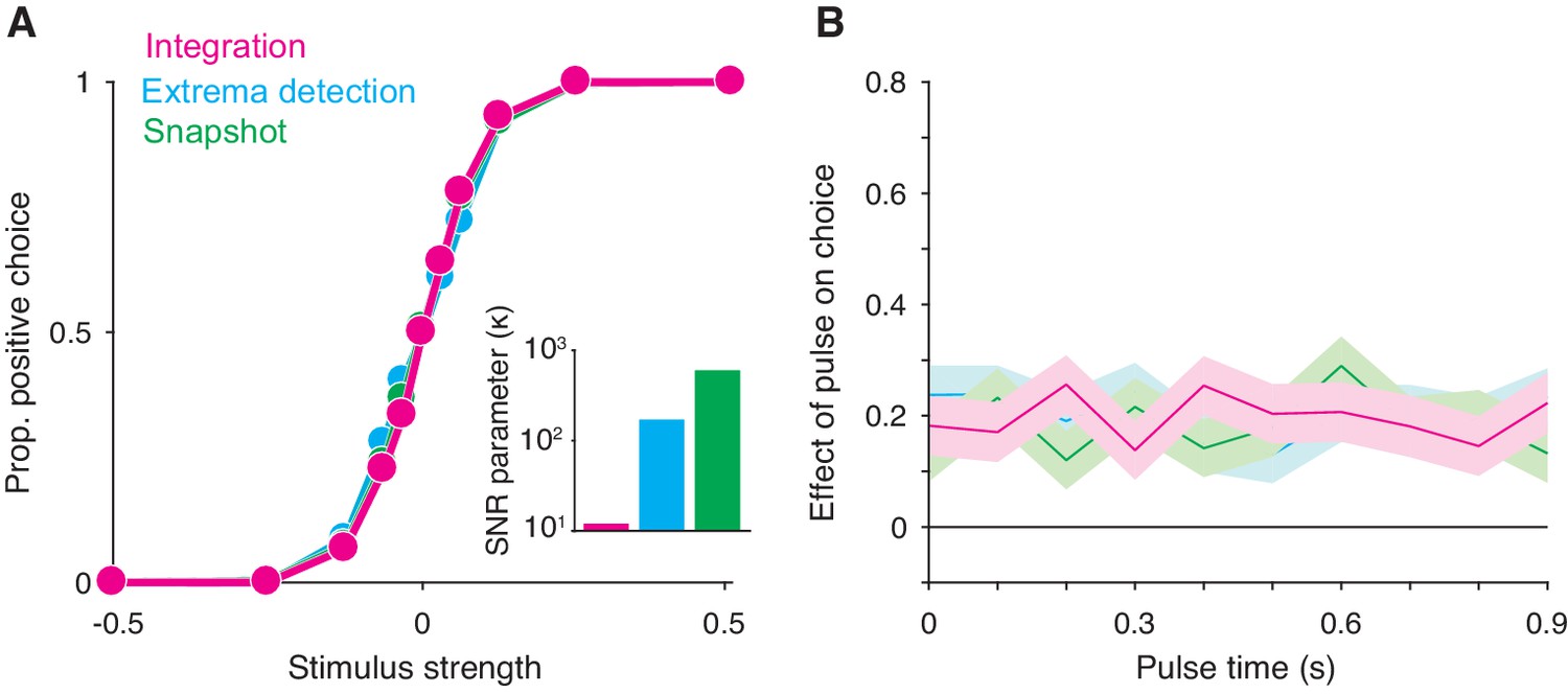
Integration and non-integration models produce similar psychometric functions and psychophysical kernels in a fixed stimulus duration task (stimulus duration = 1 second).
(A) Proportion of positive choices as a function of stimulus strength for each model simulation (N = 30,000 trials per simulation). The inset displays the SNR parameter () for each of the three models. All three models are capable of producing sigmoidal psychometric functions of similar slope but require different SNR parameters. (B) Psychophysical kernels produced from the choice-data in A. Each simulated trial contained a small, 100 ms long stimulus pulse that occurred at a pseudorandom time during the trial. Kernels are calculated by computing the pulse’s effect on choices (coefficients of a logistic regression, Equation 16) as a function of pulse time. Shaded region represents the standard error. Like integration, non-integration models are capable of producing equal temporal weighting throughout the stimulus presentation epoch.
Figure 2—figure supplement 1
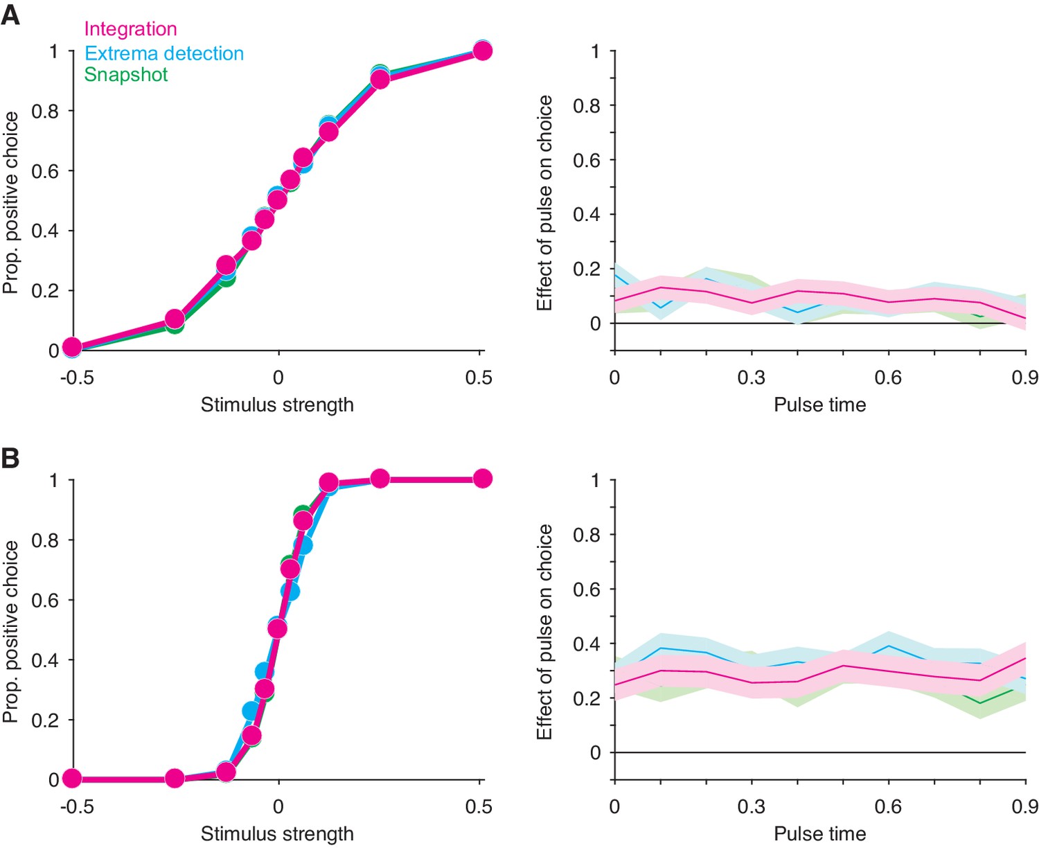
Extension of the exercise in Figure 2 to a low sensitivity regime (A) and a high sensitivity regime (B).
N = 30,000 trials per simulation.
Figure 3 with 1 supplement
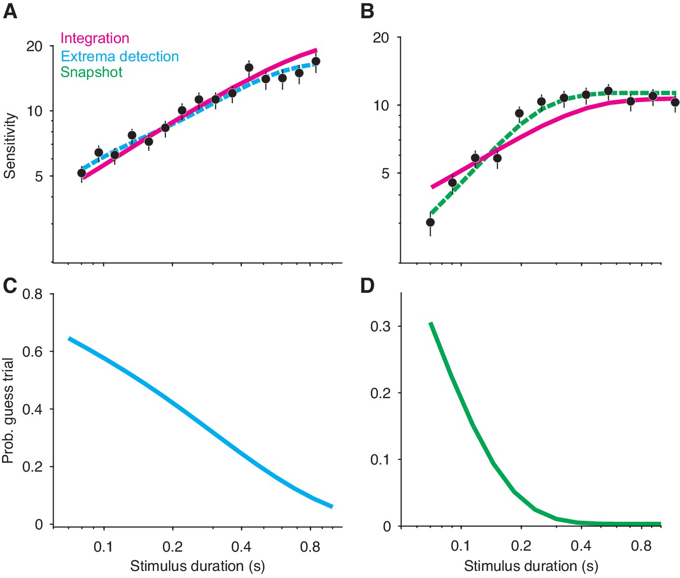
Non-integration models mimic integration in a variable stimulus duration (VSD) task.
(A) Sensitivity as a function of stimulus duration for simulated data generated from an extrema detection model (black data points; N = 20,000 total trials). Sensitivity is defined as the slope of a logistic function (Equation 18) fit to data from each stimulus duration (error bars are s.e.). The dashed cyan line represents the data-generating function (extrema detection). The solid magenta line represents the fit of the integration model to the simulated data. Although the data were generated by an extrema detection model, there is a close correspondence between the data and the integration fit. (B) The same as in (A), except the data were generated by a snapshot model. (C,D) The probability of a guess trial as a function of stimulus duration. Extrema detection (C) and snapshot (D) mimic integration in a VSD task in part because of the ‘guess’ rule. If the stimulus is extinguished before an extremum is detected or a snapshot is acquired, the choice is determined by a random guess.
Figure 3—figure supplement 1
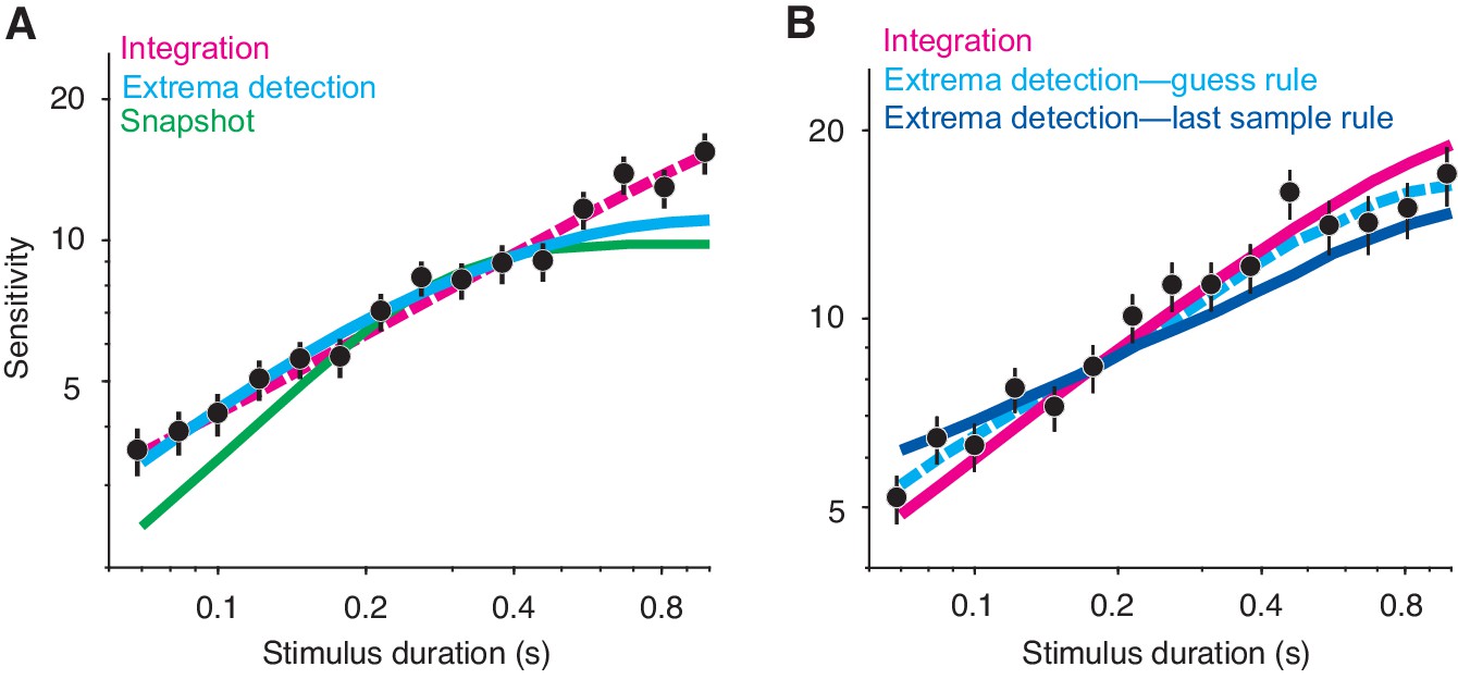
Integration as the data-generating model (A) and exploration of a last-sample rule in extrema detection (B).
(A) Extrema detection produces a reasonable fit (cyan curve) to simulated data generated by integration (black data points; N = 20,000 trials), although the fit underestimates sensitivity for the longest stimulus durations. The dashed magenta curve represents the data-generating function. The snapshot model (green curve) does not capture the main features of the simulated data. (B) A last-sample rule changes the behavior of the extrema detection model. The simulated data, integration model fit (magenta curve), and extrema detection model fit (with a guess rule; dashed cyan curve) are the same as in main Figure 3A. The dark blue curve represents the fit of an extrema detection model with a different ‘rule,’ in which the sign of the last sample of evidence determines the choice when the stimulus extinguishes before an extremum is detected. This model underestimates the slope of the sensitivity curve.
Figure 4 with 2 supplements
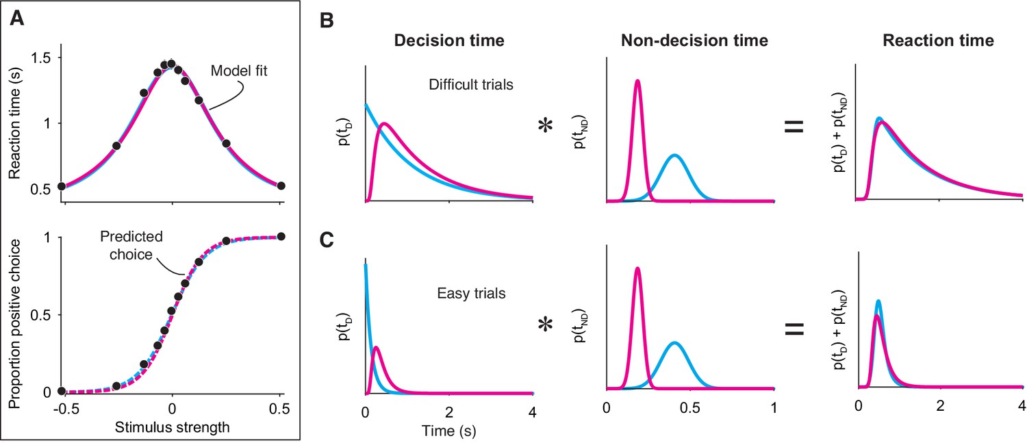
Integration and extrema detection behave similarly in free response tasks.
(A) Simulated choice-reaction time (RT) data generated by the extrema detection model (black data points; N = 19,800 total trials, 1800 trials per stimulus strength). RT (top) and the proportion of positive choices (bottom) are plotted as a function of stimulus strength. Solid colored curves are fits of the integration (magenta) and extrema detection (cyan) models to the mean RTs. Dashed curves are predictions using the parameters obtained from the RT fits. Note that the models’ predictions are indistinguishable. (B,C) The models produce similar RT distributions (right) but predict different decision times (left) and non-decision times (middle). The predicted RT distribution is the convolution (denoted by *) of the decision time distribution with the non-decision time distribution. (B) Depicts these distributions for difficult trials (stimulus strength = 0) and (C) depicts these for easy trials (stimulus strength = ±.512).
Figure 4—figure supplement 1
Extrema detection can fit RT means and predict choice-accuracy when integration serves as the data-generating model.
Black data points are simulations of an integration model (N = 20,000 total trials). Solid curves are fits of the integration (magenta) and extrema detection (cyan) models to mean RTs (top). Dashed curves (bottom) are the predictions of the models using the parameters obtained from the mean RT fits.
Figure 4—figure supplement 2
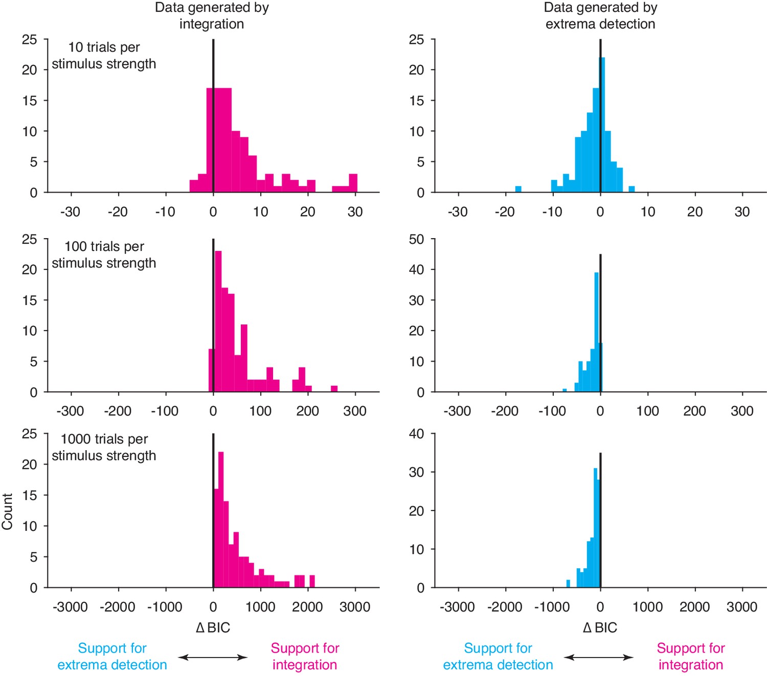
Model comparison between integration and extrema detection for simulated data.
We generated 600 datasets, half simulated from integration (left column) and half simulated from extrema detection (right column). We fit both models to each dataset and calculated the ∆BIC. Each row displays a different level of power, indicated by trials per stimulus strength. With 10 trials per stimulus strength, the majority of ∆BICs do not offer strong support for either model (|∆BIC| < 10 in 181 of 200 datasets). A large proportion of datasets with 100 trials per stimulus strength also do not yield strong support for either model (|∆BIC| < 10 in 63 out of 200 datasets). In contrast, all but one dataset with 1000 trials per stimulus strength yielded strong support for the data-generating model.
Figure 5
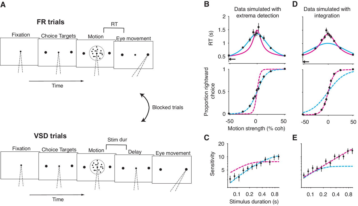
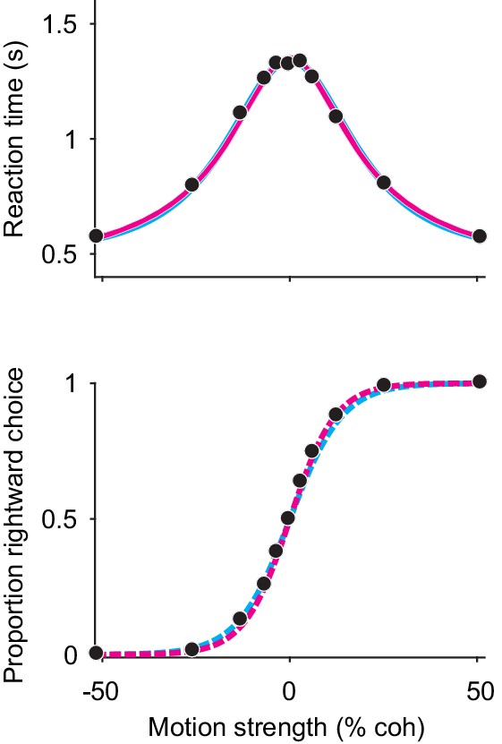
A motion discrimination task that disentangles the integration and extrema detection models.
(A) Schematic of the task. The task requires subjects to judge the direction (left versus right) of a random-dot-motion (RDM) movie in blocks of free response (FR) and variable stimulus duration (VSD) trials. In a second task (not shown), subjects were presented with 100% coherent motion only and were instructed to respond as fast as possible while maintaining perfect accuracy. (B) Simulation of FR trials in the RDM task (N = 2145 trials, 165 trials per stimulus strength). Reaction time (top) and the proportion of positive choices (bottom) are plotted as a function of stimulus strength. Data (black points) were generated from an extrema detection model (same parameters as in Figure 4). Positive (negative) motion coherence corresponds to rightward (leftward) motion. The arrow shows the non-decision time used to generate the simulated data. Solid curves are model fits to the mean RTs. Both models were constrained to use the data-generating non-decision time. Dashed curves are predictions using the parameters obtained from the RT fits. With the non-decision time constrained, only the data-generating model succeeds in fitting and predicting the data. (C) Simulation of VSD trials (N = 3000 trials). Data (black points) were generated with an extrema detection model, using the same κ parameter as in B. Dashed curves are model fits. Each model’s κ parameter was fixed to the value estimated from fits to the FR data. (D, E) Same as in (B) and (C) with integration as the data-generating model.
Figure 6 with 2 supplements

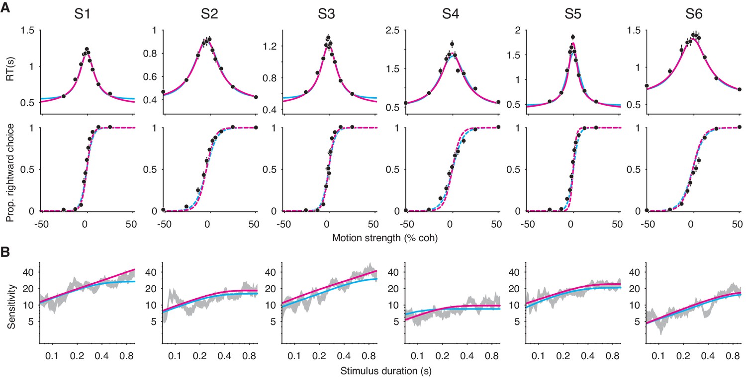
Failure of the extrema detection model and mixed success of the integration model in human subjects performing the RDM task.
(A) Free response (FR) trials. Reaction times (top) and proportion of rightward choices (bottom) as a function of motion strength for six human subjects (error bars are s.e.; ~1800 trials per subject). Positive (negative) motion coherence corresponds to rightward (leftward) motion. The arrows (top) indicate each subject’s estimated non-decision time from the speeded decision trials. Solid curves are model fits to the mean RTs (integration, magenta; extrema detection, cyan). Dashed curves are model predictions using the parameters obtained from the RT fits. Solid black lines (bottom) are fits of a logistic function to the choice-data alone. For visualization purposes, data from the interleaved 100% coherence trials are not shown (see Figure 6—figure supplement 1). (B) Variable stimulus duration (VSD) trials (~3000 trials per subject). Sensitivity as a function of stimulus duration for the same subjects as in (A). Sensitivity is estimated using logistic regression (sliding logarithmic time window, see Materials and methods). Dashed curves are model fits to the VSD data, using the κ parameter derived from model fits to the FR data.
-
Figure 6—source data 1
Data from the RDM task for each subject, separated by trial-type.
- https://cdn.elifesciences.org/articles/55365/elife-55365-fig6-data1-v2.zip
Figure 6—figure supplement 1
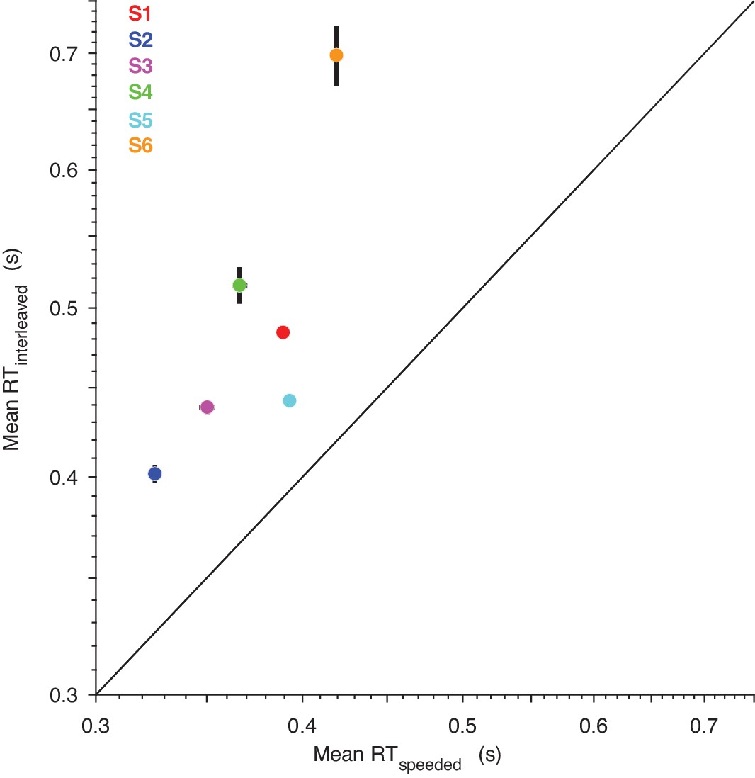
The reaction times from the ‘speeded decision’ experiment provide a better estimate of the non-decision time than those from the interleaved, 100% coherence trials.
The abscissa shows the estimated non-decision time from the speeded decisions, in which subjects were presented with 100% coherence trials only and were instructed to respond as fast as possible while maintaining perfect accuracy. The ordinate shows the mean RT on the 100% coherence trials that were interleaved in the main experiment. All subjects had perfect accuracy for both trial-types. Error bars are S.E.M.
Figure 6—figure supplement 2
Without constraints on the non-decision time and SNR, the models cannot be easily distinguished.
Data are the same as those in Figure 6. (A) FR trials. Sold curves are unconstrained fits of the integration (magenta) and extrema detection (cyan) models to mean RTs (top). The non-decision time was a free parameter and trials of 100% coherence were excluded. Dashed curves (bottom) are predictions generated from the parameters obtained from the mean RT fits. The quality of the fits and predictions are similar across both models. (B) VSD trials. Solid curves are model fits to subjects’ VSD data, allowing the K parameter to take on any value. Both models capture the main features of the data.
Figure 7 with 1 supplement
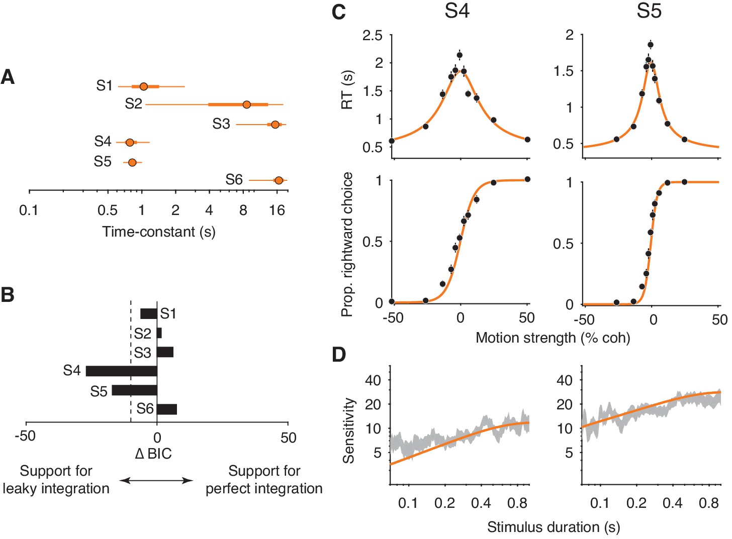
Fits of a leaky integration model.
(A) Integration time-constants estimated with a leaky integration model for each subject (S1–S6). The fits to FR and VSD data were constrained to share a common κ parameter. Thick and thin lines represent 50% and 95% Bayesian credible intervals, respectively, estimated by Variational Bayesian Monte Carlo (VBMC; Acerbi, 2018). (B) Comparison of the leaky integration and perfect integration models. Negative ∆BIC values indicate support for the leaky integration model. The leaky integration model is supported in S4 and S5 (; dashed line). (C) Leaky integration model fits for FR trials from S4 and S5. Data are the same as in Figure 6. (D) Leaky integration model fits for VSD trials from the same subjects as in (C).
Figure 7—figure supplement 1
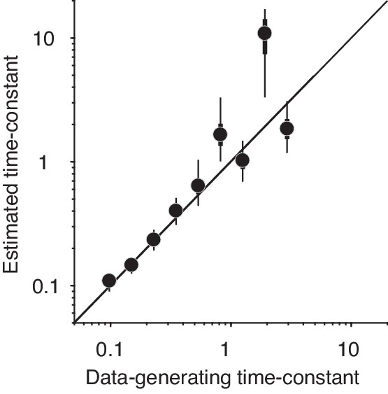
Parameter recovery for the leaky integration model.
We simulated the RDM task with a leaky integration model and produced nine datasets using different model parameters (Table 3). We fit these datasets with the leaky integration model and estimated the posterior distribution of the parameters with VBMC. The models were forced to use a common parameter for FR and VSD trials and to use the data-generating non-decision time parameters. The plot compares the estimated time-constant (median of the posterior) to the data-generating time-constant. Thick black lines are interquartile ranges and thin black lines are 95% credible intervals. The estimated time-constants from this fitting procedure closely matched the data-generating time-constant, especially when the data-generating time-constant was less than 1 second.
Author response image 1

Tables
Table 1
Parameters of the integration and extrema detection models (with flat bounds) fit to mean RT data.
∆BICs are relative to the fit of the integration model. Positive values indicate that integration produced a better fit/prediction.
| Model | Integration | Extrema detection | ||||||||||
|---|---|---|---|---|---|---|---|---|---|---|---|---|
| Subject | S1 | S2 | S3 | S4 | S5 | S6 | S1 | S2 | S3 | S4 | S5 | S6 |
| κ | 15.7 | 13.57 | 17.53 | 9.9 | 21.96 | 6.69 | 103.3 | 55.07 | 104.87 | 55.18 | 130.3 | 42.64 |
| B | 0.87 | 0.77 | 0.909 | 1.25 | 1.16 | 0.958 | 0.0757 | 0.0727 | 0.076 | 0.0786 | 0.078 | 0.0766 |
| C0 | −0.008 | −0.0453 | −0.012 | −0.006 | −0.005 | −0.02 | −0.006 | −0.0448 | −0.0121 | 0.026 | 0.001 | −0.031 |
| mean (empirical) | 0.39 | 0.326 | 0.394 | 0.367 | 0.351 | 0.42 | 0.39 | 0.326 | 0.394 | 0.367 | 0.351 | 0.42 |
| ∆BIC: RT fit | 0 | 0 | 0 | 0 | 0 | 0 | 471.36 | 204.4 | 202.88 | 135 | 494.7 | 71.74 |
| ∆BIC: choice prediction | 0 | 0 | 0 | 0 | 0 | 0 | 127.42 | 90.64 | 146.38 | −31.78 | −11.62 | 121.38 |
Table 2
Parameters of the integration and extrema detection models with collapsing decision-bounds (see Materials and methods) fit to full RT distributions.
∆BIC values are relative to the fit of the integration model. Positive values indicate that integration produced a better fit.
| Model | Integration | Extrema detection | ||||||||||
|---|---|---|---|---|---|---|---|---|---|---|---|---|
| Subject | S1 | S2 | S3 | S4 | S5 | S6 | S1 | S2 | S3 | S4 | S5 | S6 |
| κ | 19.79 | 11.86 | 21.91 | 7.97 | 19.11 | 5.88 | 120.2 | 60.84 | 170.91 | 55.38 | 146.52 | 36.26 |
| B0 | 1.0828 | 0.698 | 1.159 | 1.15 | 1.08 | 0.98 | 0.0765 | 0.0739 | 0.085 | 0.0796 | 0.0791 | 0.0772 |
| a | 0.7 | 5.0 | 0.53 | 14.3 | 5.24 | 1.97 | 47.34 | 1.2 | 0.165 | 0.285 | 0.55 | 9.18 |
| d | 0.4 | 8.0 | 0.33 | 12.4 | 12.36 | 31 | 2.3 | 4.0 | 0.0005 | 49 | 49 | 32 |
| (empirical) | 0.39 | 0.326 | 0.394 | 0.367 | 0.351 | 0.42 | 0.39 | 0.326 | 0.394 | 0.367 | 0.351 | 0.42 |
| (empirical) | 0.05 | 0.043 | 0.036 | 0.079 | 0.07 | 0.068 | 0.05 | 0.043 | 0.036 | 0.079 | 0.07 | 0.069 |
| C0 | −0.0103 | −0.05 | −0.0099 | −0.002 | −0.0054 | 0.0139 | −0.0126 | −0.0746 | −0.0107 | −0.0035 | −0.0064 | 0.017 |
| ∆BIC | 0 | 0 | 0 | 0 | 0 | 0 | 1,495.1 | 607.1 | 801.2 | 464.0 | 701.2 | 889.1 |
Table 3
Generating parameters used for the parameter recovery analysis (Figure 7—figure supplement 1).
Each row represents the set of three parameters used to simulate data with the leaky integration model.
| Model parameters | |||
|---|---|---|---|
| Simulation | κ | B | 𝜏 |
| 1 | 15 | 0.5 | 0.1 |
| 2 | 14.63 | 0.55 | 0.15 |
| 3 | 14.25 | 0.59 | 0.23 |
| 4 | 13.88 | 0.65 | 0.36 |
| 5 | 13.5 | 0.71 | 0.55 |
| 6 | 13.13 | 0.77 | 0.84 |
| 7 | 12.75 | 0.84 | 1.28 |
| 8 | 12.38 | 0.92 | 1.96 |
| 9 | 12 | 1 | 3 |
Additional files
Download links
A two-part list of links to download the article, or parts of the article, in various formats.
Downloads (link to download the article as PDF)
Open citations (links to open the citations from this article in various online reference manager services)
Cite this article (links to download the citations from this article in formats compatible with various reference manager tools)
Differentiating between integration and non-integration strategies in perceptual decision making
eLife 9:e55365.
https://doi.org/10.7554/eLife.55365


