A Bayesian and efficient observer model explains concurrent attractive and repulsive history biases in visual perception
- Donders Institute for Brain, Cognition and Behaviour, Radboud University, Netherlands
Figures
Figure 1
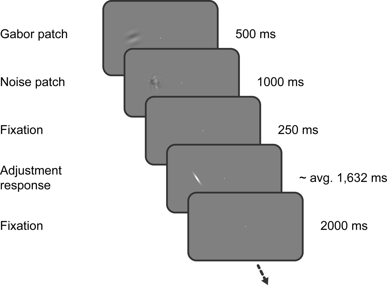
Task of Experiment 1.
Observers saw a Gabor stimulus followed by a noise mask and subsequently reproduced the orientation of the stimulus by adjusting a response bar. Stimulus presentation in the left or right visual field alternated between separate, interleaved blocks.
Figure 2
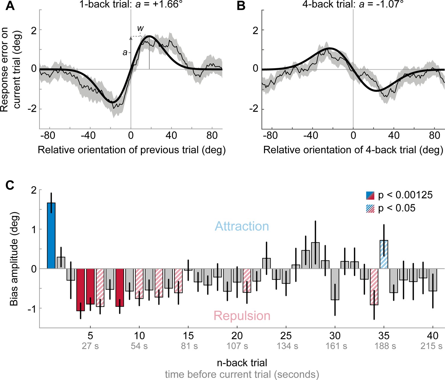
Results of Experiment 1: Estimation responses are attracted towards short-term, but repelled from long-term stimulus history.
(A) Serial dependence of current response errors on the previous stimulus orientation. We expressed the response errors (y-axis) as a function of the difference between previous and current stimulus orientation (x-axis). For positive x-values, the previous stimulus was oriented more clockwise than the current stimulus and for positive y-values the current response error was in the clockwise direction. Responses are systematically attracted towards the previous stimulus, as is revealed by the group moving average of response errors (thin black line). The attraction bias follows a Derivative-of-Gaussian shape (DoG, model fit shown as thick black line). Parameters a and w determine the height and width of the DoG curve, respectively. Parameter a was taken as the strength of serial dependence, as it indicates how much the response to the current stimulus orientation was biased towards or away from a previous stimulus with the maximally effective orientation difference between stimuli. Positive values for a mark an attractive bias. Shaded region depicts the SEM of the group moving average. (B) Current responses are systematically biased away from 4-back stimulus. (C) Attraction and repulsion biases exerted by the 40 preceding stimuli. Bias amplitudes show the amplitude parameter a of the DoG models, fit to the n-back conditioned response errors (see panel A and B). While the current response is attracted towards the 1-back stimulus, it is repelled from stimuli encountered further in the past. Colored bars indicate significant attraction (blue) and repulsion (red) biases (solid: Bonferroni correction for multiple comparisons; striped: no multiple comparison correction). Error bars represent 1 SD of the bootstrap distribution.
-
Figure 2—source data 1
Results of Experiment 1: Estimation responses are attracted towards short-term, but repelled from long-term stimulus history.
The source data file contains a csv file with the 1- to 40-back DoG model parameter estimates and a csv file with p-values for testing the model’s amplitude parameters against zero. It also contains csv files with moving averages of response errors conditioned on the 1- and 4-back trial, respectively (participants x orientation). Furthermore, it contains a mat file with all 1- to 40-back moving averages of each participant.
- https://cdn.elifesciences.org/articles/55389/elife-55389-fig2-data1-v2.zip
Figure 3
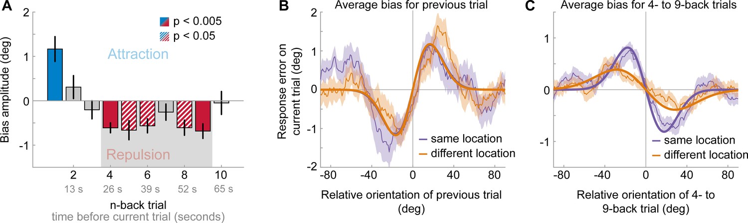
Results of Experiment 2: Long-term repulsive biases are spatially specific.
(A) Attraction and repulsion biases exerted by the 10 preceding stimuli, regardless of changes in spatial locations. The current response is attracted towards the previous stimulus, but repelled from stimuli seen 4 to 9 trials ago. Colored bars indicate significant attraction (blue) and repulsion (red) biases (solid: Bonferroni correction for multiple comparisons; striped: no multiple comparison correction). Error bars represent 1 SD of the bootstrap distribution. The gray shaded area marks the time window of interest for which we estimated the spatial specificity of the repulsive bias (panel C). (B) Serial dependence on previous stimulus, considering trials for which the previous stimulus was presented at the same location as the current stimulus (‘same location’, purple), or trials for which the previous and current stimulus location was 10 visual degrees apart (‘different location’, orange). Attractive serial dependence is similarly strong for same and different location trials. Shaded region depicts the SEM of the group moving average (thin lines). Thick lines show the best fitting DoG curves. Same data as shown in Experiment 1 by Fritsche et al., 2017. (C) Average serial dependence on 4- to 9-back stimuli for same (purple) or different (orange) location trials. Current responses are more strongly repelled from 4- to 9-back stimuli, when current and past stimuli were presented at the same spatial location.
-
Figure 3—source data 1
Results of Experiment 2: Long-term repulsive biases are spatially specific.
The source data file contains a csv file with the 1- to 10-back DoG model parameter estimates and a csv file with p-values for testing the model’s amplitude parameters against zero. It also contains two csv files with model parameters fit to 1-back or 4- to 9-back conditioned response errors, split by location change. Furthermore, it contains a mat file with all 1- to 10-back moving averages of each participant (same and different locations).
- https://cdn.elifesciences.org/articles/55389/elife-55389-fig3-data1-v2.zip
Figure 4

Results of Experiment 3: Long-term repulsive biases are not strongly modulated by working memory delay.
(A) Attraction and repulsion biases exerted by the 10 preceding stimuli, pooled across response delay conditions. The current response is attracted towards the previous stimulus, but repelled from stimuli seen 2 to 6 trials ago. Colored bars indicate significant attraction (blue) and repulsion (red) biases (solid: Bonferroni correction for multiple comparisons; striped: no multiple comparison correction). Error bars represent 1 SD of the bootstrap distribution. The gray shaded area marks the time window of interest for which we estimated the working memory delay dependence of the repulsive bias (panel C). (B) Serial dependence on previous stimulus, considering trials for which the delay between current stimulus and response was short (green) or long (pink). Attractive serial dependence increases with working memory delay on the current trial. Shaded region depicts the SEM of the group moving average (thin lines). Thick lines show the best fitting DoG curves. Same data shown in Experiment 4 by Fritsche et al., 2017. (C) Average serial dependence on 2- to 6-back stimuli for current short (green) or long (pink) working memory delays. There is a trend towards a stronger repulsive bias when the current working memory delay is long. However, this difference between delay conditions was not significant.
-
Figure 4—source data 1
Results of Experiment 3: Long-term repulsive biases are not strongly modulated by working memory delay.
The source data file contains a csv file with the 1- to 10-back DoG model parameter estimates and a csv file with p-values for testing the model’s amplitude parameters against zero. It also contains two csv files with model parameters fit to 1-back or 2- to 6-back conditioned response errors, split by memory delay duration. Furthermore, it contains a mat file with all 1- to 10-back moving averages of each participant (short and long memory delay).
- https://cdn.elifesciences.org/articles/55389/elife-55389-fig4-data1-v2.zip
Figure 5
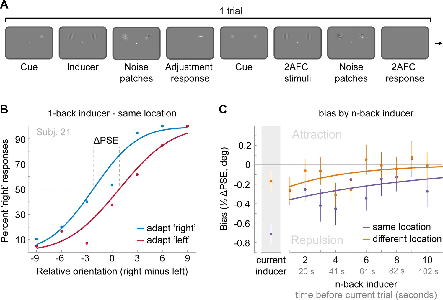
Task and results of Experiment 4: The long-term stimulus history directly biases the perceived orientation of current stimuli.
(A) Observers were cued to reproduce one of two Gabor stimuli by adjusting a response bar (adjustment response). Subsequently, two new Gabor stimuli appeared at priorly cued locations in the left and right visual field. Those stimuli could appear either at the same locations as the previous stimuli or 10 visual degrees above or below. Observers had to judge which of the two new stimuli was oriented more clockwise (2AFC). Similar to the previous experiments, all Gabor stimuli were followed by noise masks. (B) Psychometric curves for the 2AFC judgments of one example observer. We expressed the probability of a ‘right’ response (y-axis) as a function of the orientation difference between right and left 2AFC stimuli (x-axis). For positive x-values, the right stimulus was oriented more clockwise. We binned the trials in two bins according to the expected influence of repulsive adaptation to the inducer stimulus. Blue data points represent trials in which repulsive adaptation, away from the inducer, would favor a ‘right’ response, while red data points represent trials in which it would favor a ‘left’ response. The example observer exhibits a repulsive adaptation bias. We quantified the magnitude of the bias as the difference in the points of subjective equality between ‘adapt right’ and ‘adapt left’ curves (ΔPSE) divided in half. This value indicates how much a 2AFC stimulus is biased by a single inducer stimulus. (C) Bias exerted by the current inducer (gray shaded box, same data as in Experiment 2 by Fritsche et al., 2017) and inducers of the 10 preceding trials. Previous inducer stimuli exert a repulsive bias on the current 2AFC stimuli, specifically when past inducer and current 2AFC stimuli were presented at an overlapping spatial location. This bias appears to decay exponentially for inducers encountered further in the past. Note that while current inducers were always oriented ±20° from the subsequent 2AFC stimulus, constituting an optimal orientation difference for eliciting adaptation biases (e.g. see Figure 2B), relative orientations of previous inducers ranged from −49 to 49°, and thus presented overall less effective adaptor stimuli. This may explain the discontinuity in the magnitude of repulsion exerted by the current and previous trial inducer. Data points show group averages and error bars present SEMs.
-
Figure 5—source data 1
Task and results of Experiment 4: The long-term stimulus history directly biases the perceived orientation of current stimuli.
The source data file contains two csv files with estimated biases exerted by the previous 10 inducer stimuli, when the inducer was presented at the same or different spatial location, respectively (participants x n-back inducer).
- https://cdn.elifesciences.org/articles/55389/elife-55389-fig5-data1-v2.zip
Figure 6
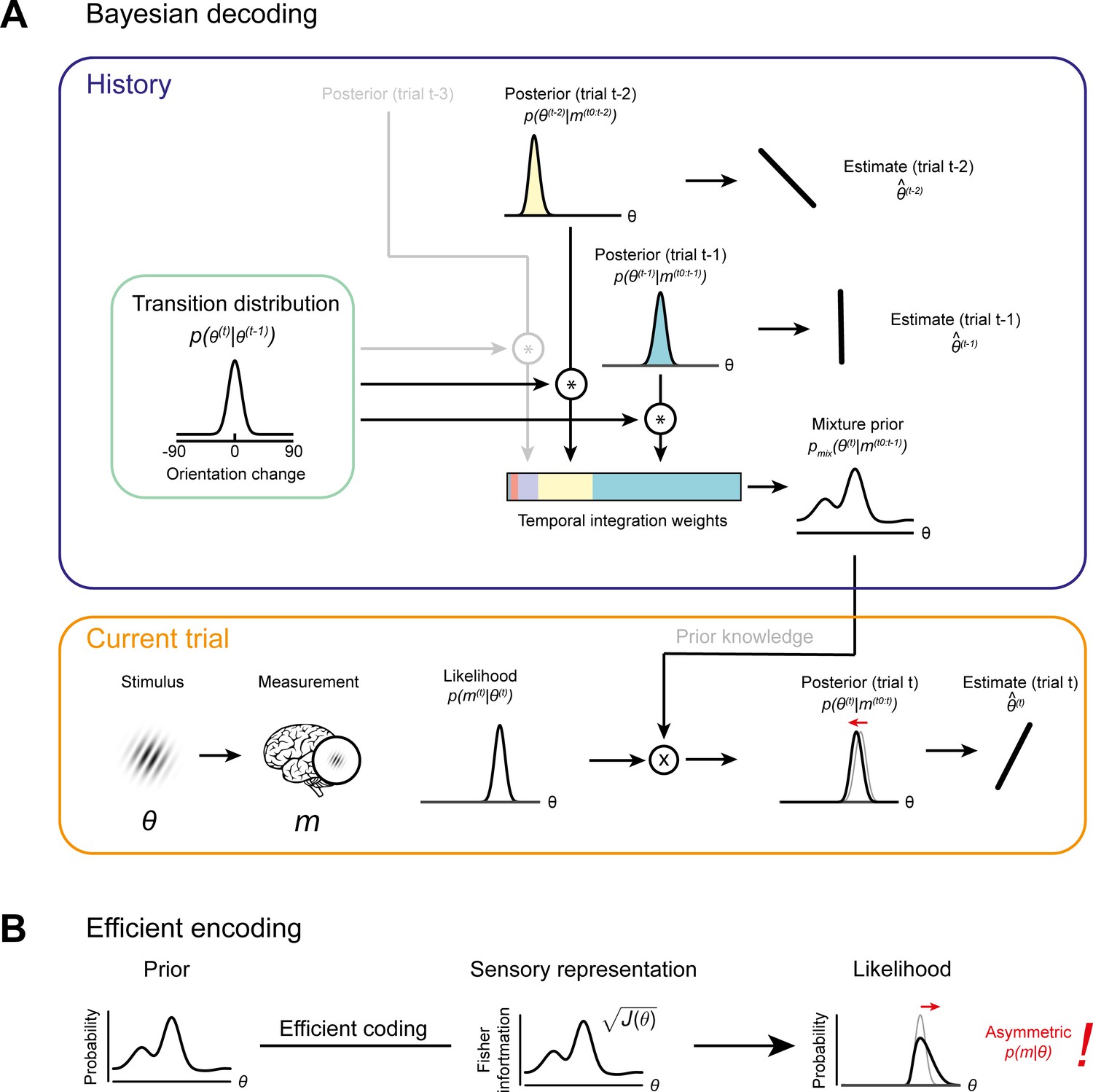
Bayesian decoding and efficient encoding of orientation information in a stable environment.
(A) Bayesian decoding. Orange box: The observer encodes a grating stimulus with orientation θ into a noisy measurement m. Since the noisy measurement is uncertain, it is consistent with a range of orientations, described by the likelihood function. The likelihood is combined with prior knowledge to form a posterior, which describes the observer’s knowledge about the current stimulus orientation. The final orientation estimate is taken as the posterior mean. Blue box: In a stable environment, the observer can leverage knowledge about previous stimuli for improving the current estimate. To predict the current stimulus orientation, the observer combines a model of orientation changes in a stable environment, represented by a transition distribution (green box), with knowledge about previous stimuli, that is previous posteriors. Predictions based on previous stimuli are integrated into recency-weighted mixture prior, using exponential integration weights. This mixture prior is subsequently used for Bayesian inference about the current stimulus. (B) Efficient encoding. The observer maximizes the mutual information between the sensory representation and physical stimulus orientations by matching the encoding accuracy (measured as the square root of Fisher information J(θ)) to the prior probability distribution over current stimulus orientations. In a stable environment, this prior distribution can be informed by previous sensory measurements. With some assumptions about the sensory noise characteristics (see Materials and methods), the likelihood function of new sensory measurements is fully constrained by the Fisher information. The likelihood function is typically asymmetric, with a long tail away from the most likely predicted stimulus orientation. For details see Materials and methods and Wei and Stocker, 2015.
Figure 7 with 5 supplements
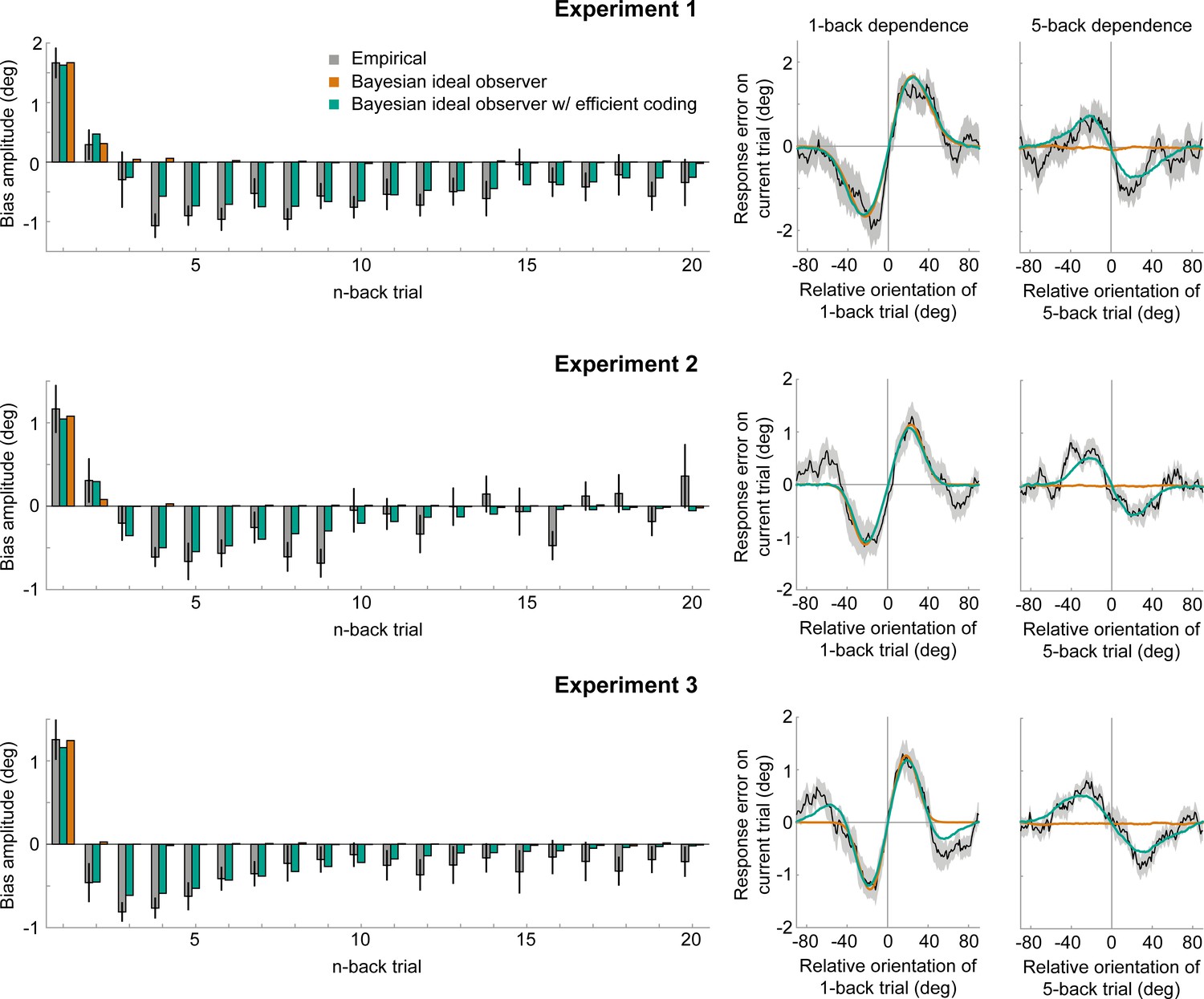
Empirical biases and ideal observer predictions.
Left column: An observer with efficient encoding and history-dependent Bayesian decoding (green) accurately captures the empirical magnitudes of short-term attractive and long-term repulsive biases exerted by the 1- to 20-back trials of Experiment 1–3 (grey). In contrast, an observer with Bayesian decoding (orange) only produces positive biases, but cannot capture the long-term repulsive biases. For each experiment, model bias amplitudes were estimated by simulating the observer model with the best fitting set of parameters on the stimulus sequences shown to human participants, and fitting the resulting model response errors with a Derivative-of-Gaussian (DoG) curve. Analogous to the analysis of human behavior, the amplitude parameter of the DoG curve was taken as the bias amplitude. Error bars represent 1 SD of the bootstrap distribution of the empirical data. Right column: Both attractive (left) and repulsive biases (right) of the ideal observer model with efficient encoding and Bayesian decoding (green) closely follow the average biases of human participants (black). The observer with Bayesian decoding (orange) does not produce repulsive biases. Black shaded regions show the SEMs of the empirical data. Model fits to the full range of 1- to 20-back conditioned response errors are shown in Figure 7—figure supplements 1 and 2. A comparison of cross-validated prediction accuracies of the different models is shown in Figure 7—figure supplement 3. The best fitting parameters of the observer model with efficient encoding and history-dependent Bayesian decoding are reported in Figure 7—figure supplement 5.
-
Figure 7—source data 1
Empirical biases and ideal observer predictions.
The source data file contains csv files with the empirical bias amplitudes of 1- to 20-back stimuli, as well as the predicted bias amplitudes of the ideal observer with efficient encoding and Bayesian decoding and the observer with Bayesian decoding alone. Three separate files are provided for Experiment 1–3, respectively. Furthermore, for each experiment we provide two mat files with the model fitting results of the two ideal observer models.
- https://cdn.elifesciences.org/articles/55389/elife-55389-fig7-data1-v2.zip
Figure 7—figure supplement 1

Serial dependence biases of an ideal observer with efficient encoding and history-dependent Bayesian decoding (green).
The model can accurately capture the tuning profile of short-term attraction and long-term repulsion biases across Experiments 1–3. Model biases were computed by simulating the ideal observer model on the stimulus sequences shown to human participants. Human serial dependence biases are shown in black. Shaded regions denote SEMs of the empirical data.
Figure 7—figure supplement 2
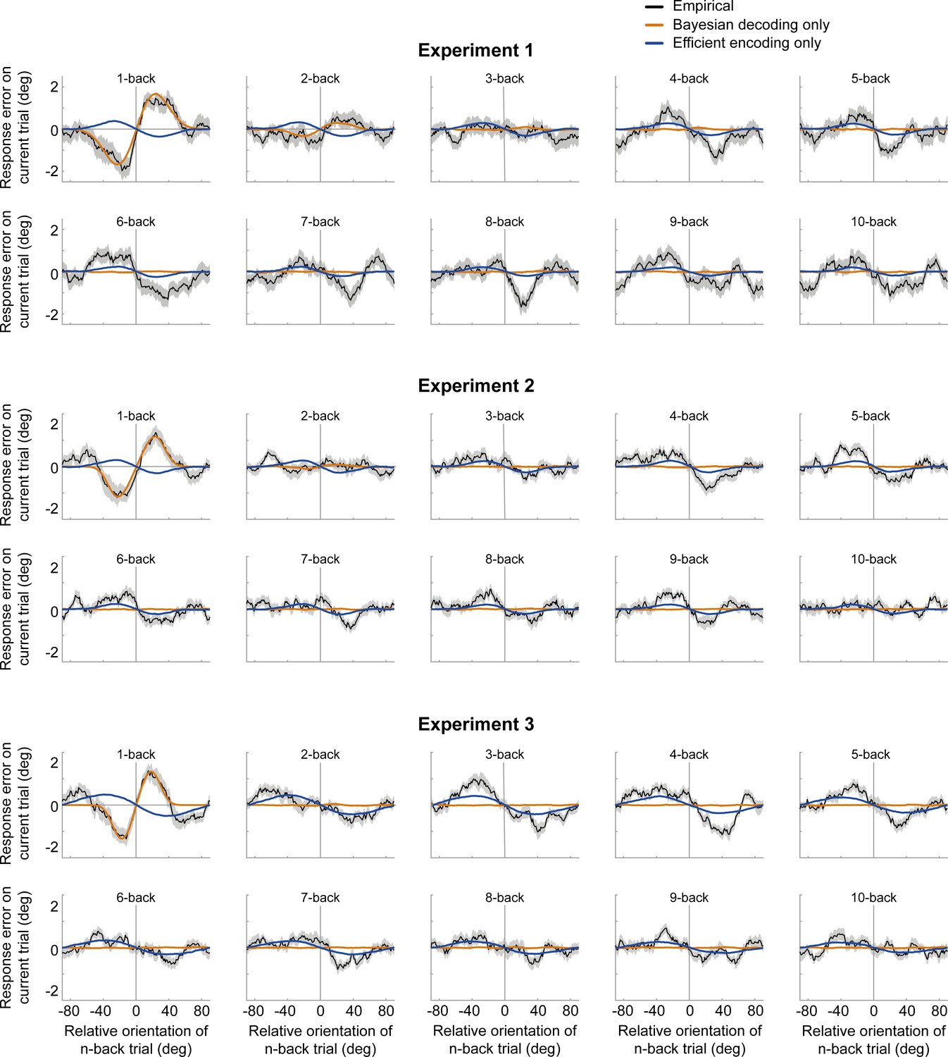
Serial dependence biases of an ideal observer, in which sensory history influenced only Bayesian decoding (orange) or only efficient encoding (blue).
Neither of the models can account for both attractive and repulsive biases. While the observer with Bayesian decoding can only produce attraction biases, the observer with efficient encoding only exhibits repulsion. Model biases are computed by simulating the ideal observer model on the stimulus sequences shown to human participants. Human serial dependence biases are shown in black. Shaded regions denote SEMs of the empirical data.
Figure 7—figure supplement 3
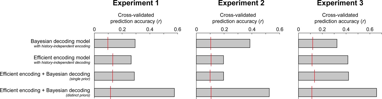
Cross-validated prediction accuracies of the four different observer models.
Across all three experiments, an ideal observer model with efficient encoding and Bayesian decoding optimized according to distinct priors (distinct transition distributions and integration time constants) provided the best fits to the held-out testing data. It consistently outperformed an ideal observer model in which encoding and decoding were based on the same predictions (single prior), or models in which the sensory history influenced only Bayesian decoding or only efficient encoding. Importantly, those models could not qualitatively account for all aspects of the empirical bias pattern, being limited to producing only attractive or only repulsive biases. A baseline level of chance prediction accuracy of each model is indicated by the red lines. To this end, we randomly permuted the models’ predicted responses to the stimuli in the testing dataset, thereby abolishing the trial correspondence between model and participant errors, and computed the correlation between the resulting permuted model predictions and observed serial dependence curves. This procedure was repeated 1000 times. The red line indicates the 95th percentile of the resulting permutation distribution.
Figure 7—figure supplement 4

Normalized variability of estimation response errors as a function of the orientation difference between current and n-back trial.
Variability of estimation response errors was quantified by computing each participant’s standard deviation of estimation response errors in a 30° sliding window over relative orientation differences between current and n-back trial. The resulting conditional response variability estimates were normalized by subtracting each participant’s mean response variability before averaging across participants. Across all three estimation experiments, there was a clear reduction in response variability when current and previous stimuli had similar orientations (left column, thin black line) and this pattern was well captured by a second-derivative-of-a-gaussian curve (bold black line). The amplitude parameter a of the gaussian derivative model quantifies the reduction of response variability at 0° relative orientation difference. While for some n-back trials there appears to be a small reduction in response variability (e.g. 4-back trials, middle column), temporally more distant trials show no consistent effect overall (right column). Shaded error regions around the group-averaged example curves depict SEMs. Error bars on amplitude estimates depict 1 SD of the bootstrapped amplitude distribution, resampling participants with replacement.
Figure 7—figure supplement 5
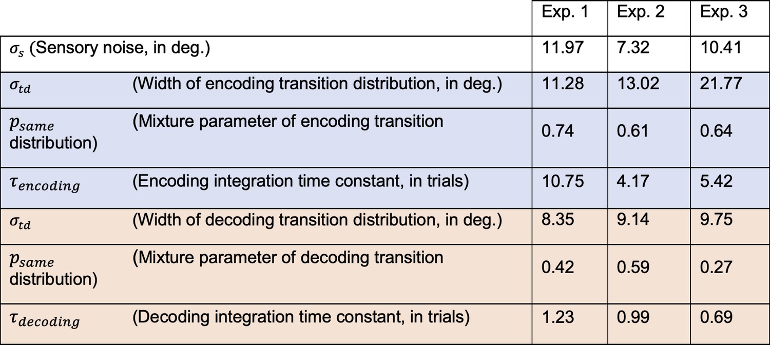
Best fitting parameters of the observer model with efficient encoding and history-dependent Bayesian decoding (Full efficient-encoding-Bayesian-decoding model).
Parameters of the encoding and decoding stages are presented in the blue and red shaded cells, respectively. Note that exponential integration time constants are fitted in units of trials, and can be converted into an estimate of seconds by multiplying with the average trial duration of the respective experiment (average trial durations: Exp. 1: 5.38 s; Exp. 2: 6.55 s; Exp. 3: 8.25 s).
Additional files
Download links
A two-part list of links to download the article, or parts of the article, in various formats.
Downloads (link to download the article as PDF)
Open citations (links to open the citations from this article in various online reference manager services)
Cite this article (links to download the citations from this article in formats compatible with various reference manager tools)
A Bayesian and efficient observer model explains concurrent attractive and repulsive history biases in visual perception
eLife 9:e55389.
https://doi.org/10.7554/eLife.55389


