The effects of chloride dynamics on substantia nigra pars reticulata responses to pallidal and striatal inputs
- Department of Mathematics, University of Pittsburgh, United States
- Center for the Neural Basis of Cognition, United States
- Department of Biological Sciences, Carnegie Mellon University, United States
Figures
Figure 1
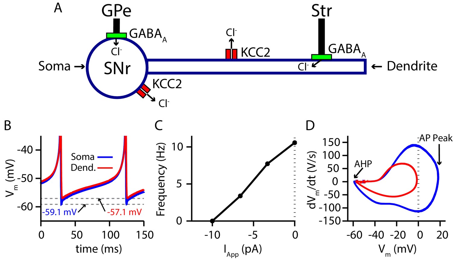
Two-compartment SNr model neuron includes currents that affect and produces appropriate dynamics.
(A) Schematic diagram of the model. (B) Tonic spiking voltage traces for both compartments, with minimum voltages labeled. (C) Model f-I curve. (D) Phase plot of the rate of change of the membrane potential () against the membrane potential (Vm) showing afterhyperpolarization (AHP) and spike height (AP Peak) for both compartments.
Figure 2
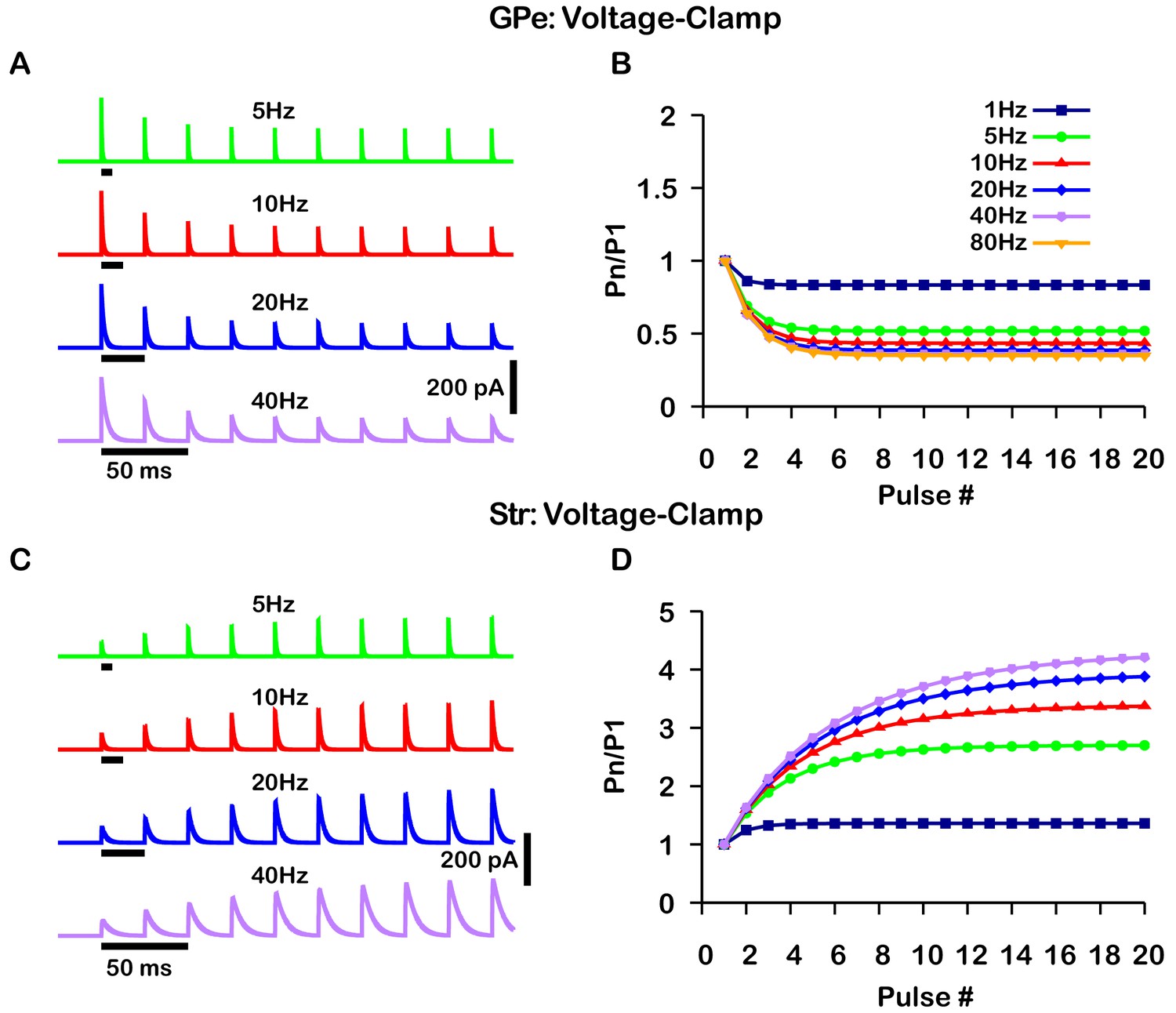
Simulated short-term synaptic depression and facilitation of GABAergic synapses originating from GPe neurons of the indirect pathway (A and B) and Str neurons of the direct pathway (C and D) under voltage clamp.
For the GPe and Str simulations, the left traces (A and C) show current and right panels (B and D) show the pared pulse ratios (PPR) resulting from repeated synaptic stimulation at different frequencies. The amplitude of each IPSC (Pn) was normalized to the amplitude of the first evoked IPSC (P1). For this set of simulations the membrane potential was held at and for the somatic and dendritic compartments was held fixed at –72 mV. Model parameters and behavior were tuned to match voltage-clamp data from Connelly et al., 2010.
Figure 3
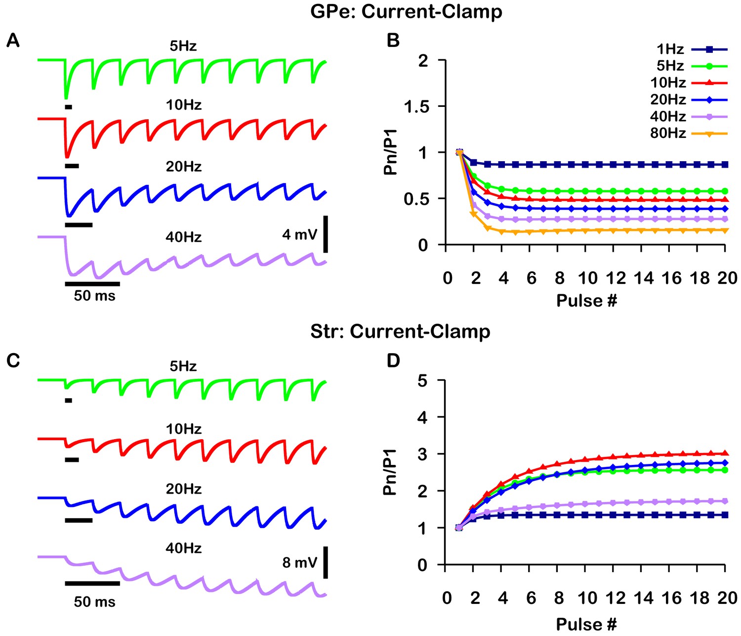
Simulated short-term synaptic depression and facilitation of GABAergic synapses originating from GPe neurons of the indirect pathway (A and B) and Str neurons of the direct pathway (C and D) under current clamp.
For the GPe and Str simulations, the left traces (A and C) show voltage and right panels (B and D) show the pared pulse ratios (PPR) resulting from repeated synaptic stimulation at different frequencies. The amplitude of each IPSP (Pn) was normalized to the amplitude of the first evoked IPSP (P1). For this set of simulations was tuned to set the resting membrane of the somatic compartment at . In both compartments was held fixed at –70 mV. Model performance is qualitatively, and somewhat quantitatively, similar to experimental current-clamp data (Lavian and Korngreen, 2016, Figures 2, 3).
Figure 4 with 1 supplement
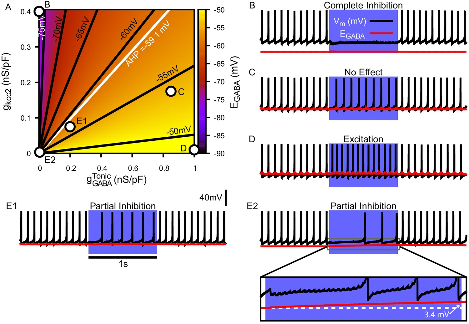
Tonic chloride conductance and extrusion capacity determine somatic and SNr responses to simulated 40 Hz GPe stimulation.
(A) Dependence of somatic on the tonic chloride conductance () and the potassium-chloride co-transporter KCC2 extrusion capacity (). (B–E) Examples of SNr responses to simulated indirect pathway stimulation at different positions in the 2D (,) parameter space, as labeled in panel (A). (E1 and E2) Notice the two distinct types of partial inhibition. Inset highlights the drift in during stimulation.
Figure 4—figure supplement 1
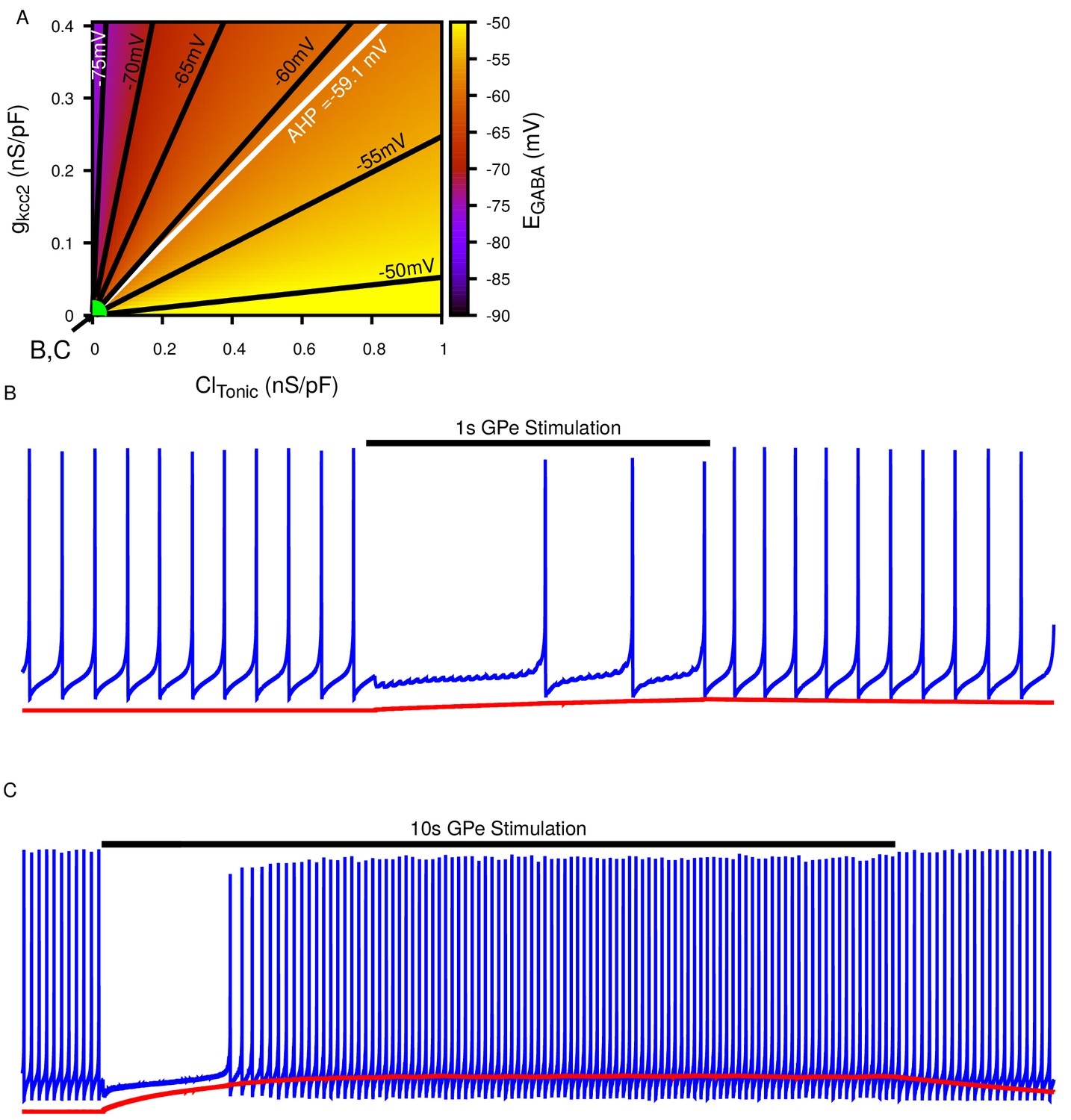
Biphasic SNr response to longer simulated GPe stimulation.
(A) Dependence of somatic on the tonic chloride conductance () and the potassium-chloride co-transporter KCC2 extrusion capacity () as previously shown in Figure 4A. (B) Example of ‘Partial Inhibition’ in response to 1 s of stimulation resulting due to a small accumulation of intracellular , as shown in Figure 4E2. (C) Example of longer 10 s stimulation resulting in larger accumulation resulting in a transition of from inhibitory to excitatory and thus causing a biphasic response in a simulated SNr neuron’s firing rate, as seen in 10 s stimulation experiments. and are the same in (B) and (C) and take the values indicated in (A). To generate the biphasic example the synaptic conductance was increased from 0.2 to 0.4 nS/pF.
Figure 5

Tonic chloride conductance and extrusion capacity determine dendritic and SNr responses to 20 Hz Str stimulation.
(A) Dependence of somatic on the tonic chloride conductance () and the potassium-chloride co-transporter KCC2 extrusion capacity (). (B–F) Examples of SNr responses to simulated indirect pathway stimulation at different locations in the 2D (,) parameter space. and for each example are indicated in panel (A). (E1 and E2) Notice the two distinct types of partial inhibition. Inset highlights the drift in during stimulation. (F) Example of a biphasic inhibition-to-excitation response elicited by increasing the stimulation frequency to 40 Hz under the same conditions shown in E2. Alternatively, same response could be elicited by increasing the synaptic weight (). .
Figure 6 with 2 supplements
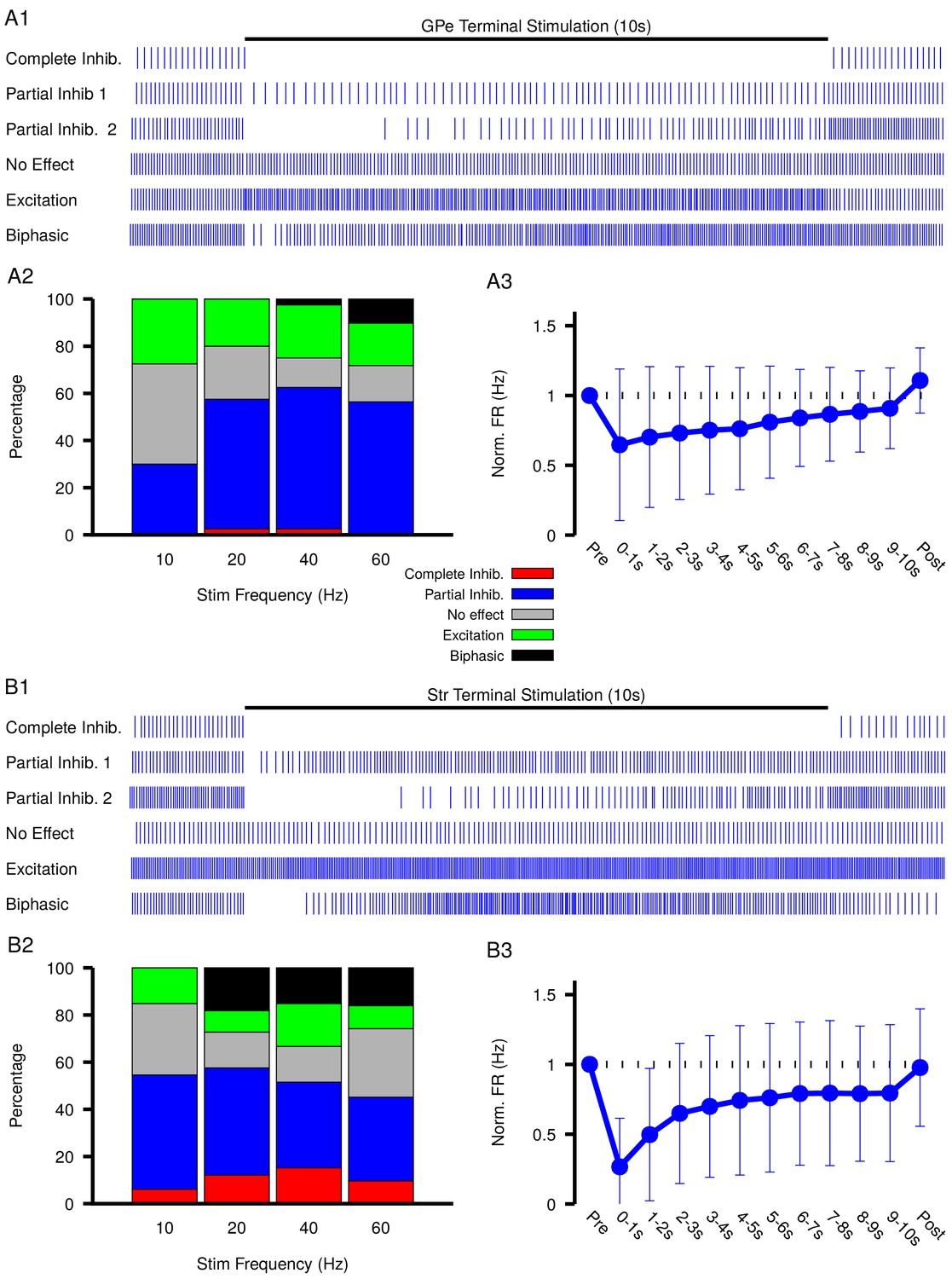
Characterization of experimentally observed SNr responses to optogenetic stimulation of (top) GPe and (bottom) Str projections to SNr in vitro.
(A1 and B1) Examples of response types observed for 10 s stimulation of GPe or Str projections. (A2 and B2) Quantification types of SNr response to optogenetic stimulation at varying frequencies (GPe: animals, 12 slices, 10 Hz, 20 Hz, and 40 Hz = 40 cells, 60 Hz = 39 cells; Str: animals, 12 slices, 10 Hz, 20 Hz, and 40 Hz = 33 cells, 60 Hz = 31 cells). (A3 and B3) Effect of GPe or Str stimulation on the firing rate of SNr neurons averaged across all trials for stimulation at 40 Hz. Error bars indicate the standard deviation. The 10 s stimulation period was broken into 1 s intervals to show the gradual weakening of inhibition during stimulation.
Figure 6—figure supplement 1
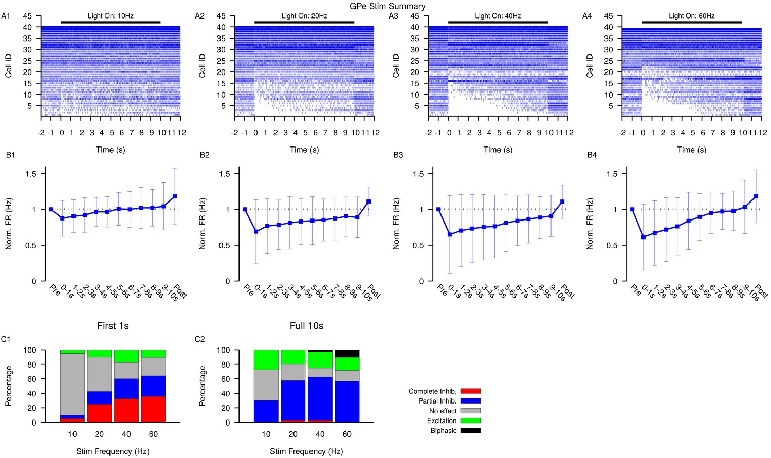
Summary of SNr responses to optogenetic stimulation of GPe synaptic terminals.
(A1–A4) Raster plots of spiking sorted by the duration of the pause in spiking at the start of the stimulation period for all SNr neurons tested. (B1–B4) Effect of GPe stimulation on the firing rate of SNr neurons averaged across all neurons and each stimulation frequencies tested. Error bars indicate SD. (C1 and C2) Quantification of types of SNr responses to optogenetic stimulation for varying frequency characterized in the first (C1) 1 s or the full (C2) 10 s. Notice that fewer neurons are completely inhibited in the full period and some biphasic responses emerge.Str: animals, 12 slices, 10 Hz, 20 Hz, and 40 Hz = 33 cells, 60 Hz = 31 cells.
Figure 6—figure supplement 2
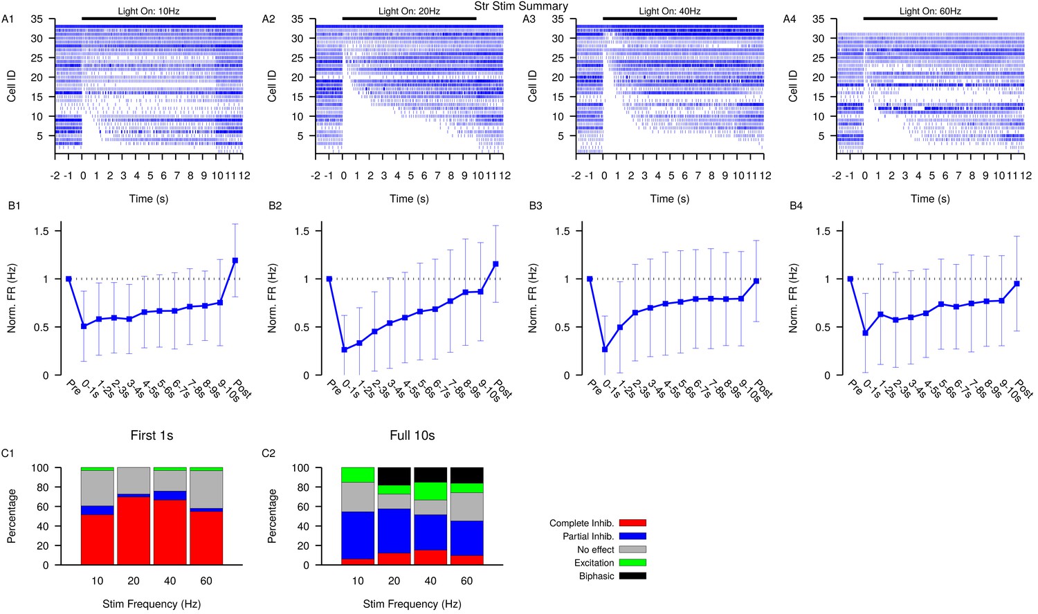
Summary of SNr responses to optogenetic stimulation of Str synaptic terminals.
(A1–A4) Raster plots of spiking sorted by the duration of the pause in spiking at the start of the stimulation period for all SNr neurons tested. (B1–B4) Effect of Str stimulation on the firing rate of SNr neurons averaged across all neurons and each stimulation frequencies tested. Error bars indicate SD. (C1 and C2) Quantification of types of SNr responses to optogenetic stimulation for varying frequency characterized in the first (C1) 1 s or the full (C2) 10 s. Notice the decrease in the number of completely inhibited neurons and increase in the number of biphasic responses in the full 10 s period. Str: animals, 12 slices, 10 Hz, 20 Hz, and 40 Hz = 33 cells, 60 Hz = 31 cells.
Figure 7
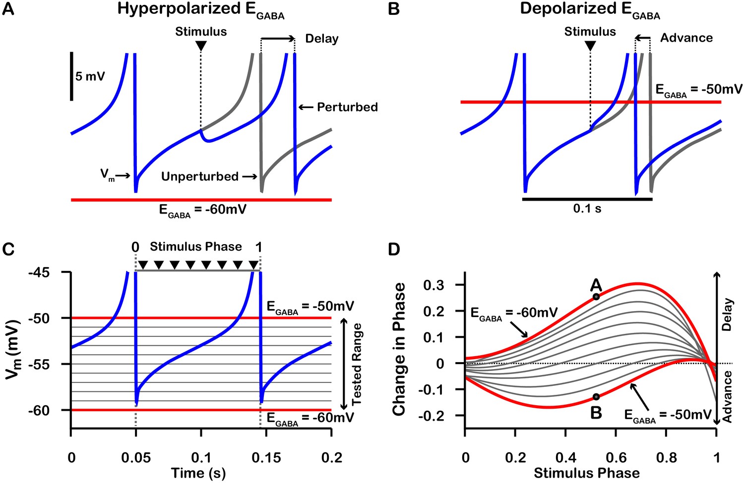
Phase response curves (PRCs) of the model SNr neuron depend on .
(A and B) Example traces illustrating the effect of a single GABAergic synaptic input on the phase of spiking in a simulated SNr neuron for hyperpolarized and depolarized , respectively. (C) For an ongoing voltage oscillation of a spiking SNr neuron (blue trace), we define a phase variable as progressing from 0 immediately after a spike to one at the peak of a spike. As is varied from –60 mV to –50 mV, progressively more of the SNr voltage trace lies below , where GABAergic inputs have depolarizing effects. (D) PRCs computed for a model SNr neuron in response to GABAergic input stimuli arriving at different phases of an ongoing SNr oscillation. As is varied from –60 mV to –50 mV, the PRC transitions from a curve showing a delay of the next spike for most stimulus arrival phases, through some biphasic regimes, to a curve showing an advance of the next spike for almost all possible phases. In panel D, the A and B labels at approximately 0.5 phase on the and PRCs correspond to the examples shown in panels A and B. The conductance of the synaptic input was fixed at 0.1 nS/pF in order to produce deflections in Vm for hyperpolarized that are consistent with data presented in Higgs and Wilson, 2016.
Figure 8 with 1 supplement
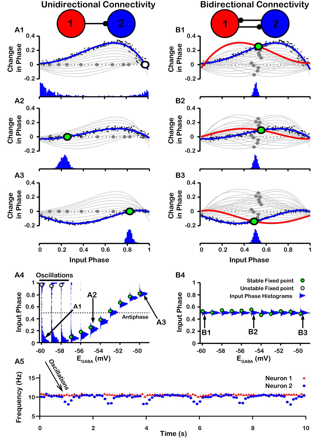
Effect of on SNr synchrony in a unidirectional (left) and bidirectional (right) synaptically connected two-neuron network.
(A1-A3 and B1-B3) (Top) Identification of PRC fixed points and (Bottom) histogram of the timing of synaptic inputs in the phase of neuron 2 (Input Phase) as a function of . Recall that positive changes in phase correspond to delays. (A1,B1) ; (A2,B2) ; (A3,B3) . Black dots indicate dataset used to generate PRC in red/blue. Stable and unstable fixed points are indicated by green and white filled circles, respectively. For reference, all PRCs and fixed points are included in gray for all values of tested. (A4,B4) Effect of on SNr phase locking. Blue histograms show the distribution of synaptic inputs relative to the phase of neuron 2 (input phase) for the two network simulations for different levels of . Green and white filled circles indicate the stable and unstable locking predicted by analysis of PRCs. Note the unstable fixed points for the lowest values of in the unidirectional case. (A5) In the unidirectional case, slow 1 Hz oscillations in the frequency of neuron 2 arise due to phase slipping at hyperpolarized values of .
Figure 8—figure supplement 1
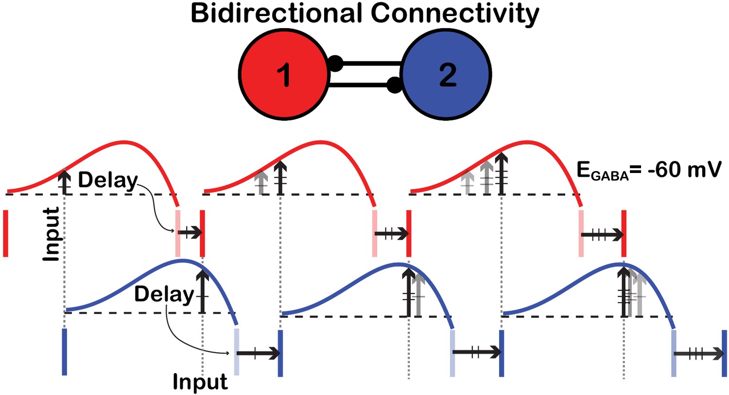
Schematic illustration of the convergence toward anti-phase locking in a birectionally coupled pair of SNr neurons.
Each vertical, deeply colored bar denotes a spike time of the cell with that color (red or blue). Following the spike time of each cell, the PRC for that cell is shown (the PRCs for are used). The spike time of one cell becomes the input time to the other, target cell (‘Input’). The height of the PRC for the target cell at the arrival time of its input determines the delay (‘Delay’) until its next spike. Each pale vertical bar shows the time when that next spike would have occurred had the corresponding cell not received an input; each horizontal arrow shows how the delay due to input perturbs the cell’s actual next spike time and determines the timing of the next input to the other cell. Over successive spikes and delays, the relative phases of the cells drift, such that the cells’ spike times approach the fully anti-phase locked state, in which each cell spikes, and sends input to the other cell, half-way through each interspike interval.
Figure 9

Characterization of phase slipping oscillations in the unidirectionally connected two-neuron network.
(A) Illustration of the phase of the postsynaptic neuron at the moment when it receives each input from the presynaptic neuron (input phase) for the unidirectionally connected two neuron network as a function of time for . Dots denote phases of the postsynaptic neuron when the presynaptic neuron spikes. The phase value of 1 corresponds to the postsynaptic neuron being at spike threshold. Insets show the timing of the presynaptic neuron spike (black triangle/dashed line), the phase of the postsynaptic neuron spike after it receives the input (blue), and the spike train of the postsynaptic neuron in the absence of input (gray). The red cycle is used in B. (B) Overlay of the PRC generated for and the resulting progression of phase for one full phase slipping oscillation. Light gray dots indicate the data points used to generate the blue PRC. Recall that positive changes in phase correspond to delays. (C) The frequency of phase slipping increases as decreases, with a steeper relationship for larger synaptic weight () between the SNr neurons. .
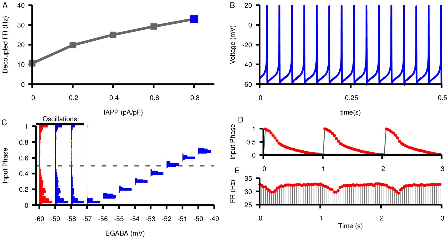
Figure 10 with 7 supplements

Effects of changing the presynaptic firing rate on synchrony and postsynaptic oscillations in a feed-forward SNr neuron pair.
(A) Tuning curve for presynaptic firing rate (FR) versus applied current, . Dashed line indicates the baseline firing rate (10.5 Hz) with no applied current. (B) Histograms of the input phase in the postsynaptic neuron under baseline conditions (). (C1–C4) Input phase histograms for different presynaptic firing rates (9.76 Hz, 10.15 Hz, 10.91 Hz, 11.26 Hz from left to right). ranges are not the same in all panels. Regions of phase slipping (PS) and phase advancing (PA) oscillations are each indicated by a solid horizontal bar. Example oscillations in input phase (D1–D4) and postsynaptic firing rate (E1–E4) at specific values of for different presynaptic firing rates highlighted in red for the corresponding D panels. Notice that the PA oscillations in C1-2 and D1-2 result in periodic increases in the postsynaptic firing rate in E1-2 whereas PS oscillations in C3-4 and D3-4 result in periodic decreases in firing rate in E3-4.
Figure 10—figure supplement 1
The relationship between and phase locking and the emergence of slow oscillations are maintained at least up to in vivo SNr firing rates.
(A) Relationship between applied current () and the firing rate of an isolated SNr model neuron. (B) Example voltage trace for a simulated neuron firing at 33.0 Hz with . (C) Histograms of input phase in the two SNr neurons with unidirectional (feed forward) connectivity as a function of . Oscillations occur for and strict phase locking for . (D) Example plot showing slow oscillations in the phase of the presynaptic neuron at which the postsynaptic spike occurs (input phase) over time. (E) Example slow oscillations in the instantaneous firing rate of the postsynaptic neuron. in panels D and E.
Figure 10—figure supplement 2
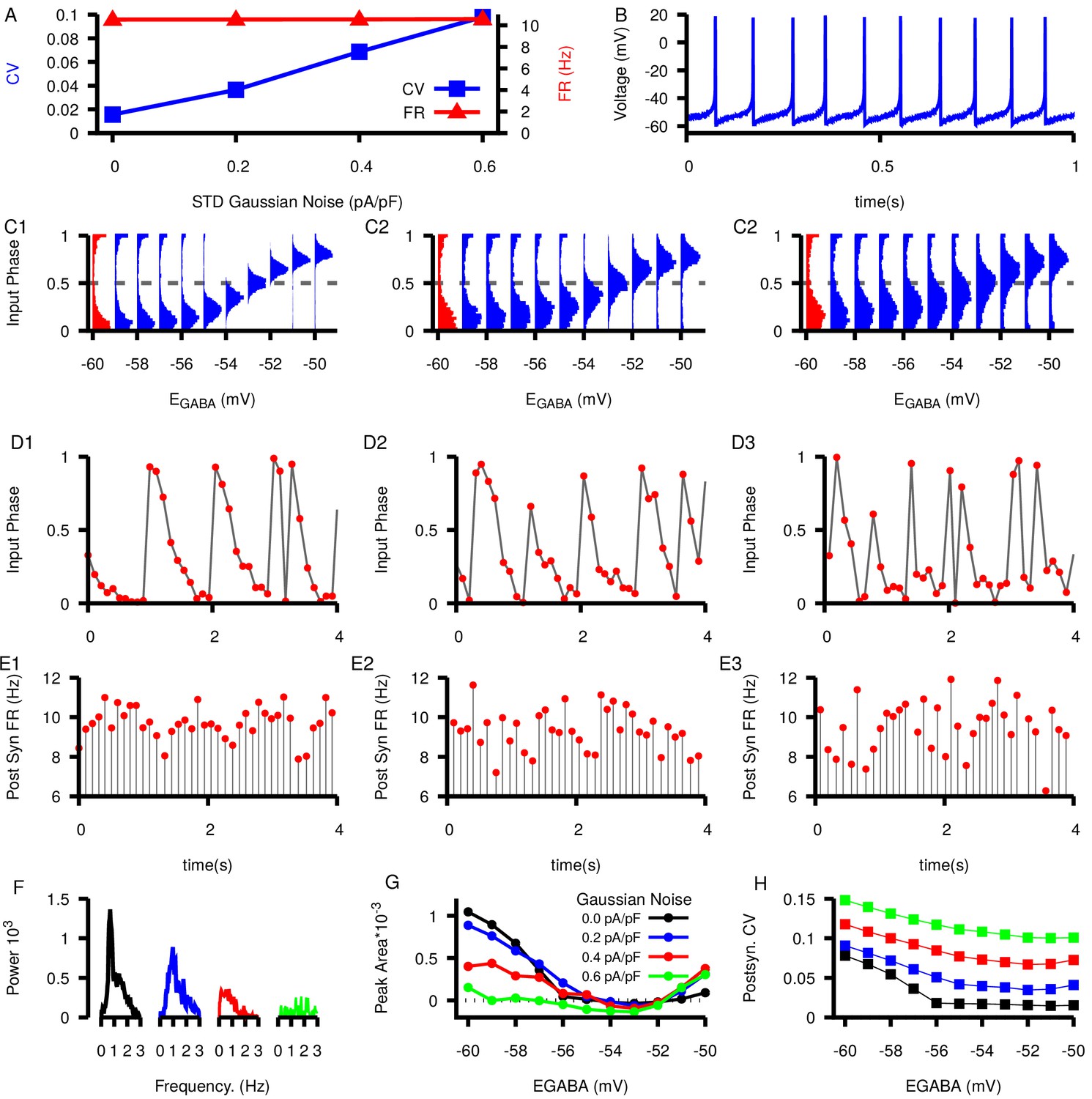
Effect of increasing noise on SNr phase relationships as a function of .
(A) Dependence of CV (blue) and firing rate (red) of model SNr neuron on applied noise amplitude. (B) Example voltage trace at the highest level of added Gaussian noise () and . (C) Relationships between and input phase distributions for increasing Gaussian noise: (C1) , (C2) , and (c3) . (D–E) Example slow oscillations in the input phase (D1–D3) and the post synaptic firing rate (E1–E3). values in the example traces are indicated by red histograms in the corresponding panel in (C). (F1) Example power spectrum curves in the 0–3 Hz range with 0.0, 0.2, 0.4, and 0.6 pA/pf of Gaussian noise and . In each case, results shown are remaining power after subtraction of the mean power in the 3–4 Hz range. (G) Area of the power spectrum peak as a function of and applied Gaussian noise. (H) CV in the postsynaptic neuron as a function of and added Gaussian noise. Note that postsynaptic CVs exceed those reported in the literature when we take a noise amplitude of 0.6 pA/pf, suggesting that this value may be excessive.
Figure 10—figure supplement 3
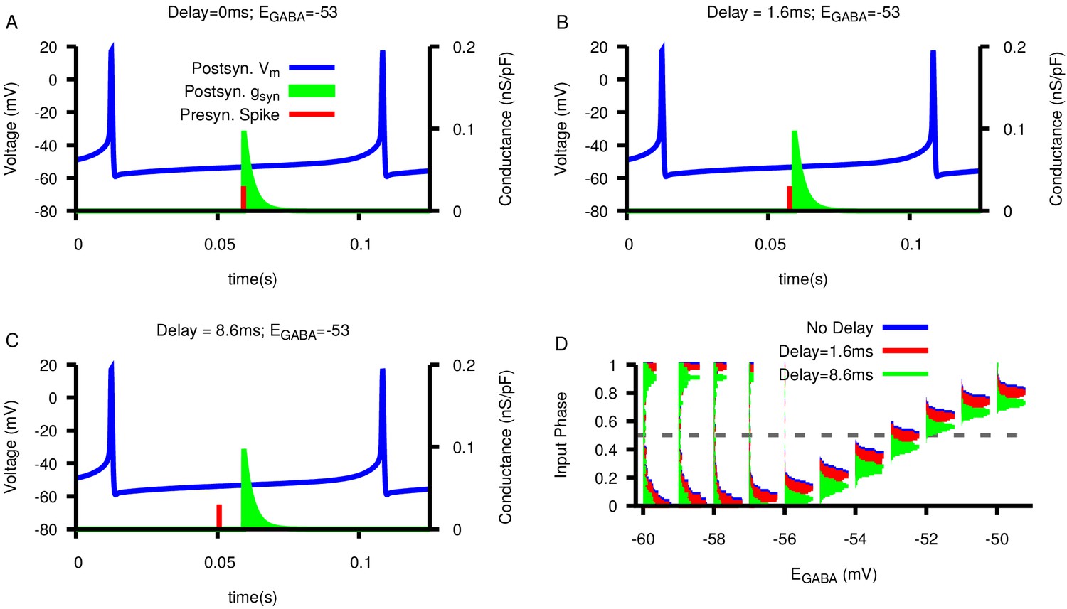
Effect of synaptic delay on the relationship between and presynaptic/postsynaptic phase locking.
(A–C) Examples of synaptic delays of increasing magnitude: 0 mS, 1.6 mS, and 8.6 mS, respectively. (D) Histogram of input phase in the postsynaptic neuron as a function of and varying delay duration. Notice that delays do not strongly effect the neurons’ spiking relationship.
Figure 10—figure supplement 4
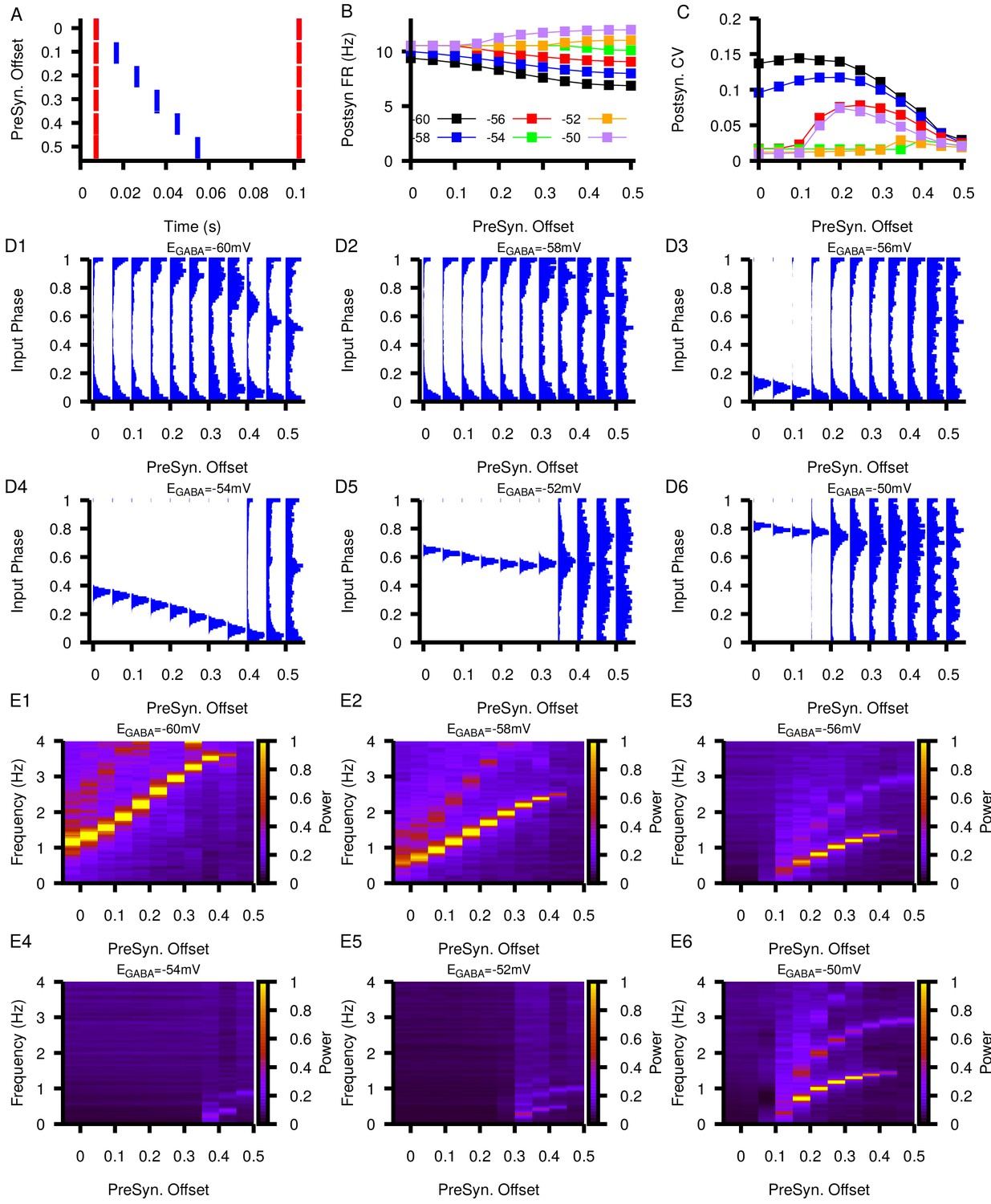
Relationship between postsynaptic firing properties as a function of and varying degrees of synchrony between two presynaptic neurons.
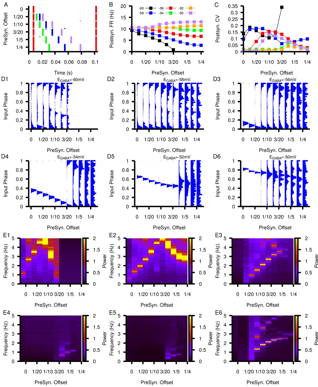
(A) Characterization of the varying degrees of presynaptic synchrony defined by the parameter presynaptic offset. The presynaptic offset is the phase difference between the first (red) and second (blue) presynaptic neuron. (B and C) Effect of varying presynaptic offset on postsynaptic (B) firing rate and (C) coefficient of variation (CV). (D1–D6) Input phase histograms for synaptic inputs in the postsynaptic neuron from the first presynaptic neuron as a function of the presynaptic offset and . (E1–E6) Power spectrum in the post synaptic neurons as a function of the presynaptic offset and .
Figure 10—figure supplement 5
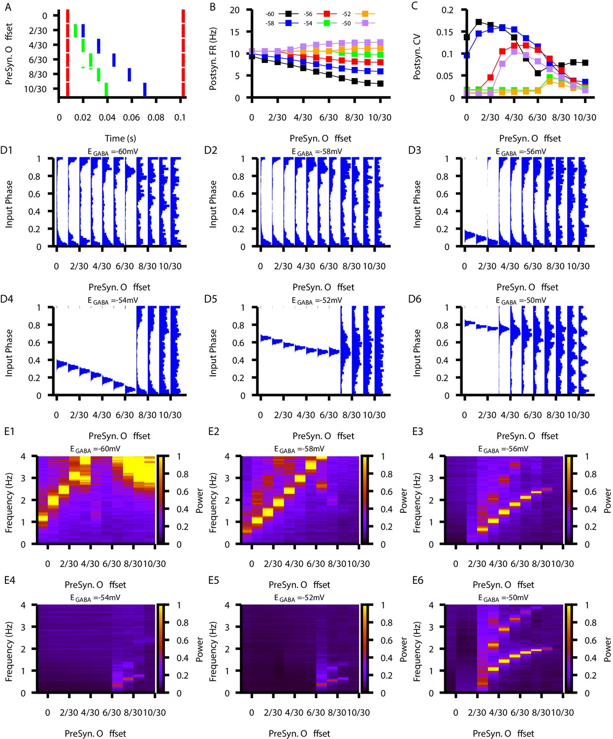
Relationship between postsynaptic firing properties as a function of and varying degrees of synchrony between three presynaptic neurons.
(A) Characterization of the varying degrees of presynaptic synchrony defined by the parameter presynaptic offset. The presynaptic offset is the phase difference between the first (red),second (green) and third (blue) presynaptic neuron. (B and C) Effect of varying presynaptic offset on postsynaptic (B) firing rate and (C) coefficient of variation (CV). (D1–D6) Input phase histograms for synaptic inputs in the postsynaptic neuron from the first presynaptic neuron as a function of the presynaptic offset and . (E1–E6) Power spectrum in the post synaptic neurons as a function of the presynaptic offset and .
Figure 10—figure supplement 6
Relationship between postsynaptic firing properties as a function of and varying degrees of synchrony between four presynaptic neurons.
(A) Characterization of the varying degrees of presynaptic synchrony defined by the parameter presynaptic offset. The presynaptic offset is the phase difference between the first (red),second (green),third (blue) and fourth (purple) presynaptic neuron. (B and C) Effect of varying presynaptic offset on postsynaptic (B) firing rate and (C) coefficient of variation (CV). (D1–D6) Input phase histograms for synaptic inputs in the postsynaptic neuron from the first presynaptic neuron as a function of the presynaptic offset and . (E1–E6) Power spectrum in the post synaptic neurons as a function of the presynaptic offset and .
Figure 10—figure supplement 7
Effects of varying on post synaptic dynamics in the three-neuron motif where neuron 1 projects to neuron 2 and neuron 3 and neuron 2 projects to neuron 3 (motif number 10 from Song et al., 2005).
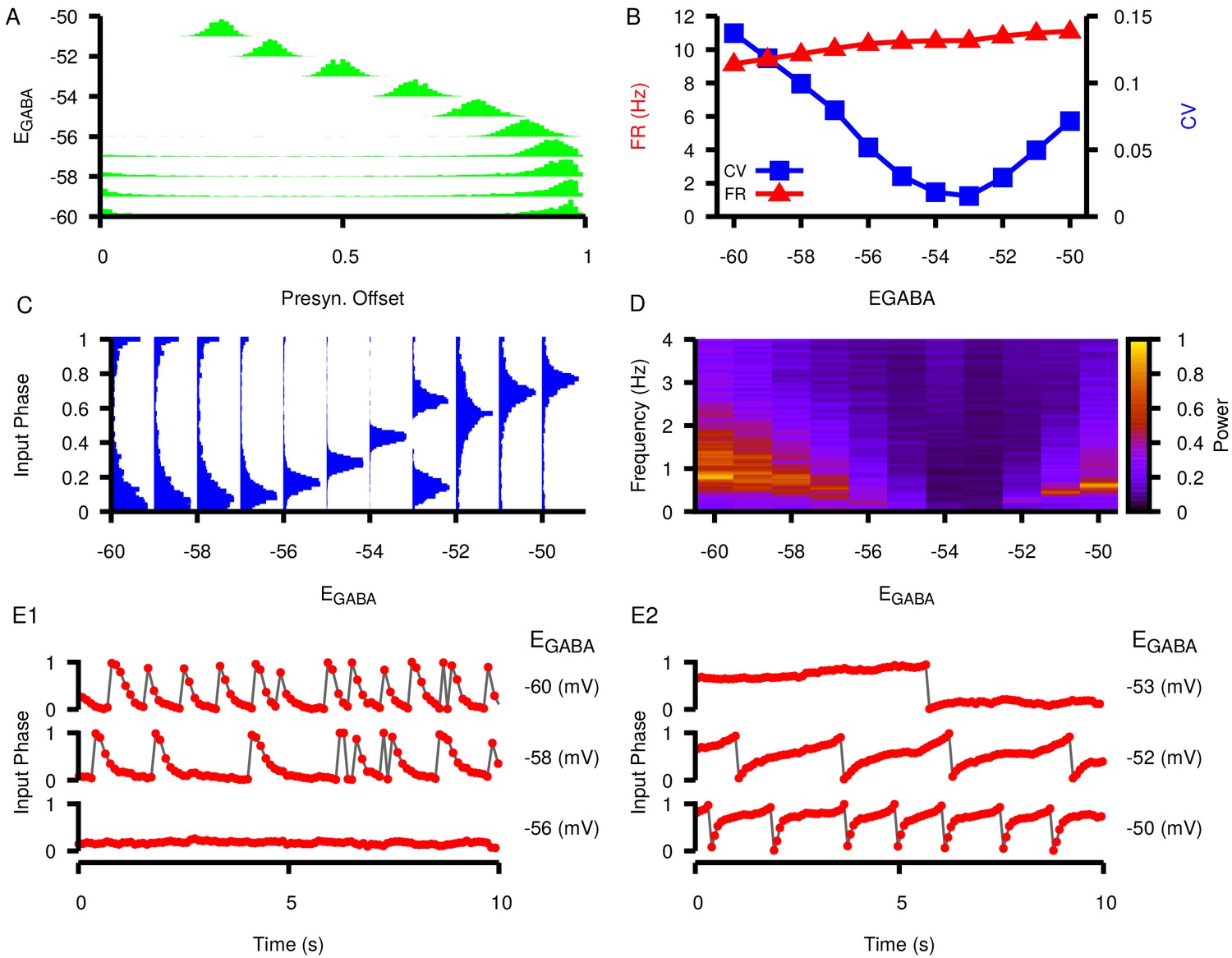
(A) Phase difference between the two presynaptic neurons (cell 1 and cell 2) as a function of . (B) Firing rate and coefficient of variation (CV) in the postsynaptic neuron (cell 3) as a function of . (C) Input phase histograms for synaptic inputs in the postsynaptic neuron from the first presynaptic neuron as a function of . (D) Power spectrum in the postsynaptic neuron as a function of . (E1 and E2) Example traces of the input phase relationship between the postsynaptic neuron and the first presynaptic neuron. The value of is indicated to the left of each trace.
Figure 11
Effect of varying in a network of 100 model SNr neurons with random, sparse connectivity.
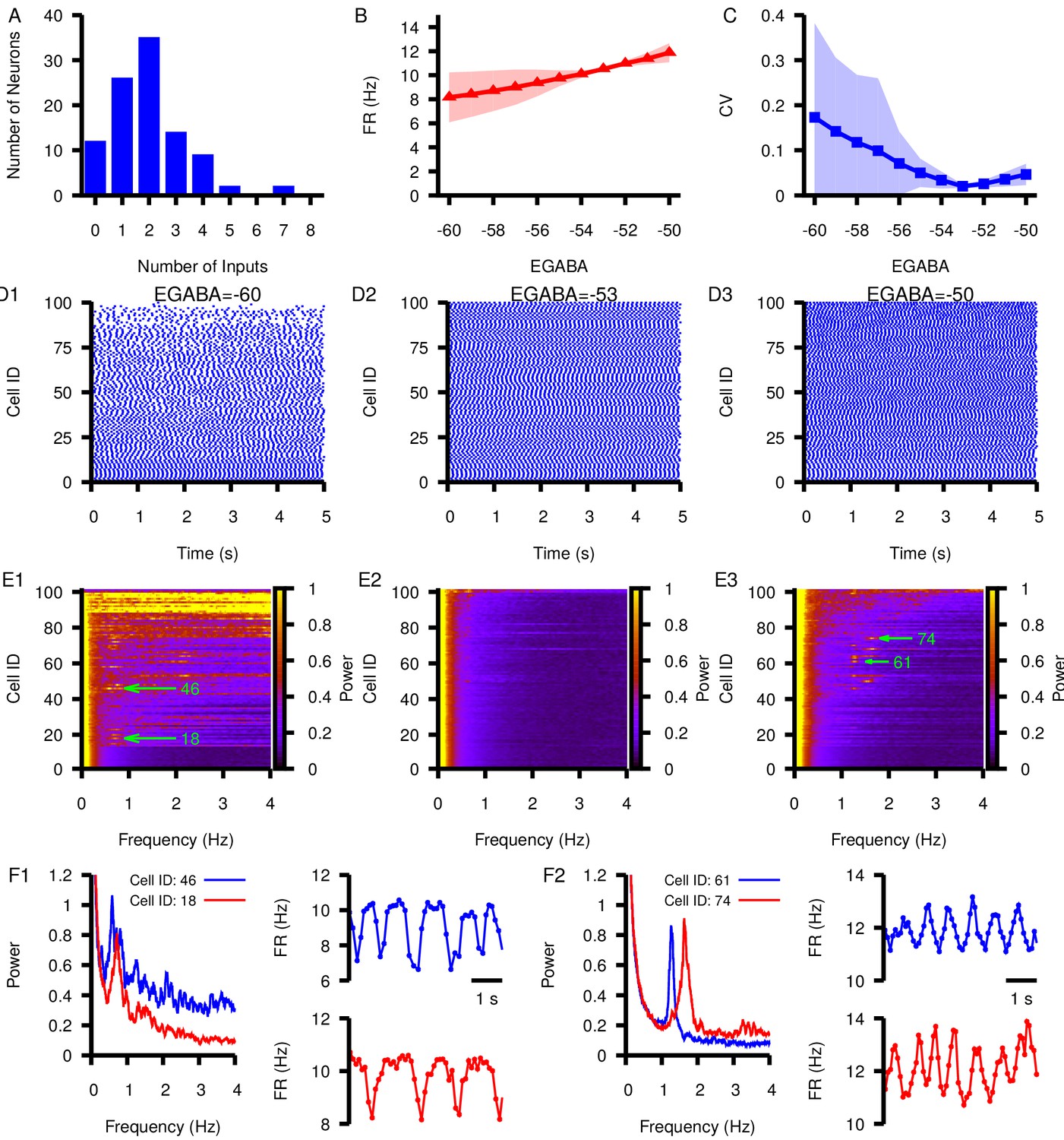
(A) Histogram showing the number of neurons receiving zero to eight synaptic inputs. (B) Mean network firing rate as a function of . (C) Mean network CV as a function of . Shaded regions in B and C represent standard deviation. (D1–D3) Example raster plots of spikes in the network for three different values of . (E1–E3) Power spectrum for each neuron in the network for the same three values of used in (D1–D3). Rows in D and E panels are sorted by the number of inputs from least (cell 1) to most (cell 100). Green arrows point out peaks in the power spectra of example neurons examined in the following panels. (F1 and F2) Left panel: Power spectrum for two example neurons with peaks indicating slow oscillations. Right panels: slow oscillation in the instantaneous firing rate in the two example neurons. These are shown for (F1) and for (F2).
Figure 12
Slow oscillations in the SNr seen under dopamine depleted conditions in vivo are suppressed by channelrhodopsin-2 optogenetic stimulation of GABAergic GPe terminals in the SNr.
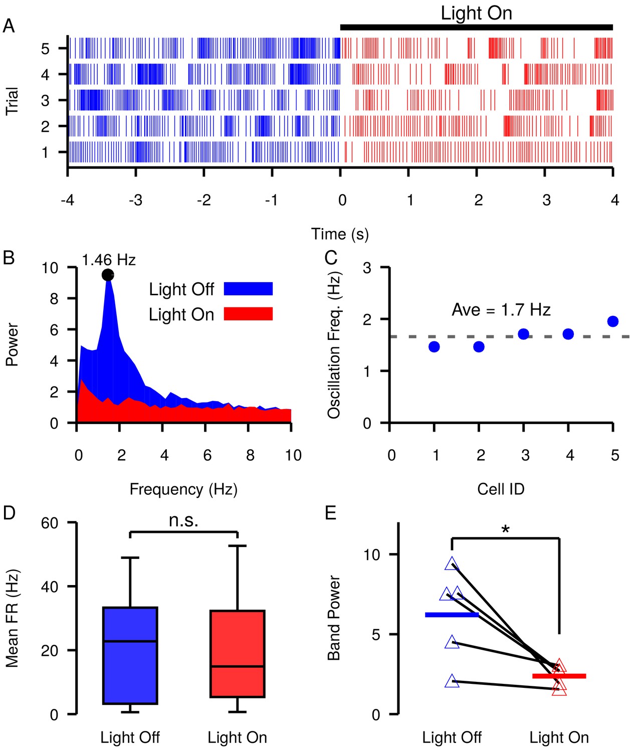
(A–B) Example (A) raster plot and (B) power spectrum of a single spiking unit in SNr without (blue) and with (red) optogenetic stimulation of GPe terminals over multiple trials. (C) Frequencies of slow oscillations in the 12 unit dataset before optogenetic stimulation. (D) Distribution of single unit firing rates without (blue) and with (red) optogenetic stimulation for all recorded units (n = 12). Notice that stimulation has no significant effect on firing rate (t-test p=0.8531). (E) Band power (0.75–3.0 Hz) without (blue) and with (red) optogenetic stimulation for oscillatory units (n = 5). Solid blue and red horizontal bars indicate mean band power. Notice that stimulation significantly reduces the power of the slow oscillations (t-test p=0.0341). Recordings were collected from four animals. .
Figure 13 with 2 supplements
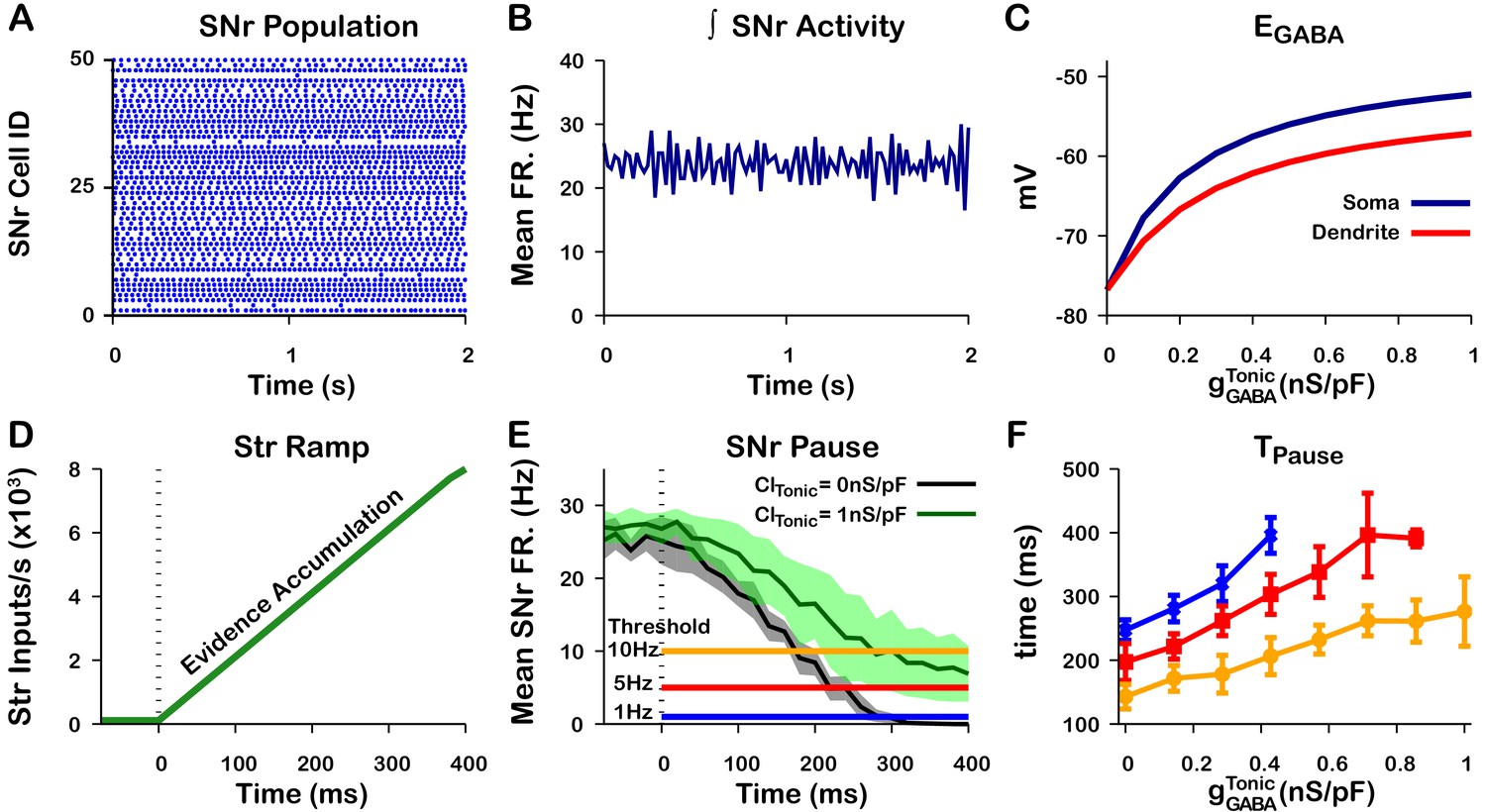
Tonic somatic conductance affects somatic and dendritic and tunes SNr responses to Str inputs.
(A) Raster plot of spikes in the simulation of an SNr network model containing 50 simulated neurons that receive tonic somatic inhibition from GPe projections. (B) Integrated SNr population activity gives a mean firing rate of about 23 Hz, as seen in in vivo conditions (Freeze et al., 2013; Mastro et al., 2017; Willard et al., 2019). (C) Increasing tonic depolarizes somatic and dendritic . (D) Ramping Str synaptic inputs used to represent evidence accumulation in a perceptual decision-making task. (E) Inhibition and pause generation in the SNr during evidence accumulation/ramping Str activity, for two different tonic somatic conductances. (F) Increasing the tonic conductance lengthens , the time for the SNr firing rate to drop below threshold (colors correspond to threshold levels in E). If the tonic conductance becomes too great, then SNr firing cannot be pushed to arbitrarily low rates. .
Figure 13—figure supplement 1
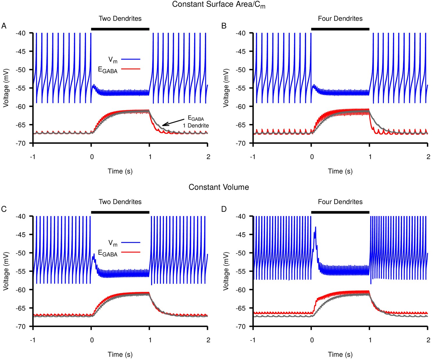
Switching from a single dendrite to multiple thin dendrites increases rate but not magnitude of accumulation and subsequent depolarization of in response to simulated Str stimulation.
Neuronal response (blue) and dynamics (red) in a neuron with (A,C) two or (B,D) four thin dendrites. For comparison dynamics in a neuron with a single dendrite is shown in gray in all panels. The total capacitance and surface area of the dendritic compartments in A and B matched that of the single dendrite; the total volume of the dendritic compartments in C and D matched that of the single dendrite. The stimulation period is from 0–1 s and is indicated by the horizontal black bar.
Figure 13—figure supplement 2
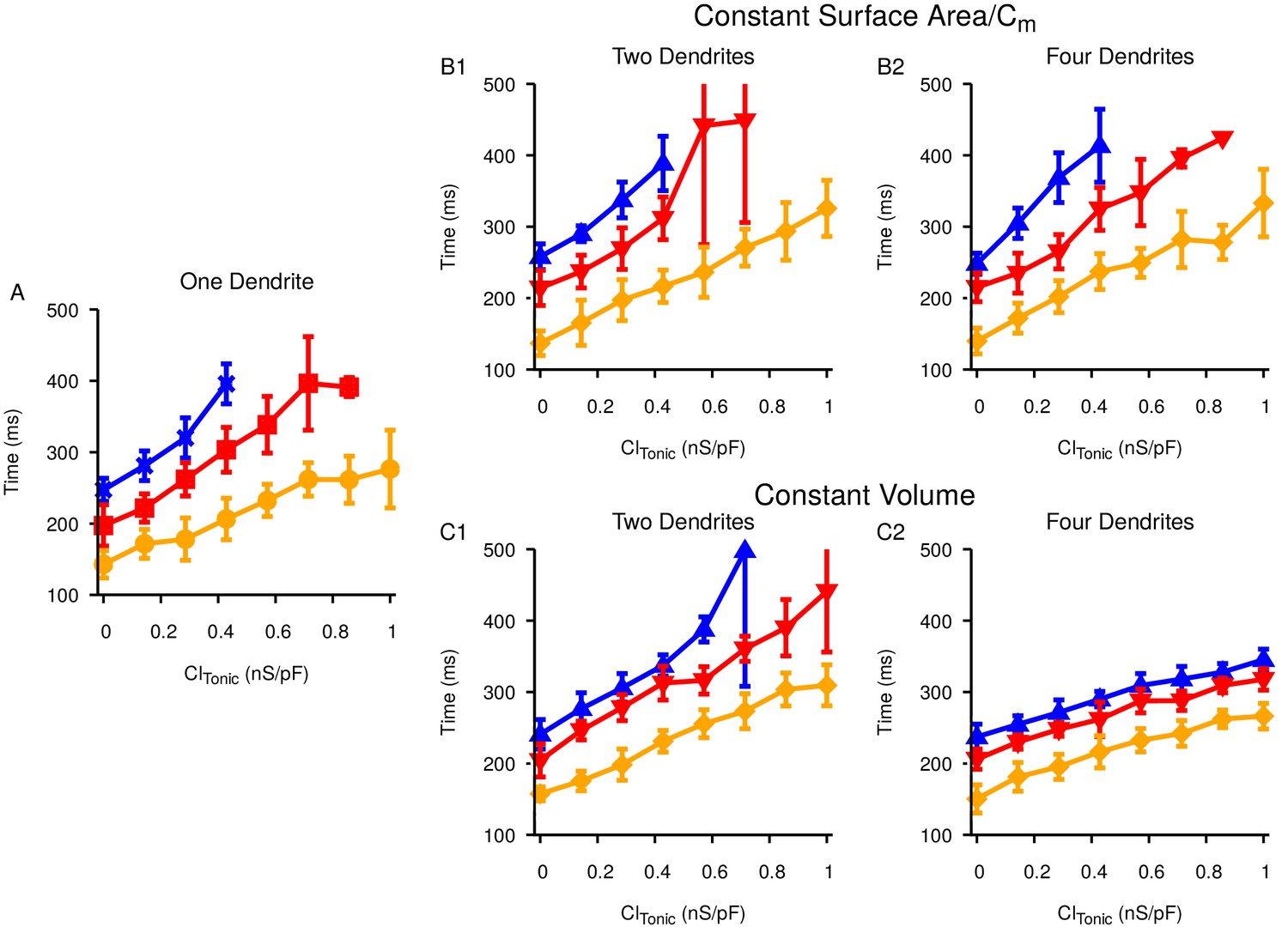
Increasing the number of dendrites has no qualitative effect on the the time it takes to generate a pause in SNr activity in response to ramping Str activity.
Relationship between the tonic conductance and for (A) one dendrite, (B) two (B1) or four (B2) dendrites with total surface area and capacitance matched to the single dendrite, and (C) two (C1) or four (C2) dendrites with total volume matched to the single dendrite. Colors correspond to three different pause thresholds, defined by SNr firing rates, as in Figure 11E in the main manuscript.
Figure 14

Summary figure/cartoon - GPe output provides tonic Cl load tuning SNr synchrony and the strength of Str inhibition.
Tables
Table 1
Ionic channel parameters.
| Channel | Parameters | ||
|---|---|---|---|
| IK | |||
| , see Equation 18 | |||
| , see Equation 23 | |||
| , | |||
| , see Equation 23 | |||
Additional files
Download links
A two-part list of links to download the article, or parts of the article, in various formats.
Downloads (link to download the article as PDF)
Open citations (links to open the citations from this article in various online reference manager services)
Cite this article (links to download the citations from this article in formats compatible with various reference manager tools)
The effects of chloride dynamics on substantia nigra pars reticulata responses to pallidal and striatal inputs
eLife 9:e55592.
https://doi.org/10.7554/eLife.55592


