Stochastic logistic models reproduce experimental time series of microbial communities
- Applied Physics Research Group, Physics Department, Vrije Universiteit Brussel, Belgium
- Interuniversity Institute of Bioinformatics in Brussels, Vrije Universiteit Brussel Université Libre de Bruxelles, Belgium
Figures
Figure 1
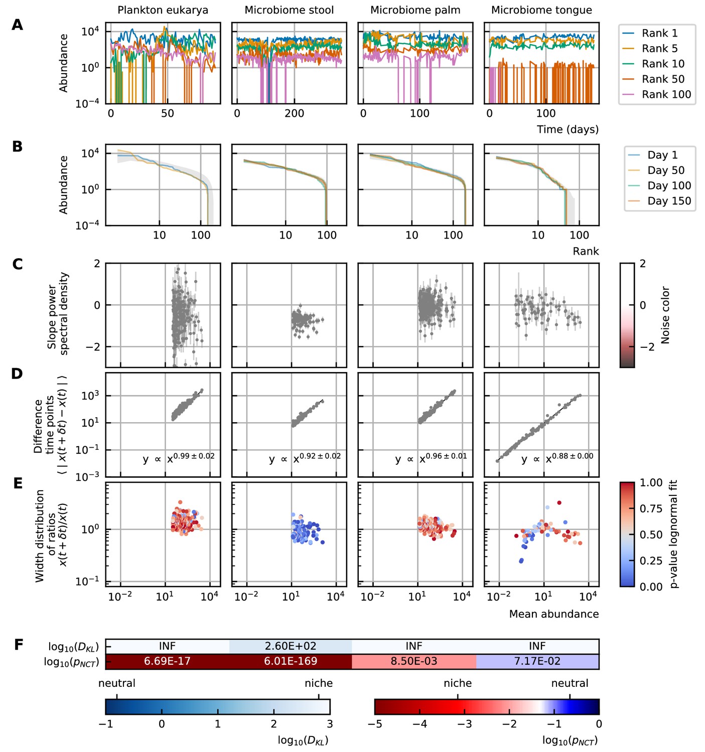
Characteristics of experimental data.
(A) Time series. (B) Rank abundance profile. The abundance distribution is heavy-tailed and the rank abundance remains stable over time. (C) Noise color: No clear correlation between the slope of the power spectral density and the mean abundance of the species can be seen. The noise colors corresponding to the slope of the power spectral density are shown in the colorbar (white, pink, brown, black). (D) Absolute difference between abundances at successive time points: There is a linear correspondence (in log-log scale) between the mean absolute difference between abundances at successive time points and the mean abundance of the species. Because the slope is almost one, this hints at the linear nature of the noise. (E) Width of the distribution of the ratios of abundances at successive time points: The width of the distribution of successive time points is large (order 1) and does not depend on the mean abundance of the species. Most of the species fit well a lognormal distribution: the p-values of the Kolmogorov-Smirnov test are high. (F) Neutrality: The values of the Kullback-Leibler divergence () and the neutral covariance test () are explicitly given. Additionally, we use color codes for both tests with the neutral regime represented by dark blue. White and red indicate the niche regime for the KL test and NCT respectively. We conclude that most experimental time series are in the niche regime.
Figure 2
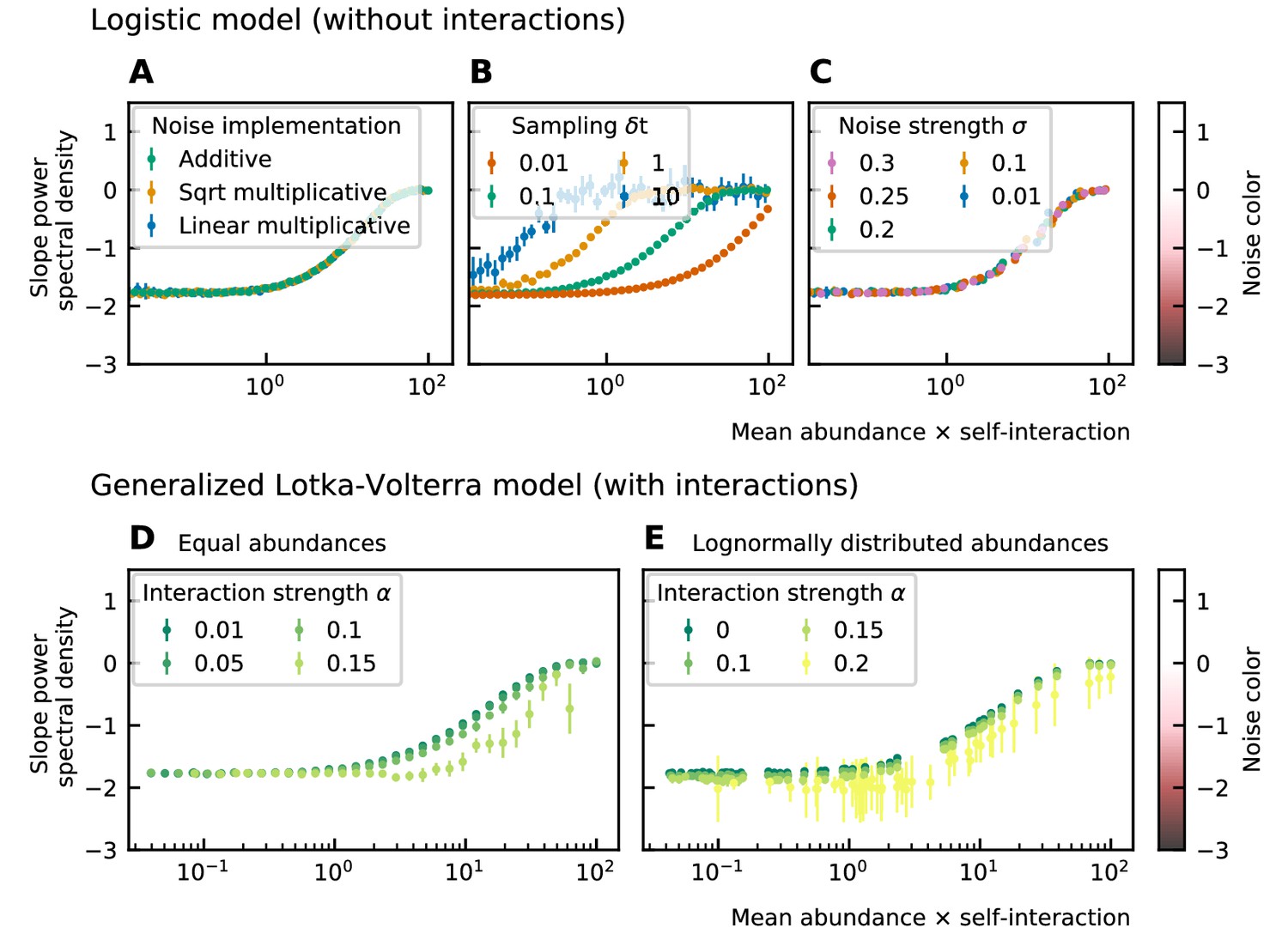
Noise color as a function of the mean abundance and self-interaction for stochastic logistic and gLV equations.
The noise colors corresponding to the slope of the power spectral density are shown in the colorbar (white, pink, brown, black). The mean abundance determines the noise color when there is no interaction, the implementation method (A) and the strength of the noise (C) have no influence. A smaller sampling time interval δt, which is equivalent to a higher sampling rate, makes the noise darker (B). For gLV models with interactions, larger interaction strengths make the noise colors darker for systems with equal abundances (D) as well as systems with heavy-tailed abundance distributions (E).
Figure 3
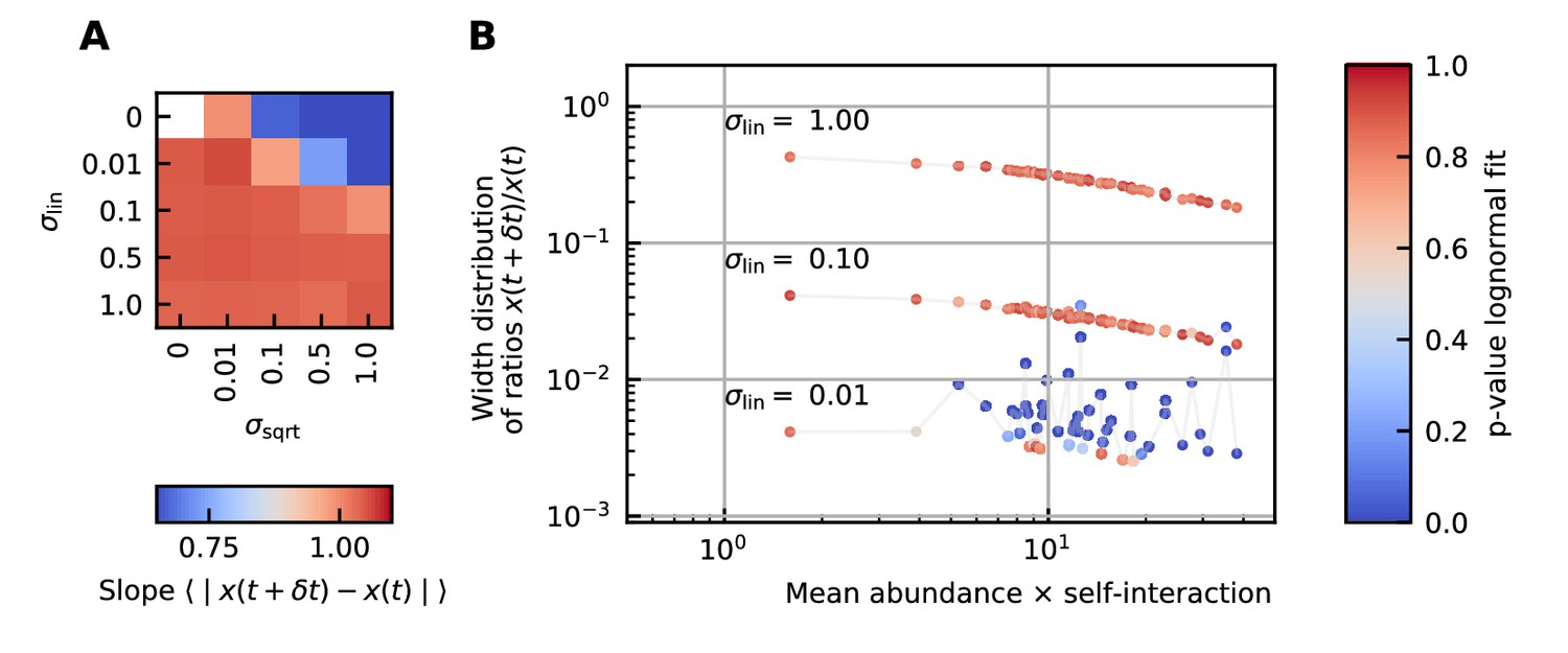
Differences between time points as a function of the noise.
(A) Correlation between the mean absolute differences between abundances at successive time points and the mean abundance for different strengths of the linear noise (σlin) and multiplicative noise that scales with the square root of the abundances (σsqrt). More specifically, the parameter represents the slope of the logarithm of the mean absolute difference between abundances at successive time points as a function of the logarithm of the mean abundance. Examples of such slopes are given by Figure 1D. Here, the slope ranges from 0.66 for noise that scales with the square root to one for linear noise. (B) The width of the distribution of the ratios of abundances at successive time points increases for increasing strength of the noise. For sufficiently strong noise the distribution is well fitted by a lognormal function (high p-values for the Kolmogorov-Smirnov test).
Figure 4

A stochastic logistic model is able to reproduce the different characteristics of the noise.
(A) Time series. (B) A rank abundance that remains stable over time. (C) Results of the neutrality test in the niche regime. (D) Noise color in the white-pink region with no dependence on the mean abundance. (E) The slope of the mean absolute difference between abundances at successive time points is around 1. (F) The width of the distribution of the ratios of abundances at successive time points is in the order of 1 and independent of the mean abundance.
Figure 5
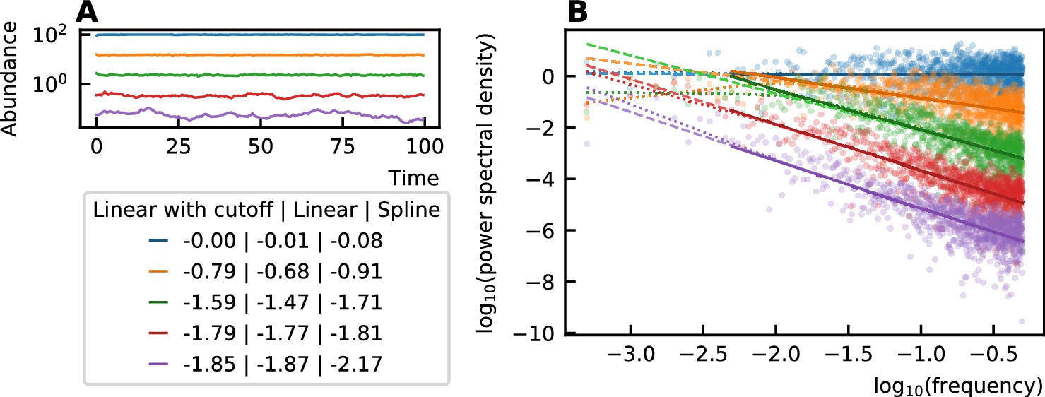
The noise color of time series (A) is determined by the slope of the power spectral density (B).
This slope can be measured through a linear fit of all values (dashed), a linear fit through the higher frequency range (solid line) or by performing a spline fit (dotted). A linear fit through all frequencies can be influenced by the windowing effect for low frequencies and the spline fit can make the slope steeper at the low frequencies and result in a darker noise as can be seen for the purple curves. The values of the noise color determined by the different techniques are given in the legend. Therefore, in our work, we opt for the linear fit with a cutoff for low frequencies.
Additional files
-
Supplementary file 1
Supplemental information.
Analysis of all experimental data. Rank abundance, distribution of the differences between abundance at successive time points, neutrality tests and noise color. Supporting results. Code All python codes to perform time series simulations, analysis and make all different figures of the main paper and supplement are available at https://github.com/lanadescheemaeker/logistic_models (Descheemaeker and de Buyl, 2020; copy archived at https://github.com/elifesciences-publications/logistic_models).
- https://cdn.elifesciences.org/articles/55650/elife-55650-supp1-v2.pdf
-
Transparent reporting form
- https://cdn.elifesciences.org/articles/55650/elife-55650-transrepform-v2.pdf
Download links
A two-part list of links to download the article, or parts of the article, in various formats.
Downloads (link to download the article as PDF and Executable version)
Open citations (links to open the citations from this article in various online reference manager services)
Cite this article (links to download the citations from this article in formats compatible with various reference manager tools)
Stochastic logistic models reproduce experimental time series of microbial communities
eLife 9:e55650.
https://doi.org/10.7554/eLife.55650


