Reinforcement regulates timing variability in thalamus
- Department of Bioengineering, University of Missouri, United States
- McGovern Institute for Brain Research, Department of Brain and Cognitive Sciences, Massachusetts Institute of Technology, United States
- Harvard-MIT Division of Health Sciences and Technology, United States
Figures
Figure 1
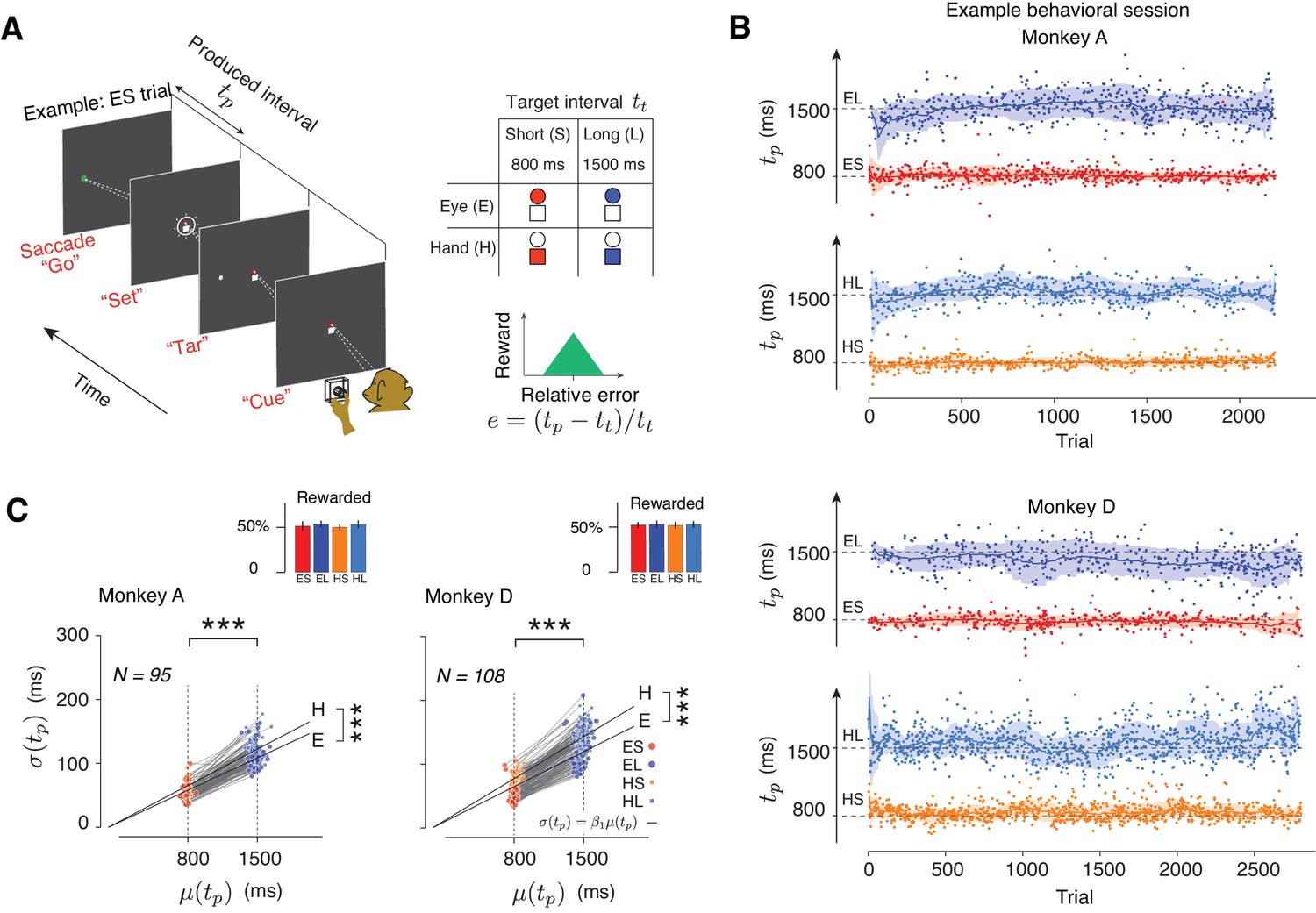
Task, behavior, and reward-dependency of variability.
(A) The Cue-Set-Go task. (B) Behavior in a representative session for each of the two animals. For visual clarity, tp values (dots) for different trial types are shown along different abscissae for each trial type. The solid line and shaded area are the mean and standard deviation of tp calculated from a 50-trial sliding window. (C) The standard deviation of tp (σ(tp)) as a function of its mean (μ(tp)) for each trial type in each behavioral session. Each pair of connected dots corresponds to Short and Long of the same effector in a single session. In both animals, the variability was significantly larger for the Long compared to the Short for both effectors (one-tailed paired-sample t test, ***p<<0.001, for monkey A, n = 190, t128 = 157.4; for monkey D, n = 216, t163 = 181.7). The solid black lines show the regression line relating σ(tp) to μ(tp) across all behavioral sessions for each trial type (σ(tp) = β1 μ(tp)). Regression slopes were positive and significantly different from zero for both effectors (β = 0.087 ± 0.02 mean±std for Eye and 0.096 ± 0.021 for Hand in Monkey A; β1 = 0.10 ± 0.02 for Eye and 0.12 ± 0.021 for Hand in Monkey D). Hand trials were more variable than Eye ones (one-tailed paired-sample t-test, for monkey A, n = 95, t52 = 6.92, ***p<<0.001, and for monkey D, n = 108, t61 = 6.51, ***p<<0.001). Inset: The overall percentage of rewarded trials across sessions for each trial type.
Figure 2 with 1 supplement
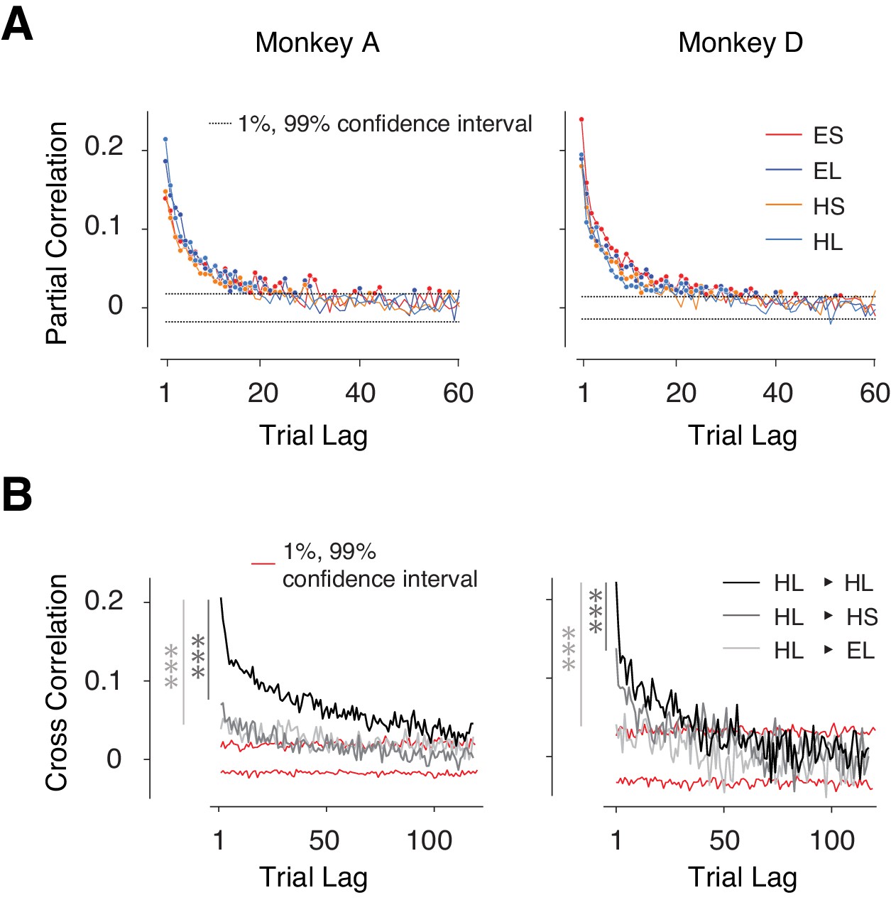
Context-dependent slow fluctuations of timing intervals.
(A) Long-term correlation of tp across trials of the same type (same effector and target interval). For each behavioral session, and each trial type, we computed the partial correlation of tp as a function of trial lag. Each curve shows the average partial correlations across all behavioral sessions. Four types of trials are shown in different colors. Filled circles: correlation values that are larger than the 1% and 99% confidence interval (dashed line). (B) Examples showing the Pearson correlation coefficients of tp's as a function of trial lag. HL-HL indicates the correlation was averaged across trials transitioning between HL and HL; 1% and 99% confidence intervals were estimated from the null distribution. Serial correlations were stronger between trials with the same effector and interval compared to trials with the same effector but different interval (*** dark gray, paired sample t-test on two sets of cross-correlations with less than 20 trial lags and combining four trial types; monkey A: p<<0.001, n = 80, t79 = 9.8; monkey D: p<<0.001, n = 80, t79 = 5.8), and trials of the different effector but same interval (*** light gray, monkey A: p<<0.001, n = 80, t79 = 6.7; monkey D: p<<0.001, n = 80, t79 = 17.3). See Figure 2—figure supplement 1A for transitions between other conditions, and Figure 2—figure supplement 1B for a comparison of context-specificity with respect to saccade direction.
Figure 2—figure supplement 1
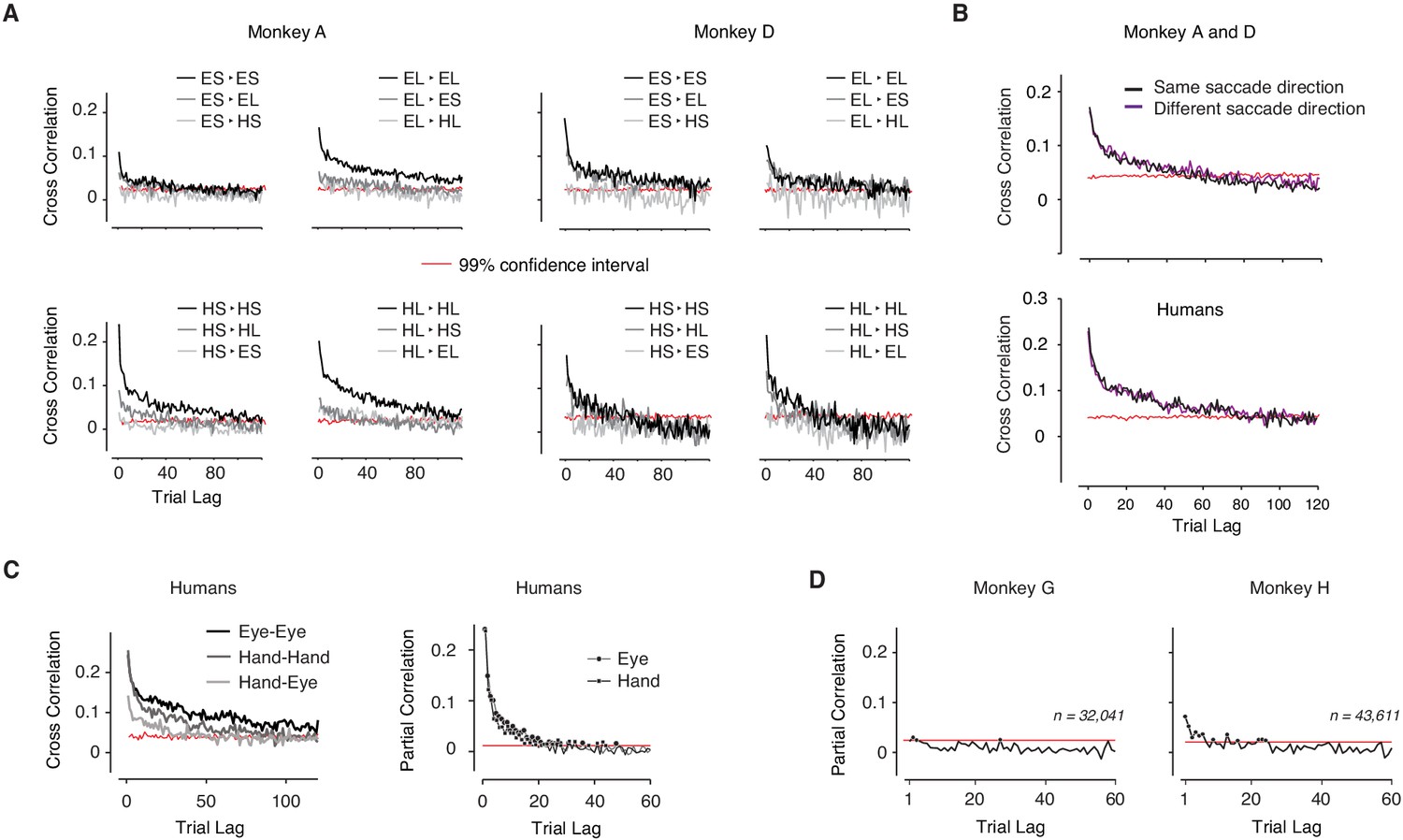
Slow fluctuations of timing variability.
(A) Correlation between produced intervals for the two animals and different trial types transitions. (B) Same as A between trials shown separately for trials with the same and different saccade directions (Top: monkeys; Bottom: humans). The analysis was performed separately for trials of the same type (i.e. same target interval and same effector), and pooled afterward. The long-term correlations were not significantly different for the same and different directions (Monkeys: paired sample t-test, p=0.39, t = 0.86, df = 159; Humans: paired sample t-test, p=0.55, t = 0.60, df = 79). (C) Slow fluctuations of timing variability in humans. Correlation was averaged across human subjects (N = 5). (D) Slow fluctuations of timing variability in the memory control experiment. Partial correlation between produced intervals diminished in the control experiment in which the demand for remembering the target interval was minimized. All plots are in the same format as in Figure 2. The red shows the high end of the 99% confidence intervals, which is approximated in each plot by averaging across bootstrap data across trials and conditions.
Figure 3 with 1 supplement
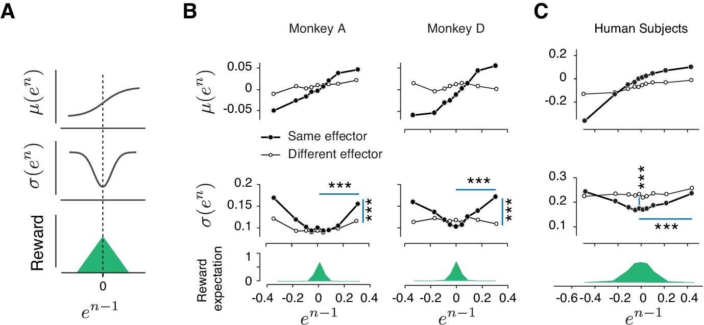
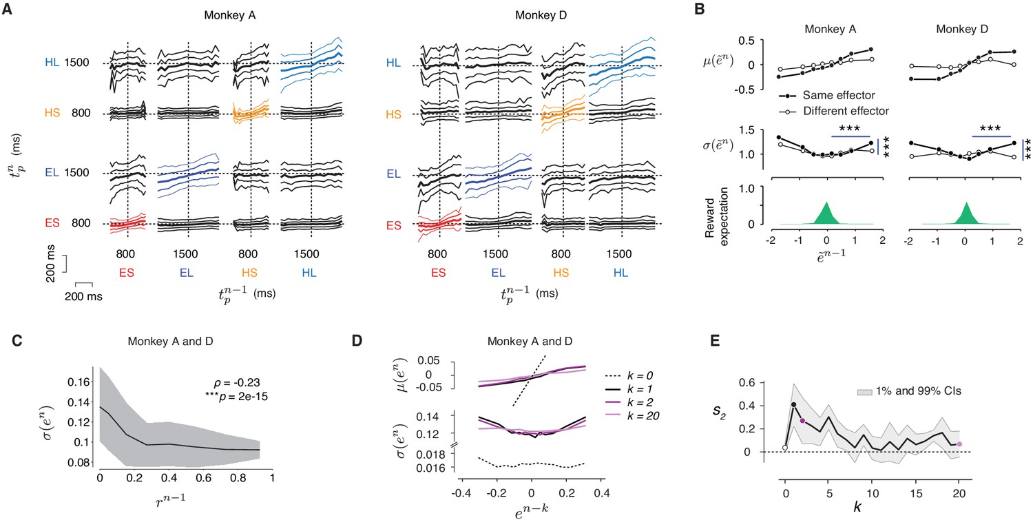
Rapid and context-dependent modulation of behavioral variability by reward.
(A) Illustration of the expected effect of serial correlations and reward-dependent variability. Top: Positive serial correlations between produced intervals (tp) creates a positive correlation between consecutive errors, and predicts a monotonic relationship between the mean of error in trial n, μ(en), and the value of error in trial n-1 (en-1). Middle: Variability decreases with reward. This predicts a U-shaped relationship between the standard deviation of en, σ(en), and en-1. Bottom: Reward as a function of en-1. (B) Trial-by-trial changes in the statistics of relative error. Top: μ(en) as a function of en-1 in the same format shown in (A) top panel. Filled and open circles correspond to consecutive trials of the same and different types, respectively. Middle: σ(en) as a function of en-1, sorted similarly to the top panel. Bottom: the reward expectation as a function of en-1. The reward expectation was computed by averaging the magnitude of reward received across trials. In the same effector, variability increased significantly after an unrewarded trials compared to a rewarded trials (horizontal line, two-sample F-test for equal variances, ***p<<0.001) for both large positive errors (Monkey A: F(11169,10512) = 1.09, Monkey D: F(18540,13478) = 1.76) and large negative errors (Monkey A: F(8771,9944) = 1.40, Monkey D: F(21773,14889) = 1.62). The variability after an unrewarded trial of the same effector was significantly larger than after an unrewarded trial of the other effector (vertical line, two-sample F-test for equal variances, ***p<<0.001) for both large positive errors (Monkey A: F(11169,8670) = 1.20, Monkey D: F(18540,7969) = 1.32) and large negative errors (Monkey A: F(8771,5994) = 1.26, Monkey D: F(21773,7179) = 1.27). (C) Same as (B) for human subjects. In humans, the variability was also significantly larger after a negatively reinforced trial compared to a positively reinforced trial (horizontal line, two-sample F-test for equal variances, ***p<<0.001) for both large positive errors (F(5536,5805) = 1.19) and large negative errors (F(9366,9444) = 1.11). The variability after a positively reinforced trial of the same effector was significantly lower than after a positively reinforced trial of the other effector (vertical line, two-sample F-test for equal variances, ***p<<0.001, F(14497,15250) = 1.10). For humans, the reward expectation was defined as the ratio between the number of trials with positive feedback and total number of trials.
Figure 3—figure supplement 1
The effect of reward on behavioral variability.
(A) Cross-condition relationship between produced interval (tp) in consecutive trials. The results for each animal are organized on a 4 × 4 panel covering the full set of 16 possible transitions between four trial types (ES: Eye-Short; EL: Eye-Long; HS: Hand-Short; HL: Hand-Long) with the abscissa and ordinate showing tp at trial n-1 (tpn-1) and n (tpn), respectively. In each panel, the median tpn as the function of tpn-1 is marked in bold at the center. The 25th and 75th percentile are marked with medium thickness, and the 10th and 90th percentile with thin lines. Bin size was 20 ms. (B) Error statistics across sessions. Since our original analysis was based on data combined across sessions, one potential concern we had was that modulation of tp variance with reward was due to differences across (but not within) sessions. To address this, we first removed outlier tp values (more than 3 s.d. away from the mean) and then analyzed z-scored errors within each session (denoted ). This normalization ensured that error pairs in every session were drawn from a zero-mean and unit-variance distribution. Results are shown in the same format as in Figure 3B–C. The variability increased significantly after unrewarded trials compared to that after rewarded trials (horizontal lines, ***p<0.001; monkey A: F(8889,10621) = 1.15 for negative and F(9841,11103) = 1.09 for positive ; monkey D: F(21216,12364) = 1.25 for negative and F(1600,19293) = 1.38 for positive ), and this effect was context specific (vertical lines, for monkey A: F(10621,9841) = 1.10 and monkey D: F(12364, 16100)=1.11). (C) Behavioral variability as a function of the magnitude of reward in the preceding trial. We computed σ(en) and the corresponding averaged reward rn-1 from randomly sampled trials without replacement within each bin of en-1. The dark line and shaded area showed the mean ±s.d. computed using a sliding window consisting of 50 samples. The σ(en) and reward rn-1 were significantly correlated (Spearman's ρ = −0.23, ***p<<1e-3). (D) Top: Average error on trial n, μ(en) as a function of error in trial n-k (en-k) for k = 0, 1, 2, and 20 (different colors). Bottom: Standard deviation of error on trial n, σ(en) as a function of en-k. Results were computed for each trial type separately averaged afterwards. (E) Modulation of variability by reward as a function of trial lag (k). Similar to the main paper, we tested the U-shaped profile using quadratic regression. The ordinate shows the coefficient of the square term (s2) of the quadratic regression as a function of trial lag (circles: s2 for the k values in D; shaded area: [1%–99%] confidence intervals). The reward has no direct bearing on the variability of the current trial (k = 0), and its effect drops as a function of trial lag.
Figure 4

Causal effect of reward on behavioral variability.
(A) Alternative interpretations of the relationship between the outcome of the preceding trial (Rewn-1) and behavioral variability in the current trial denoted σ(en). Left: A model in which Rewn-1causally controls σ(en). In this model, various factors (e.g.,memory drift) may determine the size of error (en-1), en-1 determines Rewn-1, and Rewn-1 directly regulates σ(en). Right: A model in which the relationship between Rewn-1 and σ(en) is correlational. In this model, Rewn-1 is determined by en-1, and σ(en) may be controlled by various factors (including en-1) but not directly by Rewn-1. (B,C) A time interval production task with probabilistic feedback to distinguish between the two models in (A). (B) Trial structure. The subject has to press the spacebar to initiate the trial. During the trial, the subject is asked to hold their gaze on a white fixation spot presented at the center of the screen. After a random delay, a visual ring (‘Set’) is flashed briefly around the fixation spot. The subject has to produce a time interval after Set using a delayed key press. After the keypress, the color of the fixation spot changes to red or green to provide the subject with feedback (green: ‘correct’, red: ‘incorrect’). (C) Top: A schematic illustration of the distribution of relative error , computed as (tp–tt)/tt. Bottom: After each trial, the feedback is determined probabilistically: the subject is given a ‘correct’ feedback with the probability of 0.7 when tp is within a window around tt, and with the probability of 0.3 when errors are outside this window. The window length was adjusted based on the overall behavioral variability so that each subject receives approximately 50% ‘correct’ feedback in each behavioral session. (D) The causal effect of the outcome of the preceding trial on behavioral variability in the current trial. Left: Scatter plot shows the behavioral variability after ‘incorrect’ (ordinate) versus ‘correct’ (abscissa) trials, for all five subjects, after trials in which en-1 was small (inset). Results for the positive and negative errors are shown separately (with ‘+’ and ‘-’ symbols, respectively). Right: Same as the left panel for trials in which en-1 was large (inset). In both panels, the variability across subjects was significantly larger following incorrect compared to correct trials (p<<0.001, paired sample t-test, t199 = 12.8 for small error, and t199 = 13.7 for large error, see Materials and methods).
Figure 5 with 2 supplements

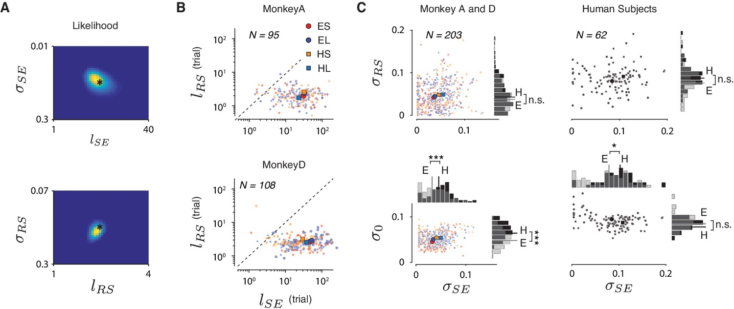
A reward-sensitive Gaussian process model (RSGP) capturing reward-dependent control of variability.
(A) Top: The covariance function for the RSGP model (KRSGP) is the sum of a squared exponential kernel (KSE), a reward-dependent squared exponential kernel (KRS) and an identity matrix (I) weighted by σSE2, σRS2, and σ02, respectively. Second row: Simulations of three GP models, one using KSE only (left), one using KRS only (middle), and one with the full KRSGP (right). Third row: Partial correlation of samples from the three GPs in the second row. Fourth and fifth rows: The relationship between the mean (fourth row) and standard deviation (fifth row) of en as a function of en-1 in the previous trial, shown in the same format as in Figure 3B. Only the model with full covariance function captures the observed behavioral characteristics. (B) Length scales, lSE and lRS associated with KES and KRS, respectively, derived from fits of RSGP to behavioral data from monkeys (left) and humans (right). Small and large symbols correspond to individual sessions and the median across sessions, respectively. Different trial types are shown with different colors (same color convention as in Figure 1B). lRS was significantly smaller than the lSE (monkeys: p<<0.001, one-way ANOVA, F1, 945 = 463.4; humans: p<<0.001, one-way ANOVA, F1, 235 = 102.5). (C) Statistics of the predicted behavior from the RSGP model fits, shown in the same format as Figure 3B,C. Data were generated from forward prediction of the RSGP model fitted to behavior (see Materials and methods for details). The standard error of the mean computed from n = 100 repeats of sampling of trials is shown as a shaded area, but it is small and difficult to discern visually.
Figure 5—figure supplement 1
RSGP model fits.
(A) Simulation results indicated that the likelihood function captures the ground truth and that the error surface is convex for a wide range of initial values. See Materials and methods for details. The hyperparameters used for simulation are marked by asterisks and the results of fitting are in Table 2. (B) Same as Figure 5B shown for the two animals separately. (C) The model fit of variances (σSE, σRS and σ0) across sessions for monkeys (left column) and humans (right column).
Figure 5—figure supplement 2
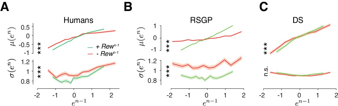
Analysis of error statistics in the probabilistic reward experiment.
(A) Human behavior. Results were combined for all subjects in Figure 4D and was plotted in the same format as Figure 3B. To avoid sampling bias, same number of trials were drawn repeatedly after ‘incorrect’ (red, –Rewn-1) or ‘correct’ (green, +Rewn-1) trials (Shaded area: standard error of the mean computed from 100 bootstraps). Behavioral variability σ(en) increased significantly after ‘incorrect’ trial outcome regardless of the size of error (***p<0.001, two-sample t-test on σ(en) between the two conditions, t198 >6.70 for all bins). The slope of the μ(en) as a function of en-1 was larger after ‘correct’ outcome (***p<0.001, two sample t-test t198 = 16.8) demonstrating stronger behavioral correlation after positive reinforcement. (B) RSGP model behavior. Same as (A) for the behavior of the RSGP model fit to the subject’s behavior. (C) DS model behavior. Same as (B) for the model fit to the subject’s behavior (slope of the μ(en), ***p<0.001, two sample t-test t198 = 5.11, larger σ(en) after ‘incorrect’: one-sided two-sample t-test, p>=0.85).
Figure 6 with 1 supplement
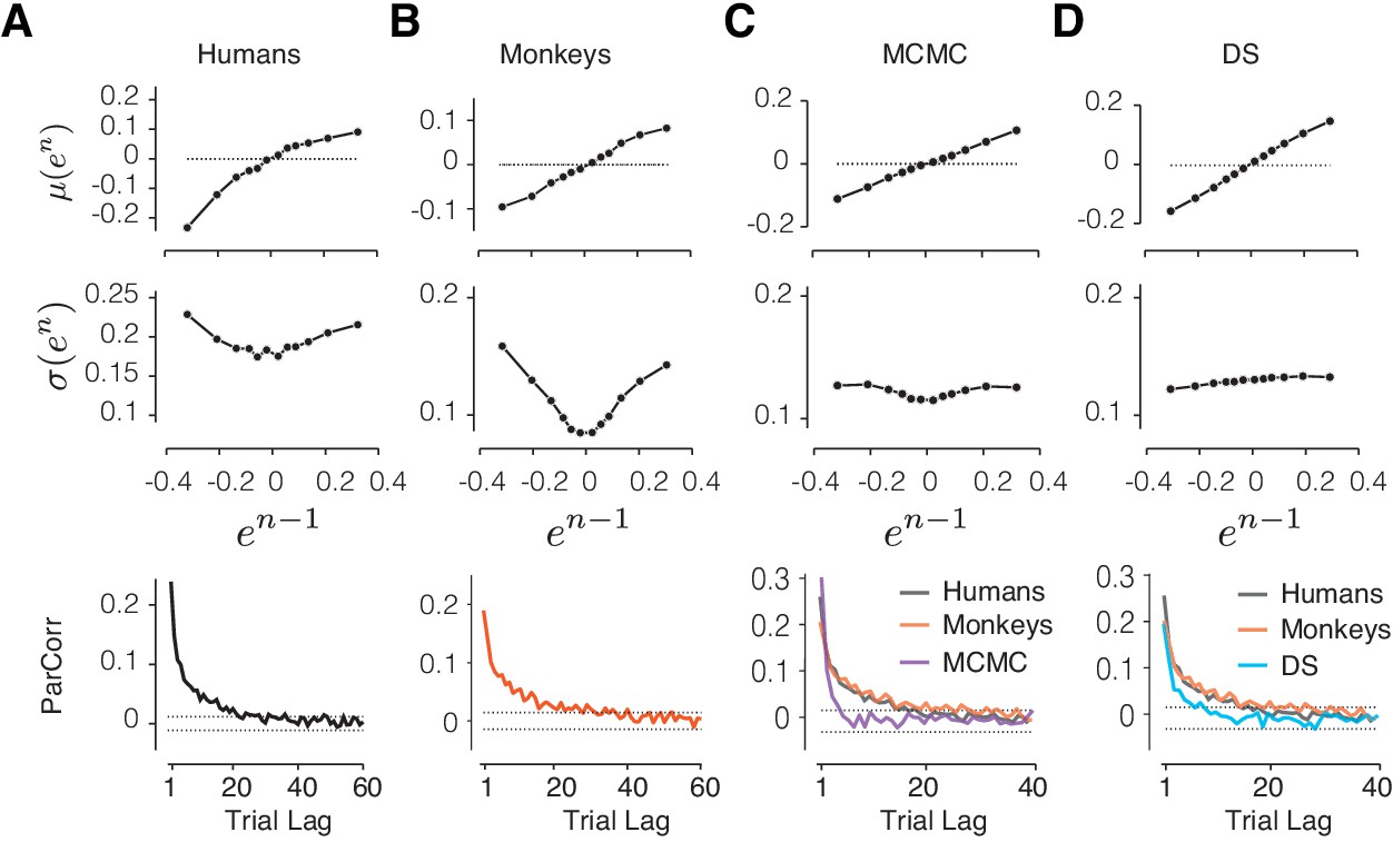
Comparison of alternative models to behavioral data and the RSGP model.
(A) Human behavior. Top: Same results as Figure 3 showing the monotonic relationship between the mean of error in trial n, μ(en), and the value of error in trial n-1 (en-1). Middle: Same as Figure 3 showing the U-shaped relationship between the standard deviation of en, σ(en), and en-1. Bottom: Same as Figure 2A showing partial correlation between produced intervals. (B) Same as (A) for data pooled across the animals. (C) Same as (A) for simulations of the RL-based Markov chain Monte Carlo (MCMC) sampling model. The data for humans and monkeys are included in the bottom panel for comparison. (D) Same as (C) for the RL-based directed search (DS) model based on the subset of simulation that did not exhibit run-away behavior.
Figure 6—figure supplement 1
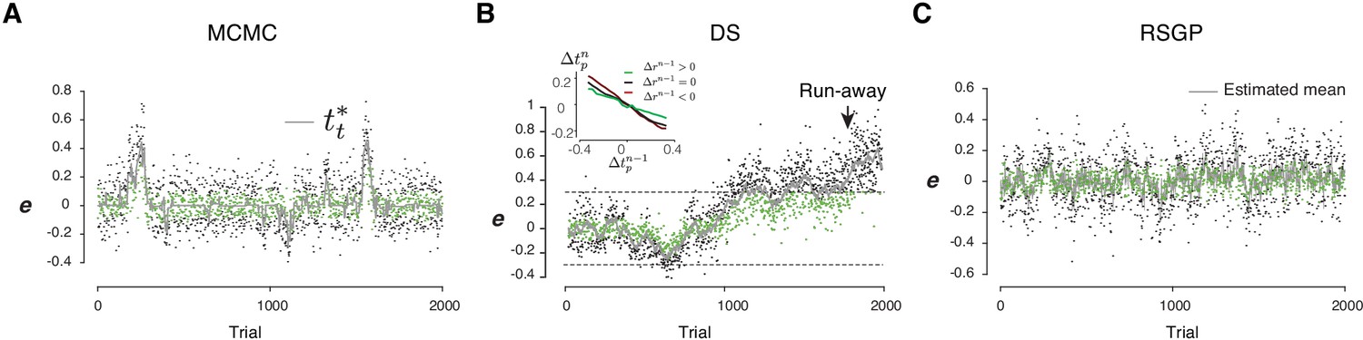
Example RL-based model behavior.
(A) An example simulation of the RL-based Markov chain Monte Carlo (MCMC) sampling model with parameters fitted to the animals’ behavior. tt* is the internal target associated with the highest value. Rewarded trials were in green and unrewarded ones were in black. (B) Same as (A) for the RL-based directed search (DS) model. Inset: The mean of Δtpn as a function of Δtpn-1 for different values of Δrn-1. The positive and negative reward gradient has the opposite effect on the relationship. The overall negative correlation between Δtpn and Δtpn-1 is due to the classic regression to the mean. (C) Same as (A) for the RSGP model. Each point reflects the trial-by-trial updated posterior mean.
Figure 7
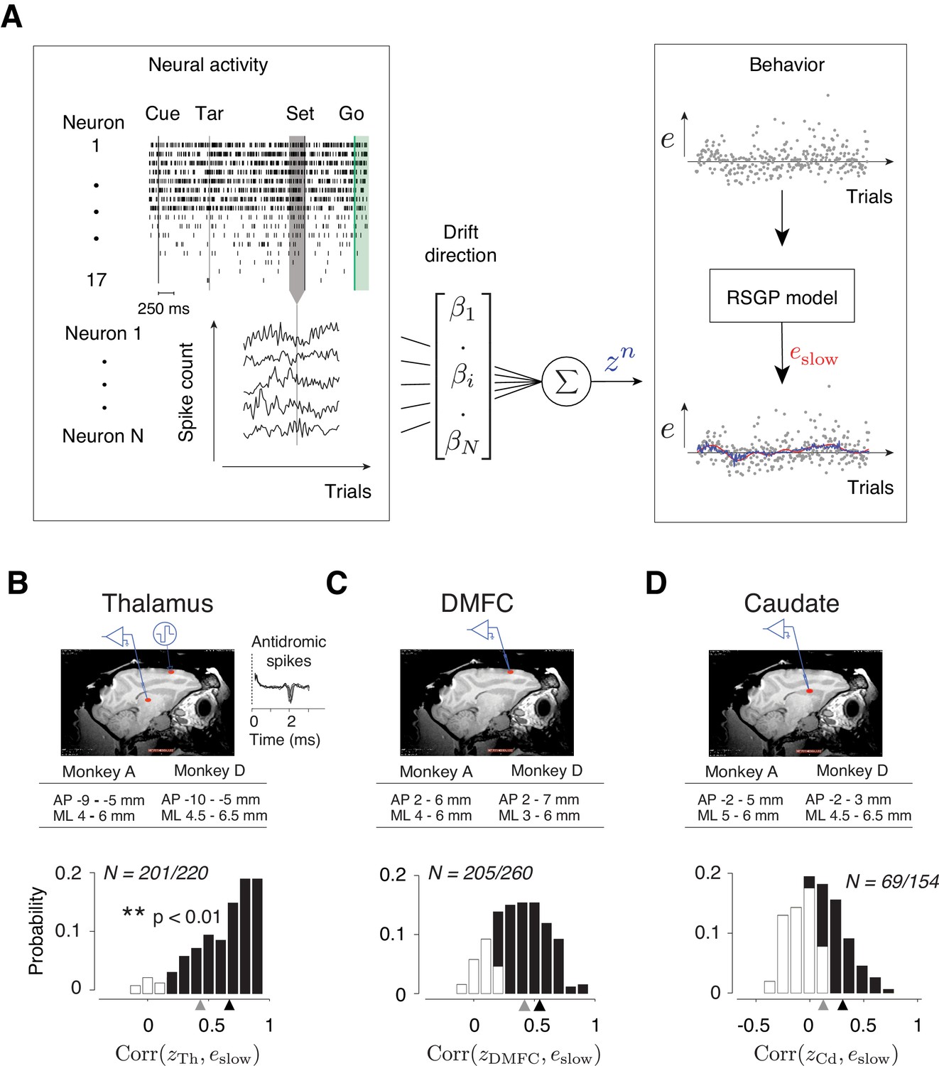
Representation of slow fluctuations of behavior in population activity.
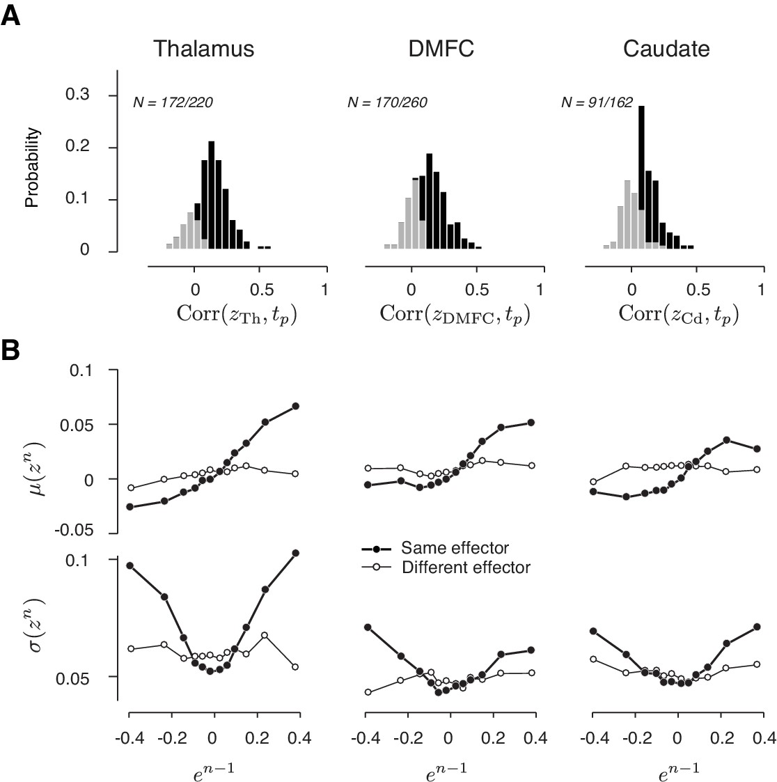
(A) The schematics of the analysis for identifying the drift direction across a population of simultaneously recorded neurons. Top left: The rows show spike times (ticks) of 17 simultaneously recorded thalamic neurons in an example trial. From each trial, we measured spike counts within a 250 ms window before Set (gray region). Bottom left: The vector of spike counts from each trial (gray vertical line) was combined providing a matrix containing the spike counts of all neurons across all trials. Middle: The spike counts across trials and neurons were used as the regressor in a multi-dimensional linear regression model with weight vector, β, to predict the slow component of error (eslow). Right: We fitted the RSGP to errors (black dots, e) and then inferred eslow. The plot shows the neural prediction (zn, blue) overlaid on eslow derived from RSGP fit to behavior (red line). (B) Top: Parasagittal view of one of the animals (monkey D) with a red ellipse showing the regions targeted for electrophysiology. The corresponding stereotactic coordinates relative to the anterior commissure in each animal (AP: anterior posterior; ML: mediolateral). Recorded thalamic neurons were from a region of the thalamus with monosynaptic connections to DMFC (inset: antidromically activated spikes in the thalamus.) Bottom: Histogram of the correlation coefficients between eslow inferred from the RSGP model and znTh (projection of thalamic population activity on drift direction) across recording sessions. Note that some correlations are negative because of cross-validation. Black bars correspond to the sessions in which the correlation was significantly positive (**p<0.01; hypothesis test by shuffling trial orders). The average correlation across all sessions and the average of those with significantly positive correlations are shown by gray and black triangles, respectively. (C) Same as B for DMFC. (D) Same as B for the caudate.
Figure 8 with 6 supplements
Alignment of reward-dependent neural variability and drift in thalamus, but not in DMFC and caudate.
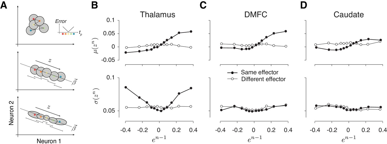
(A) Various hypotheses for how population neural activity could be related to produced intervals (tp) shown schematically in two dimensions (two neurons). Top: The average neural activity (colored circles) is not systematically organized with respect to tp, and the trial-by-trial variability of spike counts for a given tp around the mean (gray area) is not modulated by the size of the error. The inset shows how error increases as tp moves away from the target interval (tt). Middle: Projection of average activity along a specific dimension (dotted line) is systematically ordered with respect to tp, but the variability (small stacked arrows) does not depend on the size of the error. Bottom: Projection of average activity along a specific dimension is systematically ordered with respect to tp and the variability along the same axis increases with the size of error. (B) The relationship between neural activity in the thalamus on trial n and relative error in the preceding trial (en-1). Top: Expected mean of population activity on trial n (μ(zn)) along the drift direction (β) as a function of en-1. Bottom: Expected standard deviation of population activity along the drift direction on trial n (σ(zn)) as a function of en-1. Results are shown in the same format as in Figure 3B (thick lines: same effector; thin lines: different effectors). (C) and (D) Same as (B) for population activity in DMFC and caudate. See Figure 8—figure supplement 1 for the result of individual animals. The results in panels B-D were based on spike counts in a fixed 250-ms time window before Set. Figure 8—figure supplement 4 shows that these characteristics were evident throughout the trial. Figure 8 and Figure 8—figure supplement 5 show the effects for each effector and that the effect for different effectors were associated with different patterns of activity across the same population of neurons.
Figure 8—figure supplement 1
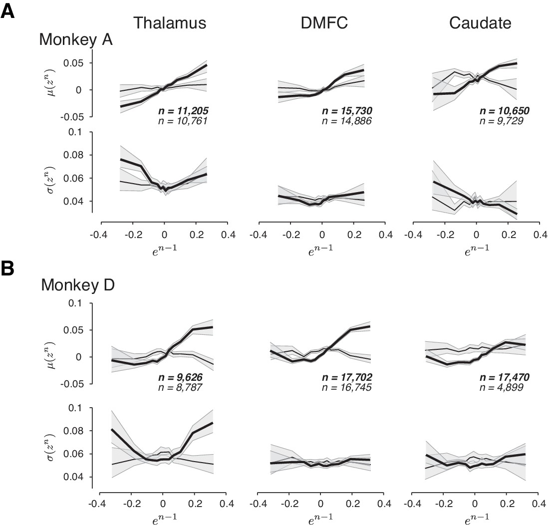
The relationship between neural activity on trial n to relative error in the preceding trial (en-1) in three brain areas and two animals.
(A) and (B) Same format as in Figure 8B–D, with the addition of confidence intervals (1–99%; shaded region) obtained by randomly sampling a subset of trials in each bin of en-1. Data shown for the two animals separately.
Figure 8—figure supplement 2
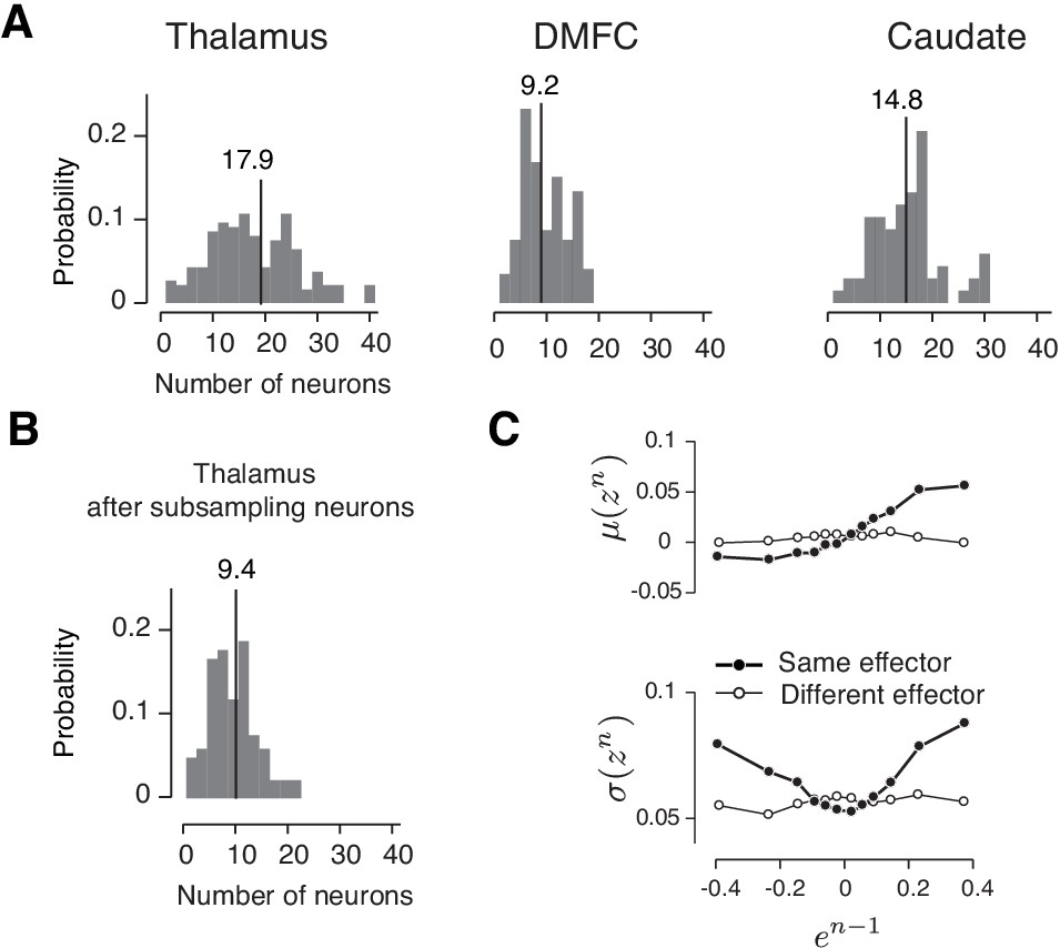
Drift and reward-dependent variability in the three brain areas inferred from comparable numbers of simultaneously recorded neurons.
(A) Histogram of the number of simultaneously recorded neurons in the thalamus, DMFC and caudate across sessions. The averages are shown on top. (B) The number of simultaneously recorded neurons in the thalamus subsampled by a factor of 2 to approximately match DMFC. (C) Analysis of drift and reward-dependent variability for the sub-sampled thalamic population, shown in the same format as Figure 8B.
Figure 8—figure supplement 3
Drift and variability of spike count along the direction that decodes the produced interval (tp) in the thalamus, DMFC, and caudate.
(A) Histogram of the correlation coefficients between tp and the output of a decoder of tp from neural data, denoted z (black: significantly positive). Results are shown with the same format as in Figure 7B. (B) Mean (top; μ(zn)) and standard deviation (bottom; σ(zn)) of projected neural activity as a function of error in the preceding trial (en-1). Results are shown with the same format as in Figure 8B (thick lines: same effector; thin lines: different effectors).
Figure 8—figure supplement 4
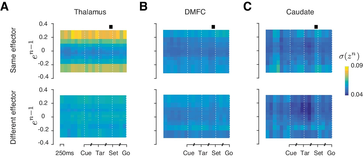
Reward-dependent neural variability throughout the trial.
(A) Average standard deviation of population activity in the thalamus at different points throughout the trial aligned to the Cue, Tar, Set, and Go events. For each time point, we inferred the drift direction using the same analysis shown in Figure 7A, and projected spike counts onto the drift direction. We denote the projection of trial n by zn. Each column shows the standard deviation of zn (σ(zn)) as a function of error in the preceding trial (en-1) based on spike counts within a 250-ms window centered at a particular time point in the trial. Black square: the time window used for the rest of this paper. We grouped en-1 into 12 bins, 6 for negative en-1 and 6 for positive en-1. Results are shown separately for conditions in which trials n-1 and n were of the same or different effectors. (***p<0.001, using a two-sample F-test comparing the variance of zn between rewarded and unrewarded trials separately for positive and negative values of en-1; H0: equal variance for at least one of the comparisons). (B) and (C) Same as (A) for DMFC and caudate. Results are for data combined across two animals.
Figure 8—figure supplement 5
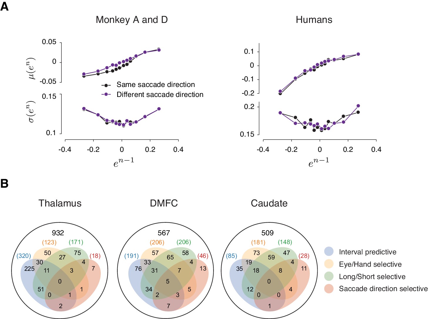
Analysis of neural data in relation to saccade direction.
(A) Error statistics across consecutive trials. μ(en) (top) and σ(en) (bottom) as a function of en-1. Similar to the main paper, we tested the U-shaped profile using quadratic regression. The coefficients of the squared term was not significantly different between the two directions (Monkeys: 0.26 [0.17, 0.34] vs 0.27 [0.2, 0.34]; Humans: 0.33 [0.063, 0.59] vs 0.4 [0.24, 0.55]). (B) A Venn diagram showing the number of individual neurons in three brain areas whose spiking during a 250 ms time window before Set was significantly different across effectors (Eye/Hand; p<0.01, two-sample t-test), target intervals (Short/Long; p<0.01, two-sample t-test), saccade directions (Left/Right; p<0.01, two-sample t-test), and predictive of the produced interval (p<0.01, shuffling test). The number of neurons in each category is indicated in the diagram. Among the neurons that were predictive of the produced interval (intersection of blue and dark red), 3/320 in the thalamus, 17/191 in DMFC, and 1/85 in the caudate were direction selective.
Figure 8—figure supplement 6
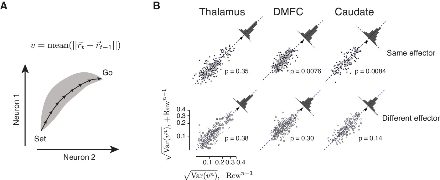
Analysis of speed variability across single trials as a function of reward.
(A) Schematics showing how we estimated the speed of population neural trajectories for single trials (vn). We estimated the average speed for each trial by averaging the Euclidean distance of population spike counts between nearby points (dt = 125 ms) along the trajectory. To minimize the differential contribution of neurons with different average firing rates to speed estimates, spike counts for each neuron was normalized (z-score) across trials and time bins. (B) Variability of speed estimates () after rewarded trials (+Rewn-1, ordinate) compared to unrewarded trials (-Rewn-1, abscissa) for consecutive trials of the same (top row) and different effector (bottom row) in the thalamus (left), DMFC (middle) and caudate (right). In every session, each trial type contributed two points to each panel, one for when the preceding error was positive and one for when it was negative. We treated these two error conditions independently so as to minimize any potential dependence of our estimated on average speed vn that may change depending on the sign of error (Wang et al., 2018). The scatter plot in each panel shows the distribution of speed variability for trials that succeeded a rewarded trial (ordinate) relative to the distribution of speed variability for trials that succeeded an unrewarded trial (abscissa). To test whether the speed was significantly different between these two conditions, we used a two-tail paired sample t-test to determine whether and in which direction the data deviated significantly from the unity line (diagonal). The distribution of the difference between the two conditions is shown on the top right of each panel, and the mean for each distribution is indicated (triangle). p-Values for each test are indicated. (Thalamus: same effector, t271 = 0.94, different effector, t271 = −0.88, DMFC: same effector, t313 = 2.69, different effector, t313 = 1.03, Caudate: same effector, t161 = 2.67, different effector, t161 = 1.47).
Tables
Table 1
Quantitative assessment of the dependence of μ(en) and σ(en) on en-1.
| Parameters | Monkey A | Monkey D | Humans |
|---|---|---|---|
| Same vs. different effector | Same vs. different effector | Same vs. different effector | |
| m1 m0 | 0.16 [0.12, 0.19]>0.04 [0.03, 0.06] 0.00 [-0.00, 0.01]~0.01 [0.01, 0.01] | 0.20 [0.12, 0.28]>−0.00 [-0.05, 0.04] −0.00 [-0.02, 0.01]~0.01 [0.00, 0.02] | 0.35 [0.27, 0.44]>0.15 [0.09, 0.20] −0.03 [-0.08, 0.02]~−0.06 [-0.08,–0.05] |
| s2 s1 s0 | 0.50 [0.39, 0.60]>0.24 [0.14, 0.33] −0.02 [-0.04, 0.01]~0.02 [-0.00, 0.04] 0.09 [0.09, 0.10]~0.08 [0.08, 0.92] | 0.48 [0.19, 0.78]>−0.06 [-0.17, 0.05] 0.03 [-0.03, 0.10]~−0.01 [-0.04, 0.01] 0.11 [0.10, 0.12]~0.12 [0.11, 0.12] | 0.31 [0.21, 0.42]>0.06 [-0.03, 0.16] 0.00 [-0.03, 0.04]~0.03 [-0.00, 0.06] 0.17 [0.16, 0.19]<0.22 [0.22, 0.24] |
Table 2
Ground truth versus model fits for the hyperparameters used in RSGP simulation in Figure 5A and Figure 5—figure supplement 1A.
| Ground truth | 20.0 | 0.141 | 2.0 | 0.141 | 0.10 |
| MML fit | 18.4 | 0.129 | 2.14 | 0.137 | 0.0749 |
Table 3
Regression model fits relating spike count along the drift direction on trial n (zn) to error in trial n-1 (en-1).
m0 and m1 are parameters of the linear regression model relating the mean of zn (μ(zn)) to en-1, that is, μ(zn) = m0+m1en-1. s0, s1 and s2 are parameters of the quadratic regression model relating the standard deviation of zn (σ(zn)) to en-1, that is, σ(zn) = s0+s1en-1+s2(en-1)2. Fit parameters are shown separately for the thalamus, DMFC and caudate and further separated depending on whether trial n-1 and n were of the same or different effectors. Bold values for m1 and s2 were significantly positive (** p<0.01, 1% and 99% confidence intervals of the estimation were shown).
| Brain area | Parameters | Same effector | Different effector | |
|---|---|---|---|---|
| Thalamus | μ(zn) | m1 m0 | 0.13 [0.090 0.18] 0.008 [0.001 0.016] | 0.0038 [-0.025 0.032] 0.0041 [-0.001 0.009] |
| σ(zn) | s2 s1 s0 | 0.26 [0.19 0.34] 0.005 [-0.013 0.023] 0.06 [0.052 0.059] | 0.0031 [-0.031 0.037] −0.001 [-0.01 0.0067] 0.058 [0.057 0.0597] | |
| DMFC | μ(zn) | m1 m0 | 0.11 [0.0334 0.18] 0.012 [-0.0003 0.024] | −0.0027 [-0.022 0.017] 0.0069 [0.0036 0.01] |
| σ(zn) | s2 s1 s0 | 0.071 [-0.003 0.12] 0.0085 [-0.0022 0.019] 0.046 [0.044 0.048] | 0.0051 [-0.037 0.047] −0.0004 [-0.01 0.009] 0.0487 [0.047 0.051] | |
| Caudate | μ(zn) | m1 m0 | 0.068 [0.016 0.12] 0.0068 [-0.002 0.015] | 0.007 [-0.016 0.030] 0.018 [0.014 0.022] |
| σ(zn) | s2 s1 s0 | 0.069 [-0.005 0.14] 0.0006 [-0.009 0.011] 0.048 [0.046 0.050] | −0.002 [-0.064 0.060] 0.001 [-0.013 0.015] 0.048 [0.045 0.051] | |
Table 4
Regression model fits relating spike count along the direction that predicts produced interval (tp) on trial n (zn) to error in trial n-1 (en-1).
m0 and m1 are parameters of the linear regression model relating the mean of zn (μ(zn)) to en-1; i.e., μ(zn) = m0+m1en-1. s0, s1 and s2 are parameters of the quadratic regression model relating the standard deviation of zn (σ(zn)) to en-1; i.e., σ(zn) = s0+s1en-1+s2(en-1)2. Fit parameters are shown separately for the thalamus, DMFC and caudate and further separated depending on whether trial n-1 and n were of the same or different effectors. Bold indicated significantly positive value (p<0.01, 1% and 99% confidence intervals of the estimation were shown).
| Brain area | Parameters | Same effector | Different effector | |
|---|---|---|---|---|
| Thalamus | μ(zn) | m1 m0 | 0.13 [0.096 0.17] 0.012 [0.005 0.019] | 0.018 [0.002 0.036] 0.006 [0.002 0.01] |
| σ(zn) | s2 s1 s0 | 0.32 [0.19 0.44] 0.012 [-0.019 0.046] 0.063 [0.055 0.071] | −0.019 [-0.07 0.066] −0.003 [-0.02 0.014] 0.065 [0.061 0.069] | |
| DMFC | μ(zn) | m1 m0 | 0.091 [0.043 0.14] 0.014 [0.0046 0.024] | 0.011 [-0.0073 0.29] 0.011 [0.0075 0.015] |
| σ(zn) | s2 s1 s0 | 0.15 [0.087 0.21] −0.006 [-0.022 0.009] 0.049 [0.045 0.052] | −0.017 [-0.071 0.036] 0.001 [-0.0041 0.024] 0.051 [0.047 0.054] | |
| Caudate | μ(zn) | m1 m0 | 0.077 [0.036 0.12] 0.010 [0.0014 0.018] | 0.007 [-0.012 0.027] 0.015 [0.011 0.019] |
| σ(zn) | s2 s1 s0 | 0.16 [0.11 0.21] 0.005 [-0.007 0.17] 0.050 [0.047 0.053] | 0.044 [0.016 0.072] −0.0025 [-0.01 0.0047] 0.051 [0.049 0.053] | |
Table 5
Algorithm for generating time series based on RSGP model.
| for n = 1...N do 1. Given the previous value and reward history, infer the mean and The variance of tpn from the conditional distribution 2. Randomly sample tpn from the inferred mean and variance 3. Update the reward-sensitive covariance, KRS, and the full kernel, KRSGP, based on tpn. end |
Table 6
Algorithm for generating time series based on MCMC model.
| for each trial do 1. Keep an internal estimate of target tt* that is currently associated with the highest reward, V(tt*). 2. On every trial, sample a new target, denoted tt+, from a Gaussian distribution with mean tt* and standard deviation We. 3. Generate tp by sampling from a Gaussian distribution with mean tt+ and standard deviation tt+. Wp (scalar noise). Assign the reward as the value of new sample V(tt+). 4. Use a probabilistic Metropolis-Hastings rule to accept or reject tt+ as the new target depending on the relative values of V(tt+), V(tt*), and a free parameter β known in RL as the inverse temperature. end |
Table 7
Algorithm for simulating the DS model.
| for n = 1...N do 1. Generate a new target estimation ttn using gradients derived from the previous performance and reward Δtt = α (ttn-1 - ttn-2) * (rn-1 - rn-2) ttn = ttn-1 + Δtt + ne, in which the estimation noise ne ~ N(0,We) 2. Generate tpn with the added scalar production noise ~ N(0,Wp) 3. Compute the amplitude of reward rn based on tpn and reward profile end |
Additional files
Download links
A two-part list of links to download the article, or parts of the article, in various formats.
Downloads (link to download the article as PDF)
Open citations (links to open the citations from this article in various online reference manager services)
Cite this article (links to download the citations from this article in formats compatible with various reference manager tools)
Reinforcement regulates timing variability in thalamus
eLife 9:e55872.
https://doi.org/10.7554/eLife.55872


