Recent shifts in the genomic ancestry of Mexican Americans may alter the genetic architecture of biomedical traits
- Biomedical Sciences Graduate Program, University of California, San Francisco, United States
- Department of Bioengineering and Therapeutic Sciences, University of California, San Francisco, United States
- McGill Genome Centre, McGill University, Canada
- Department of Human Genetics, McGill University, Canada
- Quantitative Life Sciences Program, McGill University, Canada
- Division of General Internal Medicine, University of California, San Francisco, United States
- Department of Medicine, University of California, San Francisco, United States
- Institute of Human Genetics, University of California, San Francisco, United States
- Helen Diller Family Comprehensive Cancer Center, University of California, San Francisco, United States
- Native BioData Consortium, United States
- Bloomberg School of Public Health, Johns Hopkins University, United States
- Department of Epidemiology and Biostatistics University of California, San Francisco, United States
- Bakar Computational Health Sciences Institute, University of California, San Francisco, United States
- Quantitative Biosciences Institute, University of California, San Francisco, United States
Figures
Figure 1 with 1 supplement
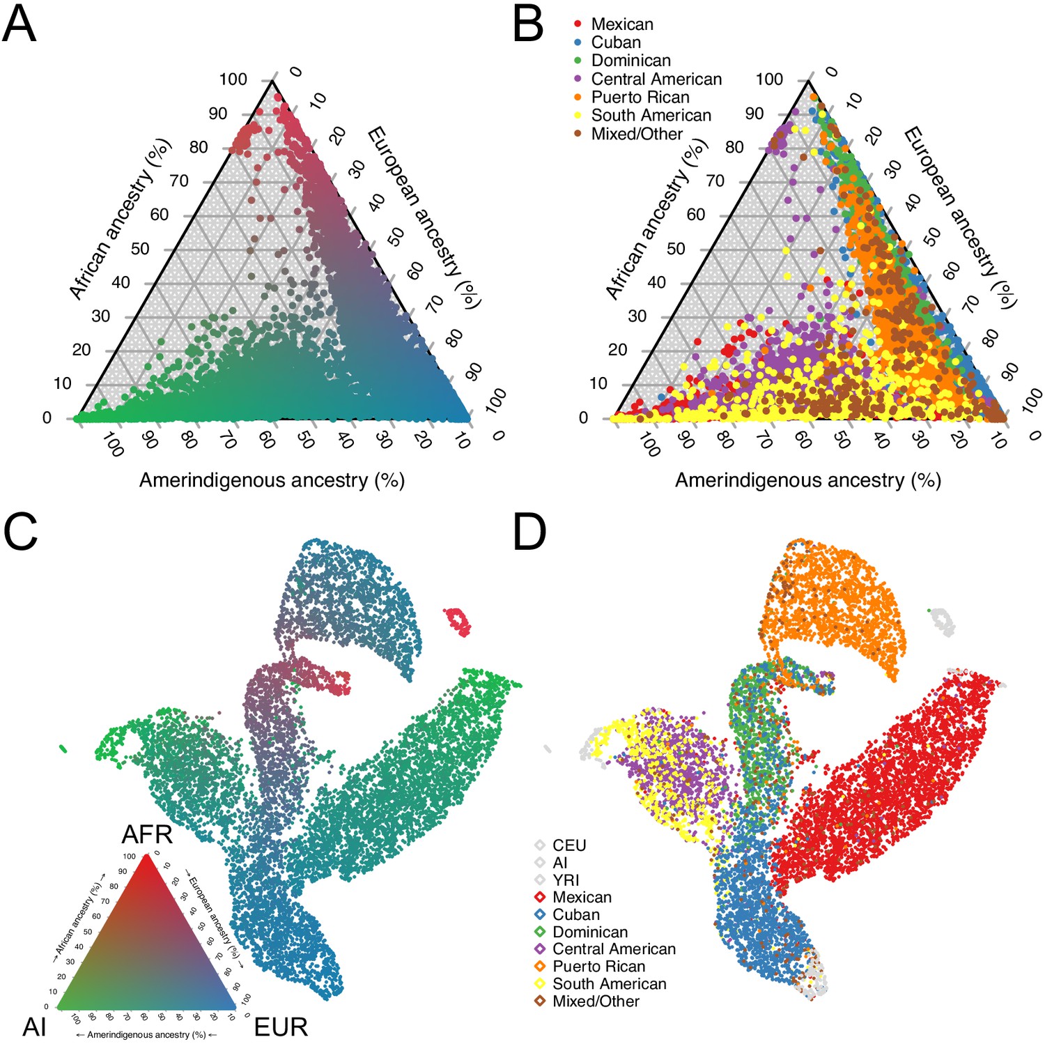
Genomic ancestry and population structure in HCHS/SOL.
(A) Ternary plot of HCHS/SOL (n = 10,268) colored by admixture proportions. (B) Ternary plot of global ancestry proportions colored by population for 10,268 HCHS/SOL individuals (C) Uniform Manifold Approximation and Projection (UMAP) plot depicting the genetic diversity of HCHS/SOL and the reference panel (n = 10,591) using three principal components, colored by admixture proportions Within the legend, AFR, EUR, and AI refer to African, European, and Amerindigenous global ancestries, respectively. (D) UMAP plot of HCHS/SOL and the reference panel (n = 10,591) using three principal components, colored by HCHS/SOL population.
Figure 1—figure supplement 1

Ancestral diversity of HCHS/SOL populations.
(A) Scree plot of principal component analysis of HCHS/SOL and the reference panel (n = 10,591). (B) Uniform Manifold Approximation and Projection (UMAP) plot of HCHS/SOL and the reference panel (n = 10,591) using three principal components, colored by reference population. (C) Uniform Manifold Approximation and Projection (UMAP) plot of HCHS/SOL only (n = 10,591) using three principal components, colored by population. (D) Uniform Manifold Approximation and Projection (UMAP) plot of HCHS/SOL and the larger reference panel (n = 11,567) using three principal components, colored by HCHS/SOL population (E) Uniform Manifold Approximation and Projection (UMAP) plot of HCHS/SOL and the larger reference panel (n = 11,567) using three principal components, colored by African population (F) Uniform Manifold Approximation and Projection (UMAP) plot of HCHS/SOL and the larger reference panel (n = 11,567) using three principal components, colored by Amerindigenous population (G) Uniform Manifold Approximation and Projection (UMAP) plot of HCHS/SOL and the larger reference panel (n = 11,567) using three principal components, colored by European population.
Figure 2 with 5 supplements
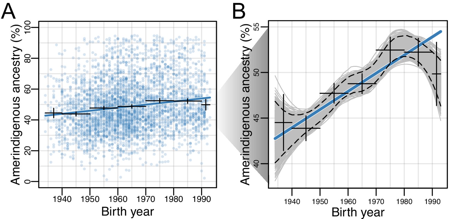
Amerindigenous ancestry has increased over time in Mexican Americans.
(A) Global Amerindigenous ancestry proportions plotted by birth year for Mexican Americans (n = 3,622). Fitted line is multiple regression of Amerindigenous ~ birth year + sampling weight. Bars represent 95% confidence intervals for individuals grouped by decade. (B) Bootstrap resampling (n = 1000 iterations) of Amerindigenous global ancestry for the Mexican American individuals with a fitted LOESS curve for each iteration. Dashed lines represent the 95% quantile range of LOESS curves and the blue line represents the fitted regression line from A.
Figure 2—figure supplement 1
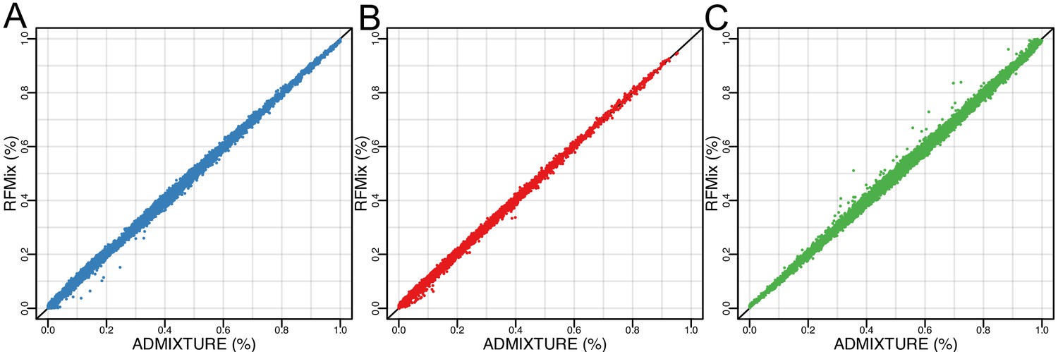
Concordance of ADMIXTURE and RFMix global ancestry estimates.
(A) Amerindigenous ancestry (B) African ancestry and (C) European ancestry.
Figure 2—figure supplement 2
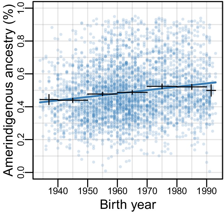
Amerindigenous ancestry has increased over time in Mexican Americans.
RFMix inferred Amerindigenous (AI) global ancestry proportions plotted by birth year for Mexican Americans (n = 3,622). Fitted line is multiple regression of AI global ancestry ~birth year + sampling weight (=0.0022; SE = 0.0002, p<2E-16). Bars represent 95% confidence intervals for individuals grouped by decade.
Figure 2—figure supplement 3
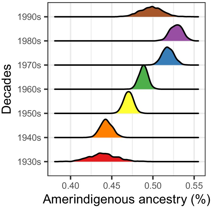
Distributions of Amerindigenous global ancestry means for HCHS/SOL Mexican Americans (n = 3622) generated by 1000 bootstrap resampling iterations within each decade of binned birth years.
Figure 2—figure supplement 4
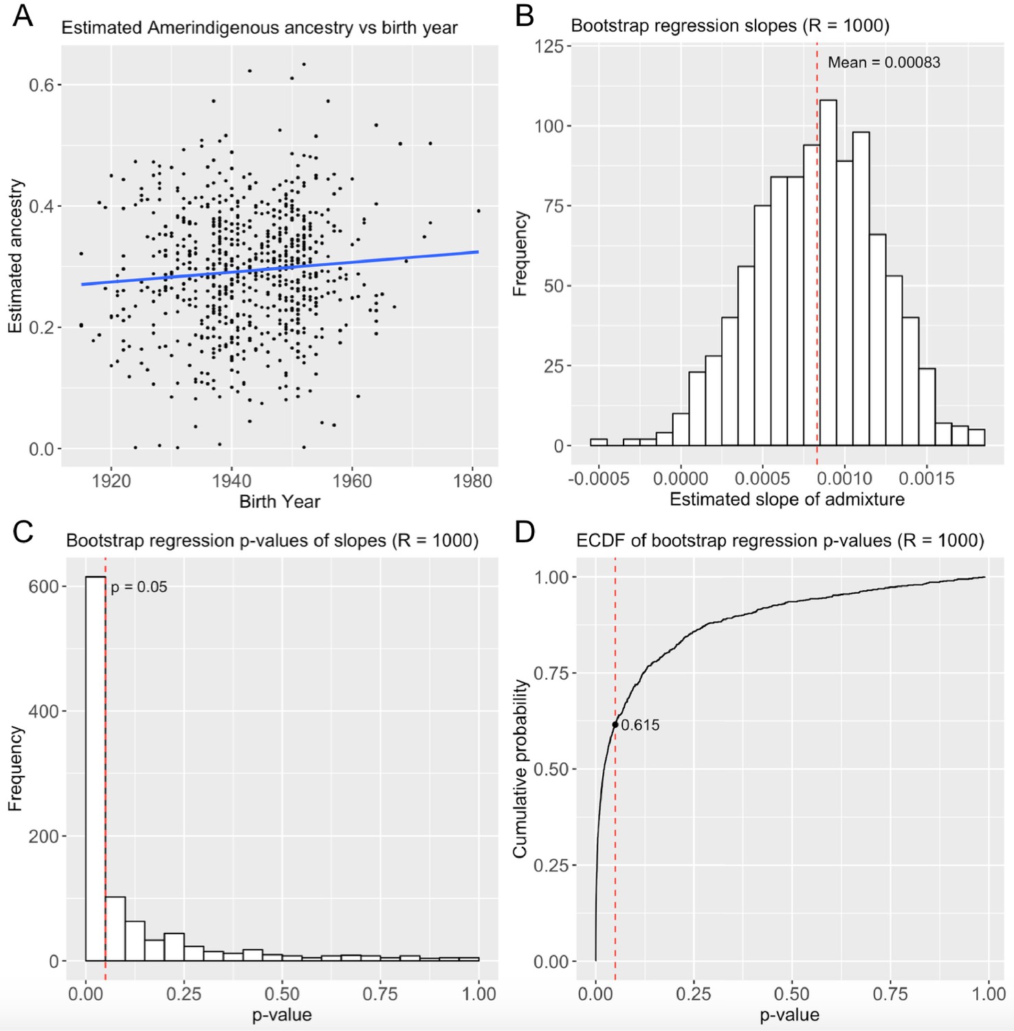
Replication in the Health and Retirement Study for 705 self-identified Mexican Americans.
(A) Ancestry over time (B) Distribution of regression slopes after 1000 bootstrap resampling iterations (C) Distribution of bootstrap regression p-values (D) ECDF of bootstrap regression p-values.
Figure 2—figure supplement 5
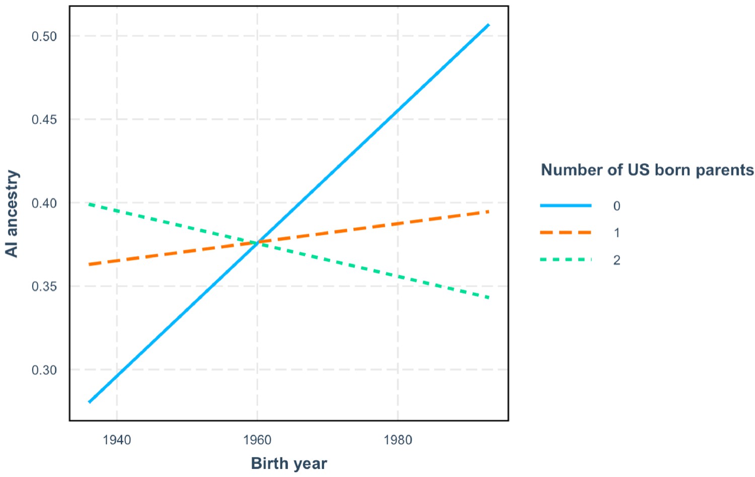
The increase in estimated AI ancestry over time is conditional on the number of US-born parents.
AI ancestry vs birth year with interaction between birth year and number of US-born parents for 634 HCHS/SOL Mexicans.
Figure 3 with 14 supplements
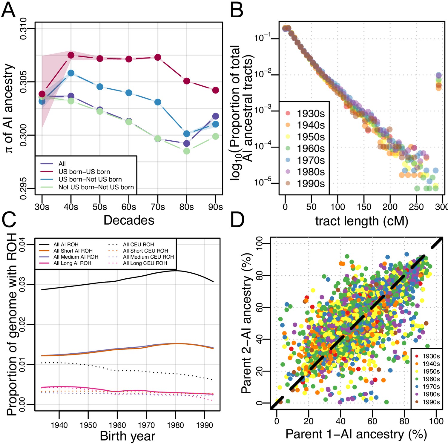
Architecture of genetic diversity in Mexican American Genomes.
(A) Genetic diversity (π) in Amerindigenous ancestry tracts stratified by US-born/not US-born status, and calculated between pairs of individuals born within each decade (with shaded envelopes showing 95% confidence intervals for each group). (B) Proportion of total Amerindigenous (AI) ancestral tracts in the HCHS/SOL Mexican American population by decade. (C) Variation in ROH by birth year. Solid lines show LOESS of the proportion of the genome with AI ancestry that overlap ROH of different lengths, while dotted lines show LOESS of the proportion of the genome with European ancestry that overlap ROH of different lengths. (D) Scatter plot of parents’ inferred global Amerindigenous (AI) ancestries using ANCESTOR.
Figure 3—figure supplement 1
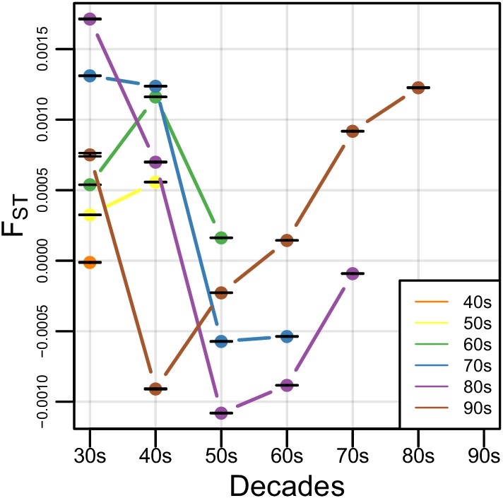
FST within Amerindigenous ancestral tracts.
FST estimates calculated between each decade group. Bars represent the 95% CI.
Figure 3—figure supplement 2
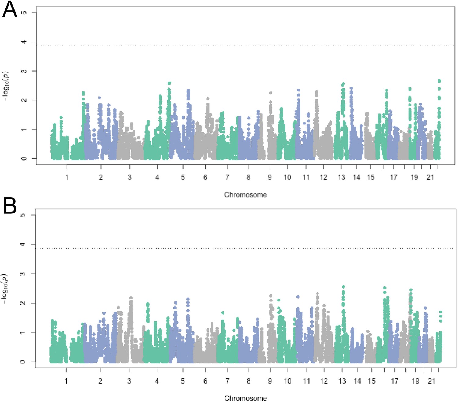
Admixture mapping in HCHS/SOL Mexicans (n = 3622) for Amerindigenous ancestry and (A) birth year and (B) generation.
Ancestry association testing was performed at 211,151 markers using (A) linear regression and (B) logistic regression, both including global Amerindigenous ancestry, sampling weight and center as covariates.
Figure 3—figure supplement 3
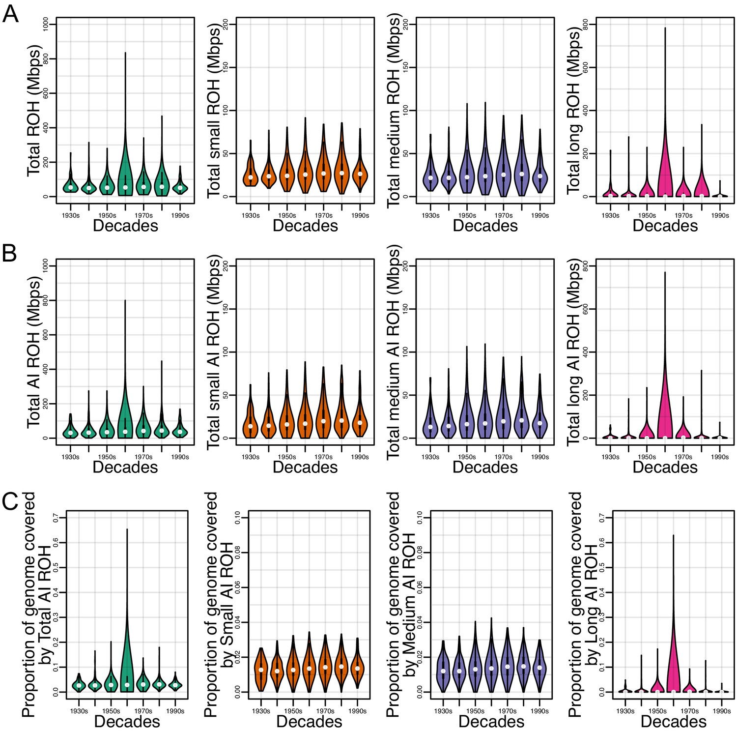
Runs of homozygosity (ROH) in HCHS/SOL Mexican Americans.
(A) ROH (summed per person) across all ancestries separated by ROH class (B) ROH (summed per person) overlapping Amerindigenous (AI) haplotypes separated by ROH class. (C) Proportion of the genome covered by total AI ROH separated by ROH class.
Figure 3—figure supplement 4
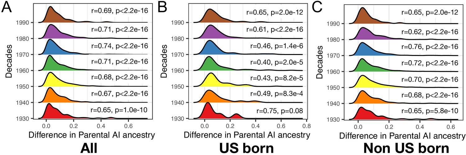
Ancestry-related assortative mating in HCHS/SOL Mexican Americans.
Each distribution represents the difference in inferred parental Amerindigenous (AI) ancestry for each decade for (A) All (B) US-born and (c) Non-US-born. Within each segment is the correlation of parents inferred AI ancestry. Parental ancestry was inferred using ANCESTOR.
Figure 3—figure supplement 5

Standard neutral model simulations result in no change in ancestry proportions over time.
Blue lines show forward simulations while gray lines reproduce the LOESS curves from the observed data shown in Figure 2B.
Figure 3—figure supplement 6

Population growth does not affect the mean ancestry proportions in a population.
(A) The exponential growth rates evaluated. (B–E) The effect of increasing growth rates G={0, 0.1, 0.5, 1} on ancestry proportions.
Figure 3—figure supplement 7
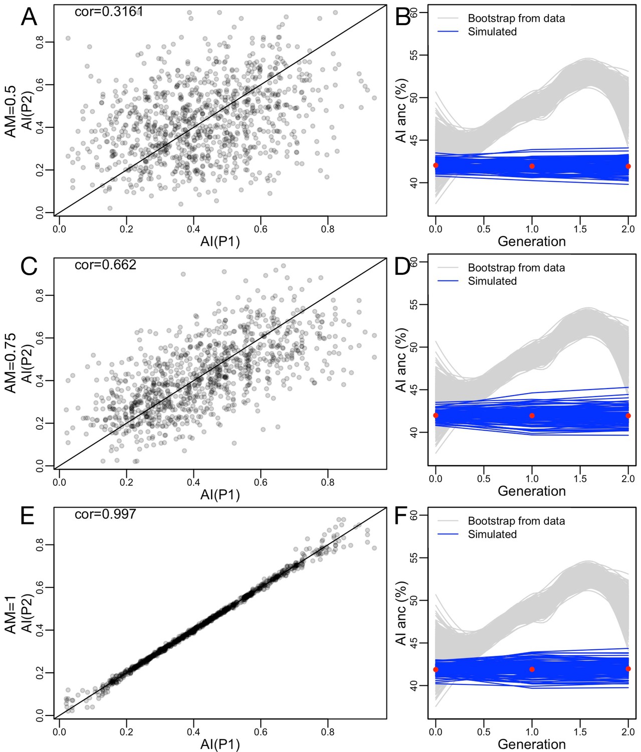
Ancestry-based assortative mating does not change mean ancestry proportions, though variance in ancestry proportions can increase.
(A–B) Low effect of assortative mating, (C–D) moderate effect (with similar correlation to that seen in HCHS Mexican Americans, see main text), and (E–F) extreme assortative mating.
Figure 3—figure supplement 8

Ancestry-based fecundity differences can induce systematic changes in ancestry proportions in a population.
(A) We model the probability of reproducing (‘Prob Reprod’) using a Beta distribution over the ranked ancestry proportions in the population using parameter FAI. (B–E) As ancestry-based fecundity increases, the mean ancestry proportion in the population increases. (F–I) Ancestry-based assortative mating magnifies the effects of ancestry-based fecundity differences (here AM = 0.75, see Figure 3—figure supplement 7).
Figure 3—figure supplement 9
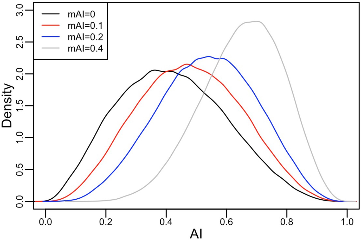
The ancestry proportions in the migrant population are modeled as a Beta distribution, with mean given by a weighted average between the domestic population at one with weight .
When , migrants have the same distribution of ancestry proportions as the domestic population. When , all migrants have 100% Amerindigenous ancestry.
Figure 3—figure supplement 10
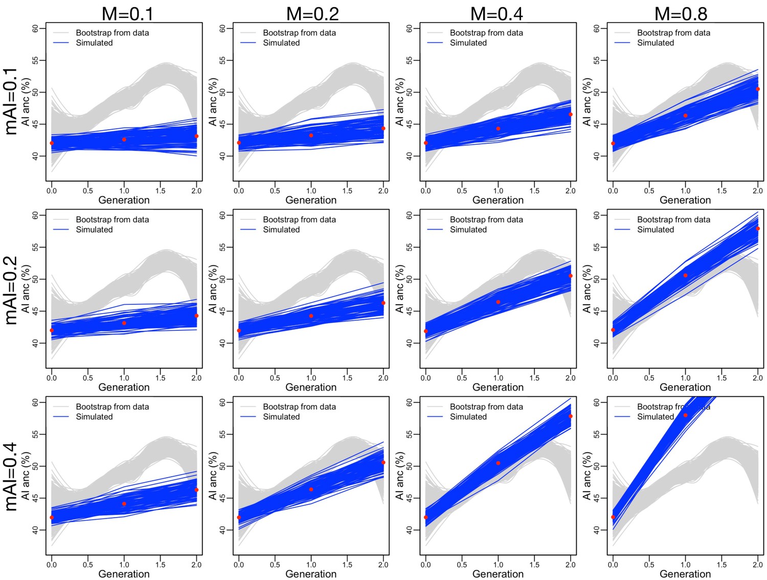
Simulating the effects of migration on changing ancestry proportions.
We show how the ancestry proportions in the domestic population change as we increase (the probability that a new individual is migrant) and (the parameter that governs the ancestry proportions in the migrant population, see Figure 3—figure supplement 9).
Figure 3—figure supplement 11
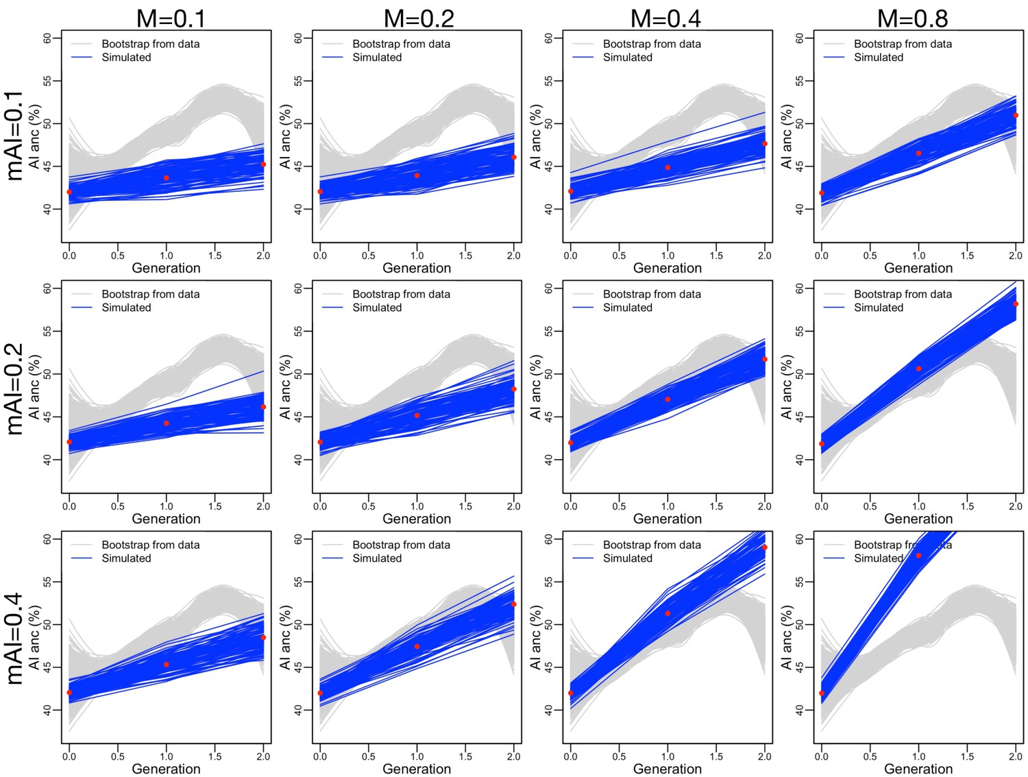
Similar to Figure 3—figure supplement 10, but adding assortative mating (, consistent with our data) and ancestry-based fecundity differences (, see Figure 3—figure supplement 8A).
Figure 3—figure supplement 12
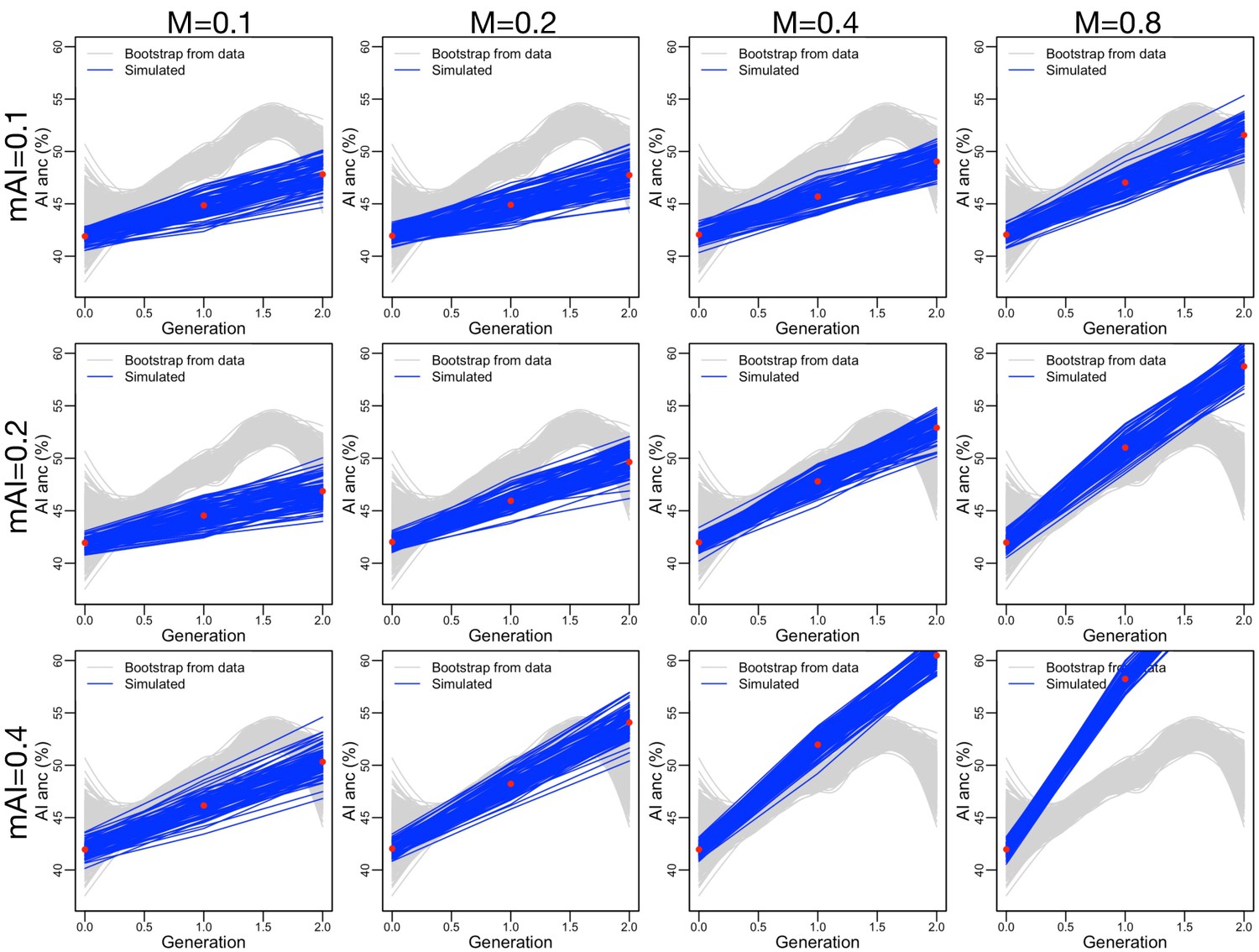
Similar to Figure 3—figure supplement 10, but adding assortative mating (, consistent with our data) and ancestry-based fecundity differences (, see Figure 3—figure supplement 8A).
Figure 3—figure supplement 13
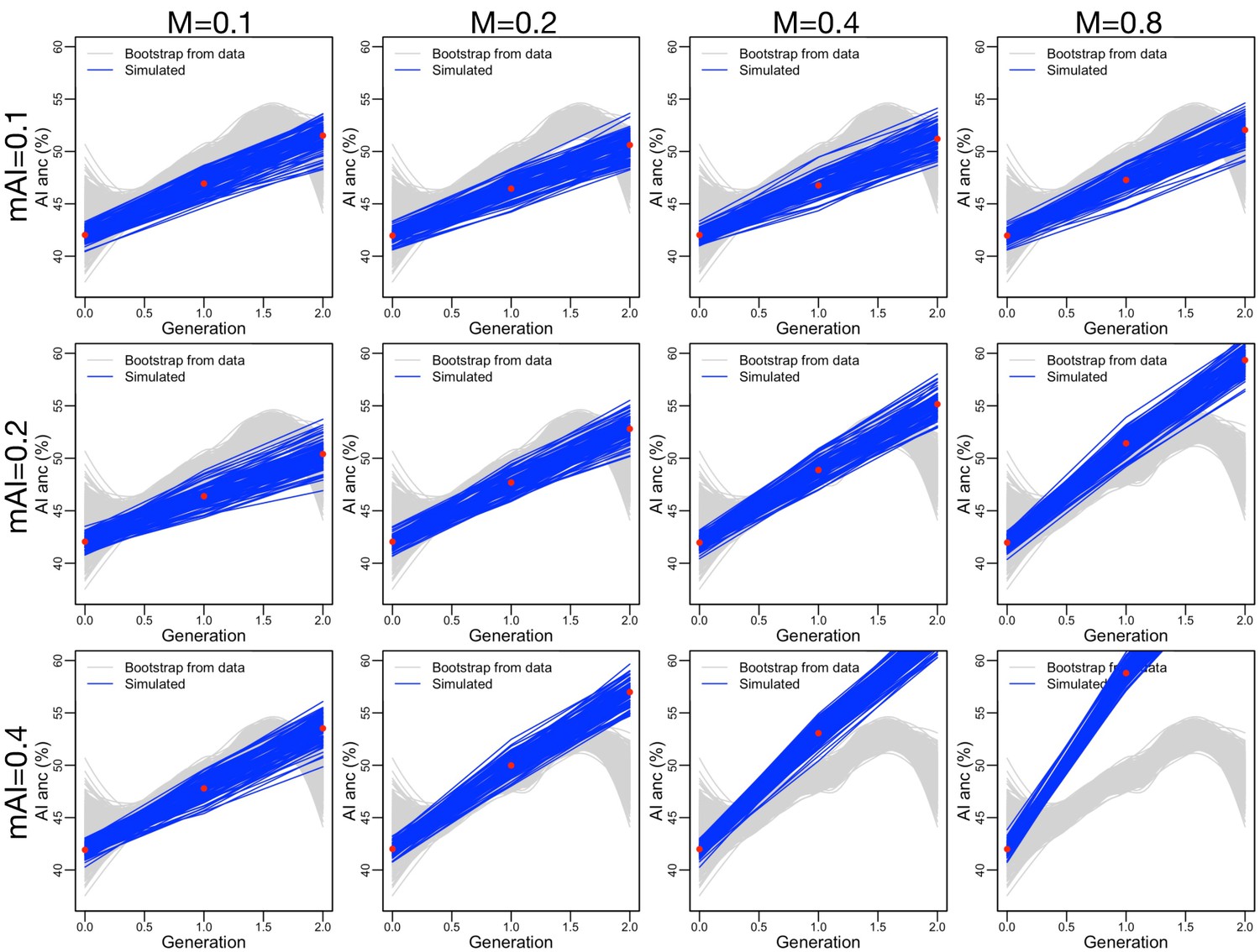
Similar to Figure 3—figure supplement 10, but adding assortative mating (, consistent with our data) and ancestry-based fecundity differences (, see Figure 3—figure supplement 8A).
Figure 3—figure supplement 14

Similar to Figure 3—figure supplement 10, but adding assortative mating (, consistent with our data) and ancestry-based fecundity differences (, see Figure 3—figure supplement 8A).
Figure 4 with 4 supplements

Global Amerindigenous ancestry and biomedical traits in HCHS/SOL Mexican Americans.
(A) The effect size of global AI ancestry on each of 69 quantile normalized traits (see Materials and methods) while controlling for birth year, center, gender, sampling weight, educational attainment, US-born status, and number of US-born parents. (B–C) The relationship between (B) Birth year and height and (C) Height and polygenic height score (PHS). The black line indicates the fitted linear model for all individuals. Each color represents a different quartile of Amerindigenous global ancestry. Polygenic height scores were assessed utilizing UKBB summary statistics for 1,078 SNPs.
Figure 4—figure supplement 1
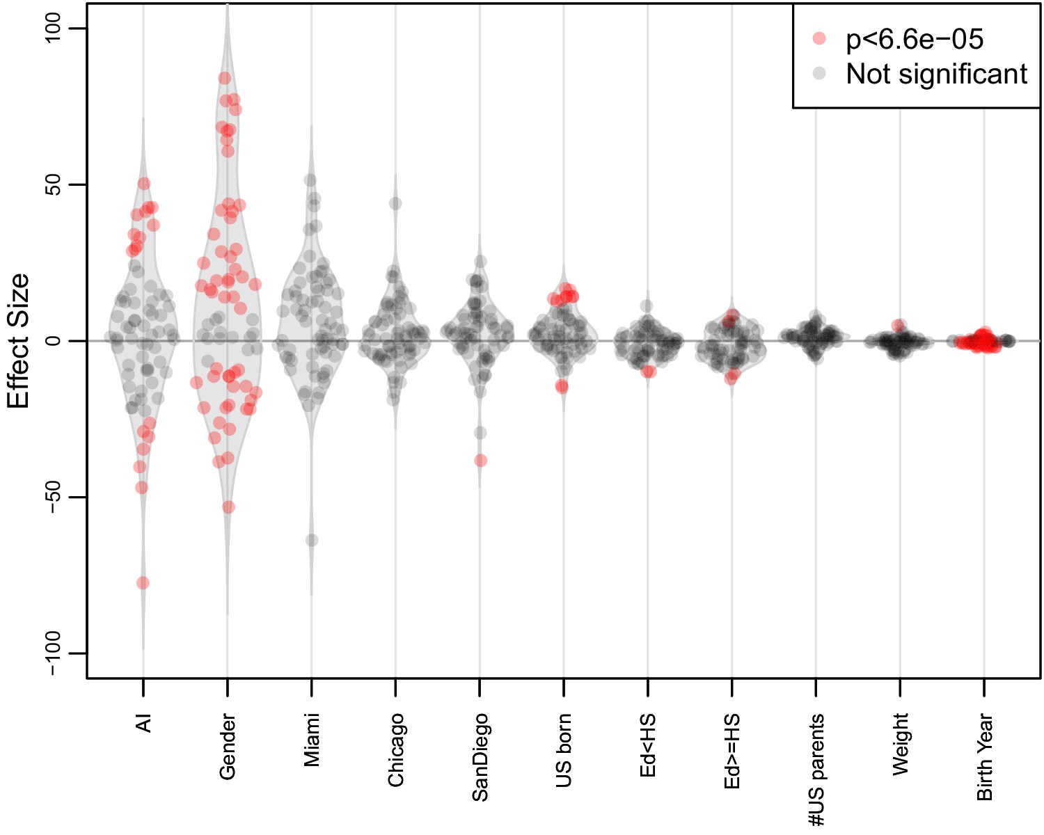
Distribution of variable effects associated with quantile normalized traits.
For 69 biomedical traits we used a multiple linear regression model to analyze the effects of global AI ancestry on each trait while controlling for birth year, center, gender, sampling weight, educational attainment, US-born status, and number of US-born parents. Variables significantly associated with the traits (Bonferroni correction p<6.6E-5) are highlighted in red.
Figure 4—figure supplement 2
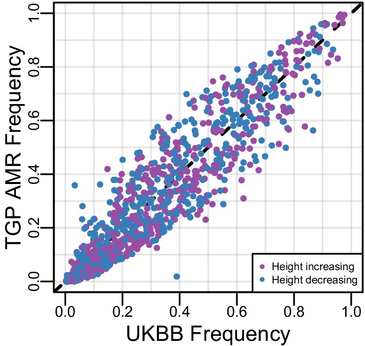
Comparison of allele frequencies used in polygenic height score calculations.
Plotted are the allele frequencies of the non-reference allele in UKBB vs. 1000 Genomes Americas (AMR) population for the 1078 SNPs used to calculate the polygenic height score for the HCHS/SOL Mexican Americans. Colors indicated whether the non-reference allele has a positive or negative effect.
Figure 4—figure supplement 3
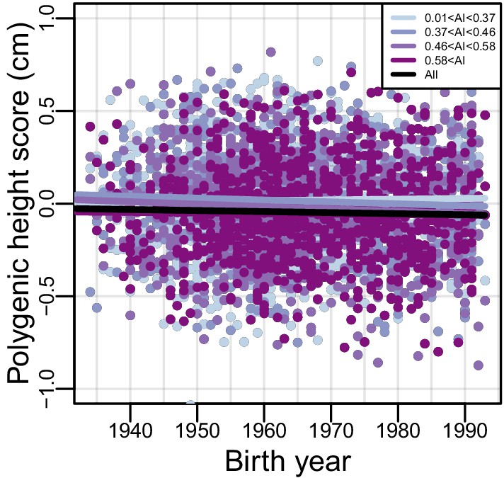
Polygenic height scores over time.
The relationship between birth year and polygenic height score; the black line indicates the fitted linear model for all individuals. Each color represents a different quartile of Amerindigenous global ancestry. Polygenic height scores were assessed utilizing UKBB summary statistics for 1,078 SNPs.
Figure 4—figure supplement 4
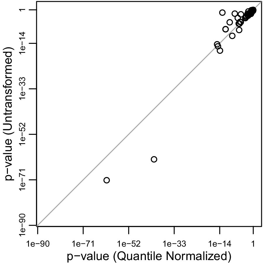
Correlation of 69 p-values for Amerindigenous effect sizes of untransformed vs quantile normalized traits.
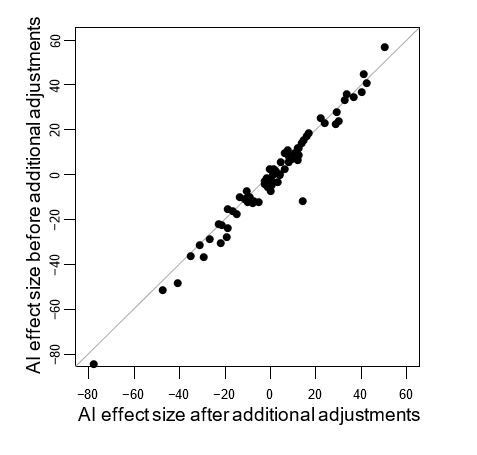
Author response image 1
Tables
Table 1
Relationship of Amerindigenous global ancestry and birth year for Mexican Americans stratified by recruitment region, US-born vs non-US-born status, gender and educational attainment.
For recruitment region, data stratification was limited to Chicago and San Diego as sample size for the Bronx and Miami was limited: 124 and 25 individuals, respectively. Education attainment was categorized as either less than a high school diploma or equivalent degree (<HS), equal to a high school diploma or equivalent degree (=HS), or post-secondary education (>HS). The significance threshold was set at 0.006 using Bonferroni correction for multiple testing (0.05/9).
| Category | N | Mean | Median | R2 | Effect | Std.err | p |
|---|---|---|---|---|---|---|---|
| All | 3622 | 0.489 | 0.468 | 0.027 | 0.0023 | 0.0002 | 3.58E-22 |
| Chicago | 1310 | 0.562 | 0.550 | 0.017 | 0.0016 | 0.0005 | 0.0006 |
| San Diego | 2163 | 0.428 | 0.422 | 0.012 | 0.0012 | 0.0002 | 4.29E-07 |
| US-born | 634 | 0.427 | 0.418 | 0.063 | 0.0027 | 0.0004 | 1.77E-10 |
| Non US-born | 2987 | 0.502 | 0.481 | 0.050 | 0.0032 | 0.0003 | 1.38E-30 |
| Male | 1500 | 0.494 | 0.475 | 0.038 | 0.0028 | 0.0004 | 3.83E-14 |
| Female | 2122 | 0.485 | 0.462 | 0.022 | 0.0019 | 0.0003 | 3.07E-10 |
| <HS | 1518 | 0.520 | 0.500 | 0.045 | 0.0026 | 0.0004 | 1.39E-12 |
| = HS | 960 | 0.501 | 0.479 | 0.022 | 0.0018 | 0.0005 | 0.0003 |
| >HS | 1140 | 0.436 | 0.422 | 0.045 | 0.0027 | 0.0004 | 6.53E-13 |
Additional files
-
Supplementary file 1
Association of global ancestries and birth year for all HCHS/SOL individuals.
For each population, we tested for an association between global ancestry and birth year while accounting for the sampling design. AI, AFR, and EUR refer to Amerindigenous, African, and European ancestry respectively. The significance threshold was set at 0.003 using Bonferroni correction for multiple testing (0.05/18).
- https://cdn.elifesciences.org/articles/56029/elife-56029-supp1-v1.xlsx
-
Supplementary file 2
Frequency table of 3622 HCHS/SOL Mexican Americans stratified by recruitment region, US-born vs non-US-born status, gender and educational attainment.
Recruitment was performed at four regions: Bronx, Chicago, Miami and San Diego. Education attainment was categorized as either less than a high school diploma or equivalent degree (<HS), equal to a high school diploma or equivalent degree (=HS), or post-secondary education (>HS).
- https://cdn.elifesciences.org/articles/56029/elife-56029-supp2-v1.xlsx
-
Supplementary file 3
Association of quantitative traits and Amerindigenous ancestry in HCHS/SOL Mexican Americans.
Each trait as a function of AI ancestry adjusted by birth year, center, gender, sampling weight, educational attainment, US-born status, and number of US-born parents. Results are shown for both the raw data and quantile normalized data.
- https://cdn.elifesciences.org/articles/56029/elife-56029-supp3-v1.xlsx
-
Supplementary file 4
Height over time.
Height (cm) as a function of birth year adjusting by center, gender, sampling weight, educational attainment, US-born status, and number of US-born parents for 3604 Mexican Americans stratified by the quartiles of global Amerindigenous ancestry (AI).
- https://cdn.elifesciences.org/articles/56029/elife-56029-supp4-v1.xlsx
-
Supplementary file 5
Predicted height vs. observed height.
Predicted height (cm) as a function of observed height (cm) adjusting by center, gender, sampling weight, educational attainment, US-born status, and number of US-born parents for 3604 Mexican Americans stratified by Amerindigenous ancestry (AI).
- https://cdn.elifesciences.org/articles/56029/elife-56029-supp5-v1.xlsx
-
Transparent reporting form
- https://cdn.elifesciences.org/articles/56029/elife-56029-transrepform-v1.docx
Download links
A two-part list of links to download the article, or parts of the article, in various formats.
Downloads (link to download the article as PDF)
Open citations (links to open the citations from this article in various online reference manager services)
Cite this article (links to download the citations from this article in formats compatible with various reference manager tools)
Recent shifts in the genomic ancestry of Mexican Americans may alter the genetic architecture of biomedical traits
eLife 9:e56029.
https://doi.org/10.7554/eLife.56029


