A microscopy-based kinetic analysis of yeast vacuolar protein sorting
- Department of Molecular Genetics and Cell Biology, University of Chicago, United States
Figures
Figure 1
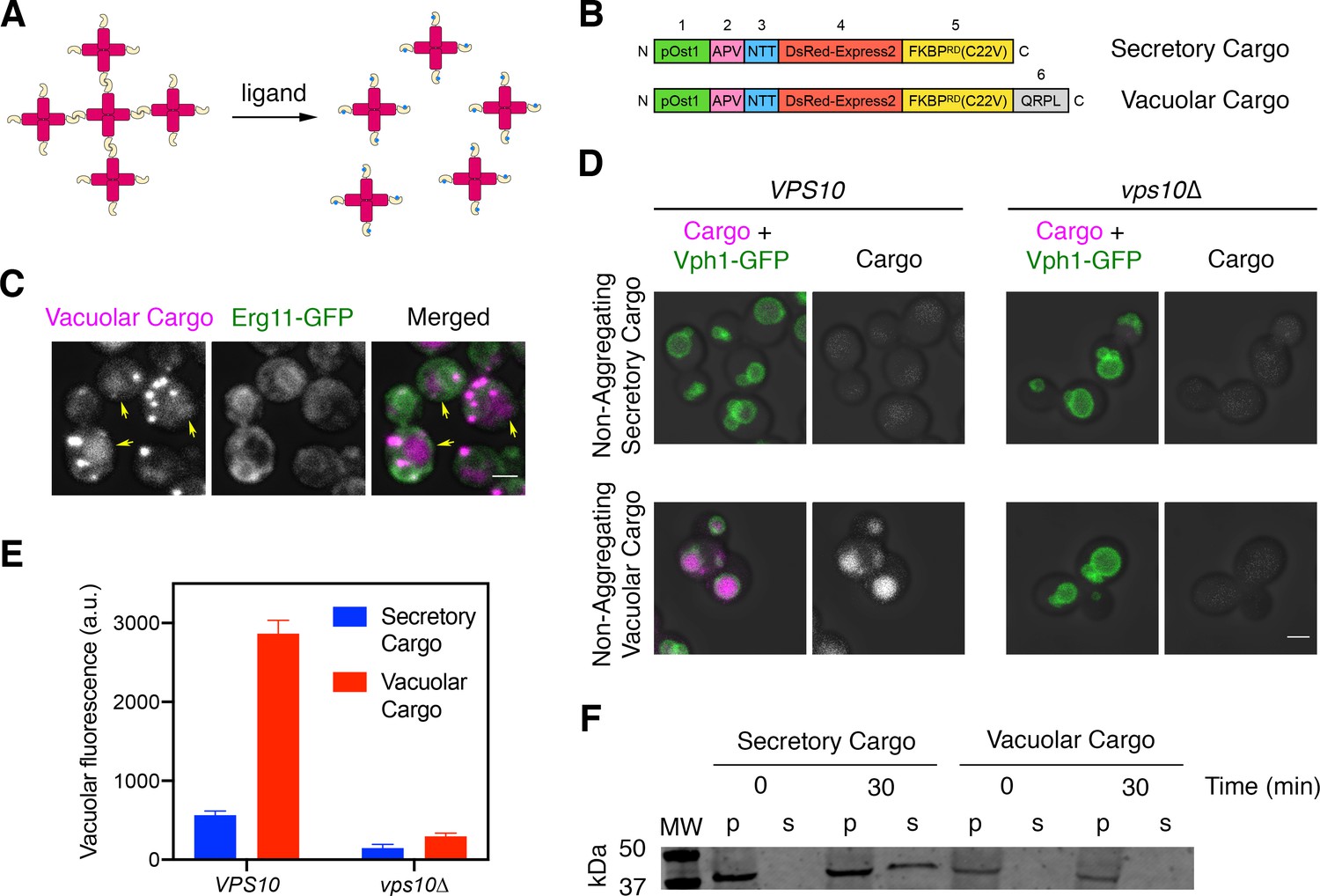
A regulatable vacuolar cargo.
(A) General strategy for the use of reversibly aggregating fluorescent cargoes. DsRed-Express2 tetramers (red) are linked to a dimerizing FKBP variant (gold), so the tetramers associate to form aggregates. Addition of the FKBP ligand SLF (blue) blocks dimerization, thereby dissolving the aggregates into soluble tetramers that can exit the ER. (B) Functional regions of the reversibly aggregating secretory and vacuolar cargoes. The lengths of the regions are not to scale. 1: pOst1 (green) is an ER signal sequence that directs cotranslational translocation. 2: APV (pink) is a tripeptide signal for ER export. 3: NTT (blue) is a tripeptide signal for N-linked glycosylation. 4: DsRed-Express2 (red) is a tetrameric red fluorescent protein. 5: FKBPRD(C22V) (gold) is a reversibly dimerizing variant of FKBP. 6: QRPL (gray) is a tetrapeptide signal for vacuolar targeting. (C) Aggregation in the ER of the vacuolar cargo. The ER membrane marker Erg11-GFP (green) confirms that the aggregates (magenta) are in the ER. Yellow arrows point to leaked cargo molecules that have accumulated in the vacuole. Shown are projected confocal Z-stacks. Scale bar, 2 µm. (D) Vacuolar targeting by the QRPL tetrapeptide. Non-aggregating variants of the secretory and vacuolar cargoes were expressed in VPS10 wild-type or vps10∆ cells to visualize receptor-dependent targeting to the vacuole, which was marked by the vacuolar membrane marker Vph1-GFP. Significant vacuolar accumulation was seen only in the VPS10 background when the QRPL signal was present. Shown are projected confocal Z-stacks. Scale bar, 2 µm. (E) Quantification of the cargo fluorescence signals in (D). The Vph1-GFP signal was used to create a mask for measuring cargo fluorescence in the vacuole. Data are average values from at least 69 cells for each strain. Fluorescence is plotted in arbitrary units (a.u.). Bars represent SEM. (F) Immunoblot to measure cell-associated and secreted levels of the secretory and vacuolar cargoes after SLF addition in rich medium. Cells expressing either the secretory or vacuolar cargo were grown to mid-log phase in YPD, washed with fresh YPD, and treated with SLF. At the 0 and 30 min time points, cell-associated pellet (‘p’) and secreted soluble (‘s’) fractions were separated by centrifugation. Samples were treated with endglycosidase H to trim N-linked glycans, and were analyzed by SDS-PAGE and immunoblotting. Shown is a representative example from four separate experiments. MW, molecular weight markers. The predicted molecular weights for the mature cargoes are ~38–39 kDa. In some samples, the cell-associated vacuolar cargo at the 30 min time point showed evidence of degradation, presumably due to exposure to vacuolar proteases (data not shown).
Figure 2 with 2 supplements
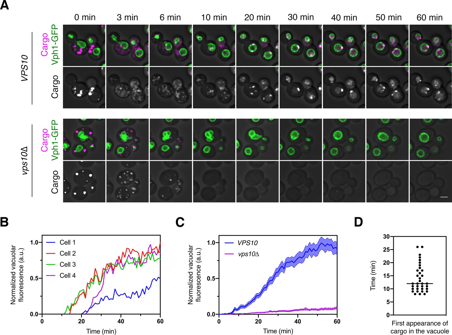
Traffic kinetics of the vacuolar cargo.
(A) Visualizing cargo traffic. The vacuolar cargo expressed in VPS10 wild-type or vps10∆ strains was imaged by 4D confocal microscopy. Prior to the video, fluorescence from leaked cargo molecules was bleached by illuminating the vacuole with a 561 nm laser at maximum intensity for 20–30 s. Then SLF was added, and Z-stacks were captured every minute for 60 min. The top panel shows the cargo (magenta) together with the vacuolar membrane marker Vph1-GFP (green), while the bottom panel shows only the cargo. Fluorescence data are superimposed on brightfield images of the cells. Shown are representative frames from Figure 2—video 1. Scale bar, 2 µm. (B) Quantification of the vacuolar fluorescence from each of the four VPS10 cells in (A). The Vph1-GFP signal was used to create a mask for measuring cargo fluorescence in the vacuole. Fluorescence is plotted in arbitrary units (a.u.). (C) Quantification of the average vacuolar fluorescence in VPS10 and vps10∆ cells after addition of SLF. For each strain, at least 39 cells were analyzed from four movies. Quantification was performed as in (B). The shaded borders represent SEM. (D) Quantification of the first appearance of cargo fluorescence in the vacuole. Data are from the same set of VPS10 cells analyzed for (C). Appearance in the vacuole was scored as the first time point at which the vacuolar cargo fluorescence reached at least 5% of its final value.
Figure 2—figure supplement 1
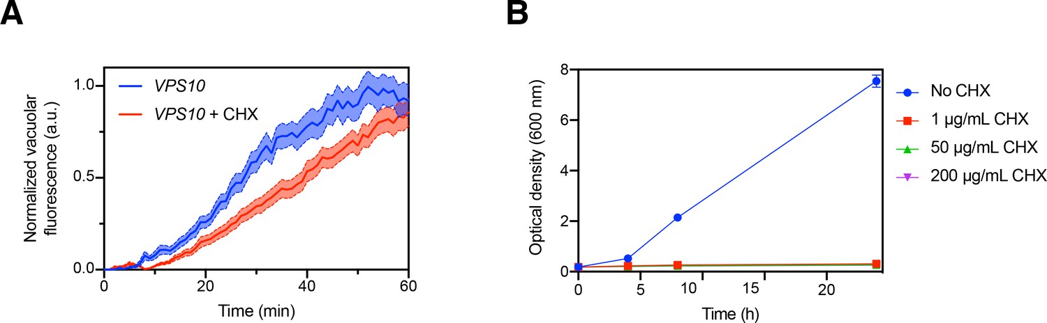
Minor effect of cycloheximide treatment on the kinetics of cargo traffic to the vacuole.
(A) Comparison of traffic kinetics in the absence or presence of cycloheximide (CHX). Data from Figure 2C were re-plotted with the additional analysis of VPS10 cells that had been pretreated with 200 µg/mL cycloheximide starting 15 min prior to addition of SLF. (B) Control experiment to confirm that cycloheximide potently inhibited protein synthesis. A log-phase culture of VPS10 cells in YPD medium was diluted to an OD600 of 0.2, and growth of the culture was measured over 24 hr with or without addition of cycloheximide at the indicated concentrations.
Figure 2—video 1
Visualizing traffic of the vacuolar cargo from the ER to the vacuole.
The cargo expressed in VPS10 wild-type (WT) and vps10∆ strains was imaged by 4D confocal microscopy together with the vacuolar membrane marker Vph1-GFP. Prior to the video, fluorescence from leaked cargo molecules was bleached by illuminating the vacuole with a 561 nm laser at maximum intensity for 20–30 s. Then SLF was added, and Z-stacks were captured every minute for 60 min. In these average projected Z-stacks, fluorescence data are superimposed on brightfield images of the cells. The top panels show the cargo (magenta) together with Vph1-GFP (green), while the bottom panels show only the cargo. Frames from this video are shown in Figure 2A. Scale bar, 2 µm.
Figure 3 with 2 supplements
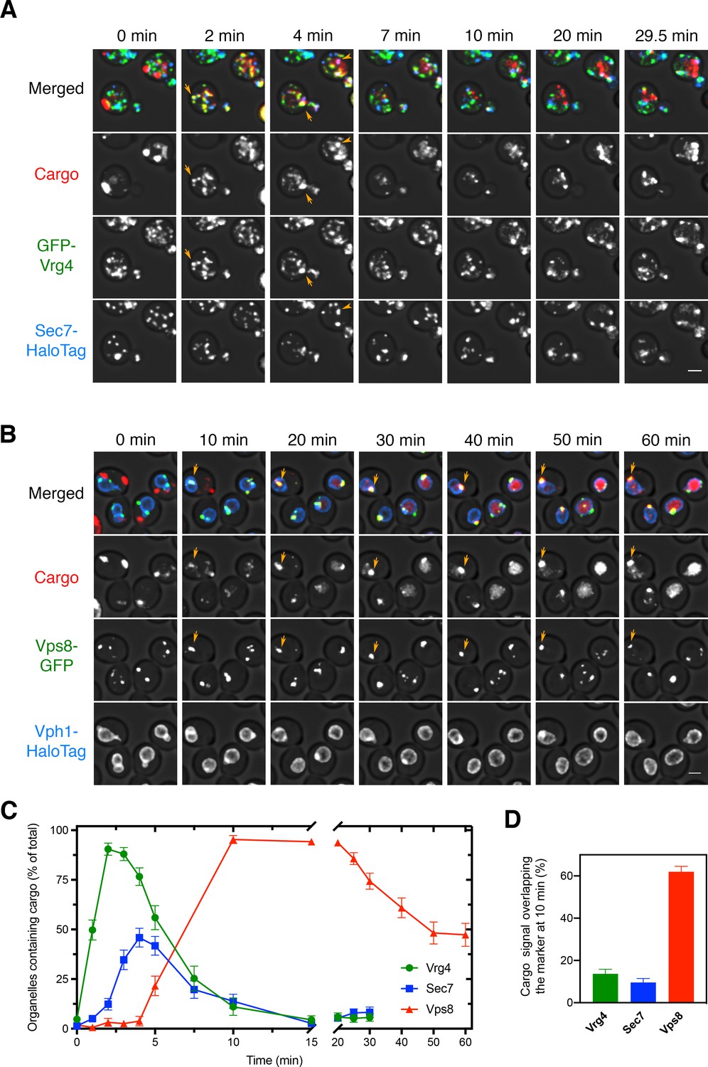
Sequential appearance of the vacuolar cargo in Golgi and PVE compartments.
(A) Appearance of the vacuolar cargo in early Golgi compartments marked with GFP-Vrg4 and in late Golgi compartments marked with Sec7-HaloTag. Cells were grown to mid-log phase, labeled with JF646, and imaged by 4D confocal microscopy. Prior to beginning the video, fluorescence from leaked cargo molecules in the vacuole was bleached by illuminating with maximum intensity 561 nm laser power for 20–30 s. SLF was added directly to the dish between the first and second Z-stacks, and then additional Z-stacks were captured every 30 s for 29.5 min. Images are representative time points from Figure 3—video 1. The top panel shows the merged images, and the other panels show the individual fluorescence channels for cargo, Vrg4, and Sec7. Scale bar, 2 µm. (B) Appearance of the vacuolar cargo in PVE compartments marked with Vps8-GFP and in the vacuole marked with Vph1-HaloTag. The procedure was as in (A), except that Z-stacks were captured every 60 s for 60 min. Images are representative time points from Figure 3—video 2. The top panel shows the merged images, and the other panels show the individual fluorescence channels for cargo, Vps8, and Vph1. Scale bar 2 µm. (C) Quantification of the percentage of compartments containing detectable cargo from (A) and (B). Confocal movies were average projected and manually scored for the presence of cargo in labeled compartments. For each strain, at least 26 cells were analyzed from four movies. The bars represent SEM. (D) Quantification of the percentage of the total cargo fluorescence present in early Golgi, late Golgi, and PVE compartments 10 min after SLF addition. The fluorescence for a compartment marker was used to generate a mask to quantify the corresponding cargo fluorescence. Data were taken from at least 26 cells from four movies. The bars represent SEM.
Figure 3—video 1
Visualizing traffic of the vacuolar cargo together with Golgi markers.
Cells expressing the cargo together with the early Golgi marker GFP-Vrg4 and the late Golgi marker Sec7-HaloTag were grown to mid-log phase, labeled with JF646, and imaged by 4D confocal microscopy. Prior to imaging, fluorescence from leaked cargo molecules in the vacuole was bleached by illuminating with maximum intensity 561 nm laser power for 20–30 s. SLF was added directly to the dish between the first and second Z-stacks, and then additional Z-stacks were captured every 30 s for 29.5 min. In these average projected Z-stacks, fluorescence data are superimposed on brightfield images of the cells. The top panel shows the merged images, and the other panels show the individual fluorescence channels for cargo, Vrg4, and Sec7. Frames from this video are shown in Figure 3A. Scale bar, 2 µm.
Figure 3—video 2
Visualizing traffic of the vacuolar cargo together with PVE and vacuole markers.
Cells expressing the cargo together with the PVE marker Vps8-GFP and the vacuolar membrane marker Vph1-HaloTag were grown to mid-log phase, labeled with JF646, and imaged by 4D confocal microscopy. Prior to imaging, fluorescence from leaked cargo molecules in the vacuole was bleached by illuminating with maximum intensity 561 nm laser power for 20–30 s. SLF was added directly to the dish between the first and second Z-stacks, and then additional Z-stacks were captured every 1 min for 60 min. In these average projected Z-stacks, fluorescence data are superimposed on brightfield images of the cells. The top panel shows the merged images, and the other panels show the individual fluorescence channels for cargo, Vps8, and Vph1. Frames from this video are shown in Figure 3B. Scale bar, 2 µm.
Figure 4 with 3 supplements
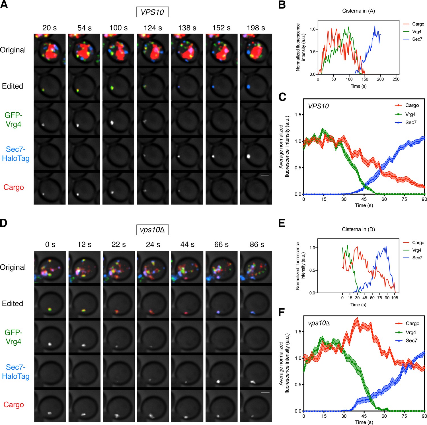
Visualizing the vacuolar cargo during Golgi maturation.
(A) Visualizing the vacuolar cargo in a VPS10 wild-type strain. Cells expressing the vacuolar cargo together with the early Golgi marker GFP-Vrg4 and the late Golgi marker Sec7-HaloTag were grown to mid-log phase, labeled with JF646, and imaged by 4D confocal microscopy. SLF was added 1–3 min before imaging. Shown are average projected Z-stacks at representative time points from Figure 4—video 1. The top row shows the complete projection, the second row shows an edited projection that includes only the cisterna being tracked, and the other rows show the individual fluorescence channels from the edited projection. The large red structure is the vacuole, which contained cargo molecules that had escaped from the ER prior to SLF addition as described in Figure 1. Scale bar, 2 µm. (B) Quantification of the fluorescence intensities of the Golgi markers and the vacuolar cargo during a typical maturation event. Depicted are the normalized fluorescence intensities in arbitrary units (a.u.) of the cisterna tracked in (A). (C) Average cargo signal during the early-to-late Golgi transition. For 21 maturation events from 18 movies of cells expressing moderate levels of the vacuolar cargo, fluorescence was quantified over a 90 s window with Z-stacks collected every 2 s. Normalization was performed by defining the maximum value as the average of the first six fluorescence values for the cargo and Vrg4, or of the last six fluorescence values for Sec7. Traces were aligned at the midpoint of the Vrg4-to-Sec7 transition, and the normalized fluorescence signals were averaged. The shaded borders represent SEM. (D) Visualizing the vacuolar cargo in a vps10∆ strain. The experiment was performed as in (A). Shown are average projected Z-stacks at representative time points from Figure 4—video 2. (E) Quantification of the fluorescence intensities of the Golgi markers and the vacuolar cargo during a typical maturation event in the vps10∆ strain. Depicted are the normalized fluorescence intensities in arbitrary units (a.u.) of the cisterna tracked in (D). (F) Average cargo signal during the early-to-late Golgi transition in a vps10∆ strain. The experiment was performed as in (C). Data were collected for 12 maturation events from 12 movies of cells expressing moderate levels of the vacuolar cargo.
Figure 4—figure supplement 1
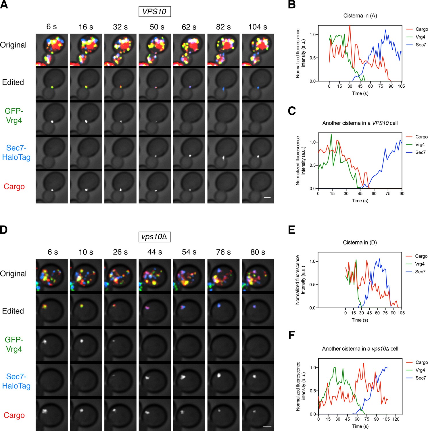
Additional examples of vacuolar cargo traffic during Golgi maturation.
(A) Vacuolar cargo traffic in a VPS10 wild-type strain. The experiment was performed as in Figure 4A. Shown are average projected Z-stacks at representative time points from an additional video. The top row shows the complete projection, the second row shows an edited projection that includes only the cisterna being tracked, and the other rows show the individual fluorescence channels from the edited projection. Scale bar, 2 µm. (B) Quantification of the fluorescence intensities of the Golgi markers and the vacuolar cargo during maturation of the cisterna tracked in (A). The procedure was as in Figure 4B. (C) Quantification of a maturation event from an additional video of a VPS10 cell. (D) – (F) Same as (A) – (C), except that the analysis was performed with a vps10∆ strain.
Figure 4—video 1
Visualizing traffic of the vacuolar cargo during Golgi maturation.
Cells expressing the cargo together with the early Golgi marker GFP-Vrg4 and the late Golgi marker Sec7-HaloTag were grown to mid-log phase, labeled with JF646, and imaged by 4D confocal microscopy. SLF was added 1–3 min before imaging. In these average projected Z-stacks, fluorescence data are superimposed on brightfield images of the cells. The top panel shows the complete projection, the second panel shows an edited projection that includes only the cisterna being tracked, and the other panels show the individual fluorescence channels from the edited projection. Frames from this video are shown in Figure 4A. Scale bar, 2 µm.
Figure 4—video 2
Visualizing traffic of the vacuolar cargo during Golgi maturation in a strain lacking Vps10.
The procedure was as in Figure 4—video 1 except that a vps10∆ strain was used. Frames from this video are shown in Figure 4D. Scale bar, 2 µm.
Figure 5 with 3 supplements

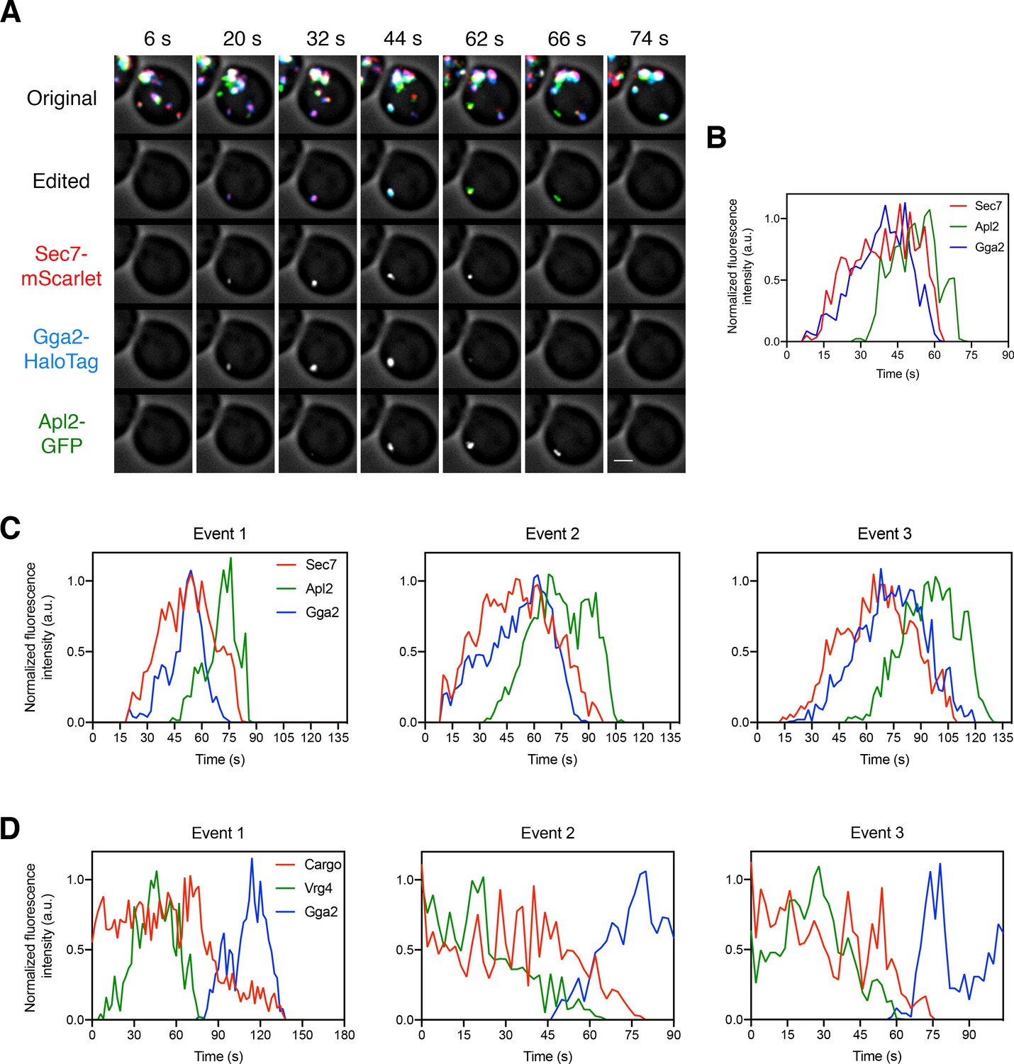
Kinetics of GGA arrival at the Golgi.
(A) Visualizing the dynamics of the GGA and AP-1 adaptors during cisternal maturation. A strain expressing the GGA protein Gga2-HaloTag, the AP-1 subunit Apl2-GFP, and the late Golgi marker Sec7-mScarlet was grown to mid-log phase, labeled with JF646, and imaged by 4D confocal microscopy. Shown are average projected Z-stacks at representative time points from Figure 5—video 1. The top row shows the complete projection, the second row shows an edited projection that includes only the cisterna being tracked, and the other rows show the individual fluorescence channels from the edited projection. Two maturation events are highlighted. Scale bar, 2 µm. (B) Quantification of the fluorescence intensities of the late Golgi marker and the adaptors during typical maturation events. Depicted are the normalized fluorescence intensities in arbitrary units (a.u.) of the two cisternae tracked in (A). (C) Visualizing Vrg4 and Gga2 together with the vacuolar cargo. The experiment was performed as in Figure 4A, except that the Golgi markers were GFP-Vrg4 and Gga2-HaloTag. Shown are average projected Z-stacks at representative time points from Figure 5—video 2. The top row shows the complete projection, the second row shows an edited projection that includes only the cisterna being tracked, and the other rows show the individual fluorescence channels from the edited projection. Scale bar, 2 µm. (D) Quantification of the fluorescence intensities of the Golgi markers together with the vacuolar cargo during a typical maturation event. Depicted are the normalized fluorescence intensities in arbitrary units (a.u.) of the cisterna tracked in (C).
Figure 5—figure supplement 1
Additional examples of adaptor dynamics and of the relationship between GGA arrival and vacuolar cargo departure.
(A) Visualizing the dynamics of the GGA and AP-1 adaptors during cisternal maturation. The experiment was performed as in Figure 5A. Shown are average projected Z-stacks at representative time points from an additional video. The top row shows the complete projection, the second row shows an edited projection that includes only the cisterna being tracked, and the other rows show the individual fluorescence channels from the edited projection. Scale bar, 2 µm. (B) Quantification of the fluorescence intensities of the late Golgi marker and the adaptors during a typical maturation event. Depicted are the normalized fluorescence intensities in arbitrary units (a.u.) of the cisterna tracked in (A). (C) Quantification of the fluorescence intensities of the late Golgi marker and the adaptors during three additional maturation events from three additional movies. The analysis was performed as in (B). (D) Quantification of the fluorescence intensities of the Golgi markers GFP-Vrg4 and Gga2-HaloTag together with the vacuolar cargo during three additional maturation events from three additional movies. The analysis was performed as in Figure 5D.
Figure 5—video 1
Visualizing the dynamics of the GGA and AP-1 clathrin adaptors during Golgi maturation.
Cells expressing the GGA protein Gga2-HaloTag, the AP-1 subunit Apl2-GFP, and the late Golgi marker Sec7-mScarlet were grown to mid-log phase, labeled with JF646, and imaged by 4D confocal microscopy. In these average projected Z-stacks, fluorescence data are superimposed on brightfield images of the cells. The top panel shows the complete projection, the second panel shows an edited projection that includes only the cisterna being tracked, and the other panels show the individual fluorescence channels from the edited projection. Two maturation events are highlighted. Frames from this video are shown in Figure 5A. Scale bar, 2 µm.
Figure 5—video 2
Visualizing the vacuolar cargo together with a GGA adaptor.
Cells expressing the cargo together with the early Golgi marker GFP-Vrg4 and the GGA protein Gga2-HaloTag were grown to mid-log phase, labeled with JF646, and imaged by 4D confocal microscopy. SLF was added 1–3 min before imaging. In these average projected Z-stacks, fluorescence data are superimposed on brightfield images of the cells. The top panel shows the complete projection, the second panel shows an edited projection that includes only the cisterna being tracked, and the other panels show the individual fluorescence channels from the edited projection. Frames from this video are shown in Figure 5C. Scale bar, 2 µm.
Figure 6 with 4 supplements
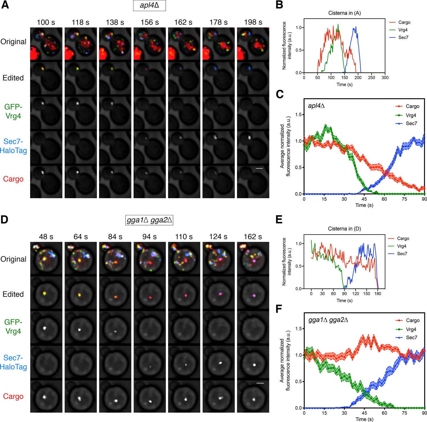
Requirement for the GGAs but not AP-1 during Golgi-to-PVE traffic.
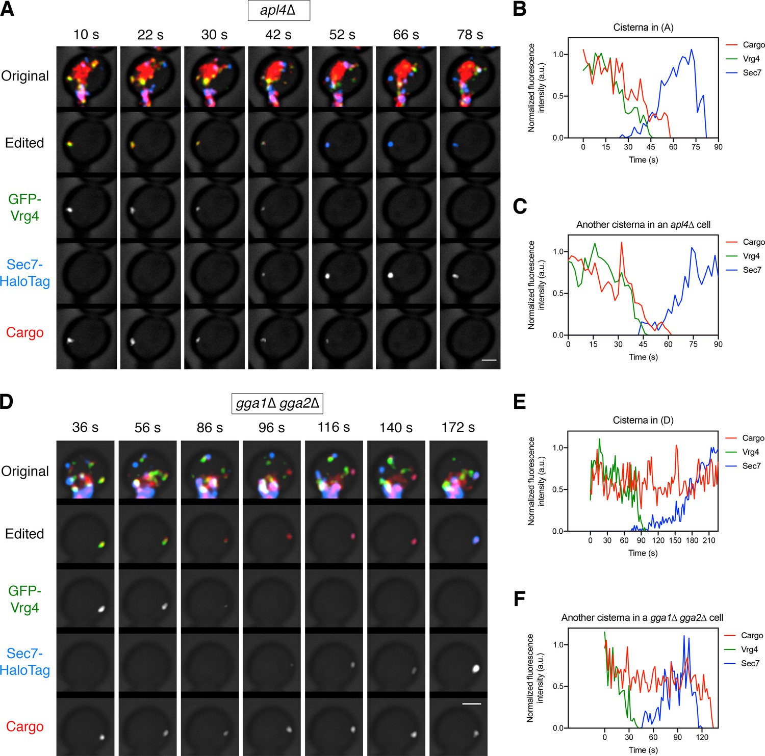
(A) Visualizing vacuolar cargo traffic during Golgi maturation in a strain lacking AP-1. The experiment was performed as in Figure 4A, except that an apl4∆ strain was used. Shown are average projected Z-stacks at representative time points from Figure 6—video 1. The top row shows the complete projection, the second row shows an edited projection that includes only the cisterna being tracked, and the other rows show the individual fluorescence channels from the edited projection. Scale bar, 2 µm. (B) Quantification of the fluorescence intensities of the Golgi markers and the vacuolar cargo during a typical maturation event in the apl4∆ strain. Depicted are the normalized fluorescence intensities in arbitrary units (a.u.) of the cisterna tracked in (A). (C) Average cargo signal during the early-to-late Golgi transition in the apl4∆ strain. The analysis was performed as in Figure 4C, based on 17 maturation events from 13 movies of cells expressing moderate levels of the vacuolar cargo. (D) – (F) Same as (A) – (C) except with a gga1∆ gga2∆ strain lacking GGAs. The analysis in (C) was based on 15 maturation events from 12 movies of cells expressing moderate levels of the vacuolar cargo. Shown in (D) are average projected Z-stacks at representative time points from Figure 6—video 2.
Figure 6—figure supplement 1
Additional examples of cargo dynamics during cisternal maturation in strains lacking AP-1 or GGAs.
(A) Visualizing vacuolar cargo traffic during Golgi maturation in a strain lacking AP-1. The experiment was performed with an apl4∆ strain as in Figure 6A. Shown are average projected Z-stacks at representative time points from an additional video. The top row shows the complete projection, the second row shows an edited projection that includes only the cisterna being tracked, and the other rows show the individual fluorescence channels from the edited projection. Scale bar, 2 µm. (B) Quantification of the fluorescence intensities of the Golgi markers and the vacuolar cargo during maturation of the cisterna tracked in (A). The procedure was as in Figure 6B. (C) Quantification of a maturation event from an additional video of an apl4∆ cell. (D) – (F) Same as (A) – (C) except with a gga1∆ gga2∆ strain lacking GGAs.
Figure 6—figure supplement 2
Secretion of the vacuolar cargo in cells lacking either Vps10 or GGAs.
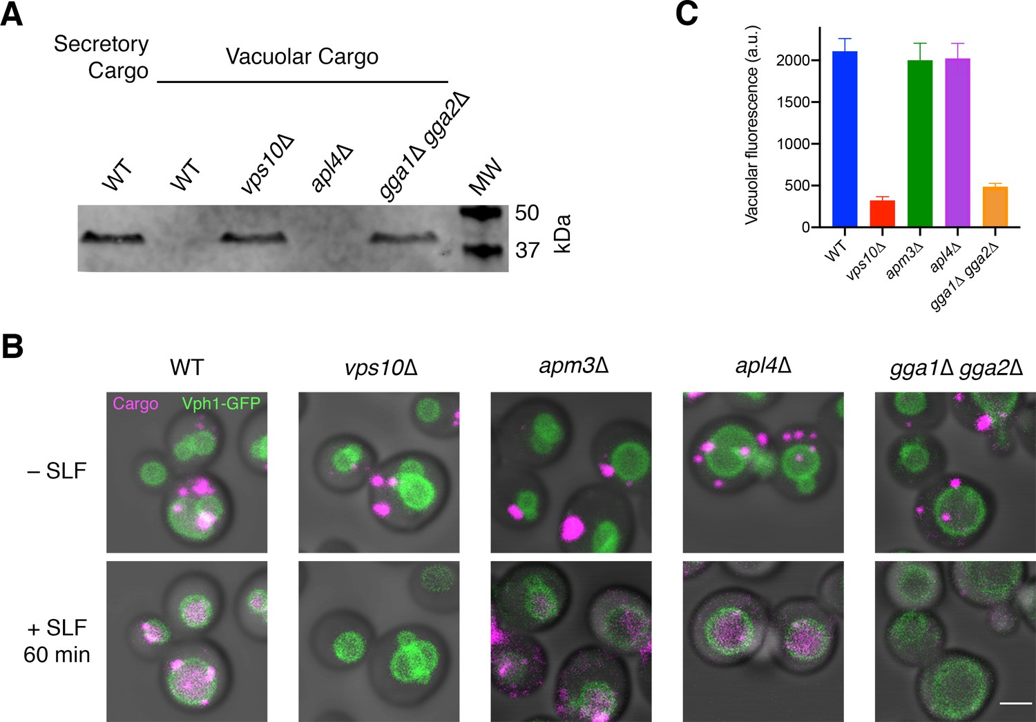
(A) Immunoblot of secreted cargoes after SLF addition in rich medium. Wild-type (WT) cells expressing the secretory cargo and wild-type, vps10∆, apl4∆, and gga1∆ gga2∆ cells expressing the vacuolar cargo were grown to mid-log phase in YPD, washed with fresh YPD, and treated with SLF. After 30 min, the secreted fractions were isolated by centrifugation, treated with endoglycosidase H to trim N-glycans, and analyzed by SDS-PAGE and immunoblotting. Shown is a representative example from four separate experiments. MW, molecular weight markers. The predicted molecular weights for the mature cargoes are ~38–39 kDa. (B) Accumulation of the vacuolar cargo in the vacuole after SLF addition in various genetic backgrounds. The vacuolar cargo was expressed in wild-type, vps10∆, apm3∆, apl4∆, and gga1 gga2∆ cells that also contained the vacuolar membrane marker Vph1-GFP. The experiment was performed as in Figure 2A. (C) Quantification of the amount of cargo reaching the vacuole in (B). The Vph1-GFP signal was used to create a mask for measuring cargo fluorescence in the vacuole. Data are average values from at least 37 cells for each strain. Fluorescence is plotted in arbitrary units (a.u.). Bars represent SEM.
Figure 6—video 1
Visualizing traffic of the vacuolar cargo during Golgi maturation in a strain lacking AP-1.
The procedure was as in Figure 4—video 1 except that an apl4∆ strain was used. Frames from this video are shown in Figure 6A. Scale bar, 2 µm.
Figure 6—video 2
Visualizing traffic of the vacuolar cargo during Golgi maturation in a strain lacking GGAs.
The procedure was as in Figure 4—video 1 except that a gga1∆ gga2∆ strain was used. Frames from this video are shown in Figure 6D. Scale bar, 2 µm.
Figure 7 with 2 supplements
Visualizing transfer of the vacuolar cargo from PVE compartments to the vacuole.
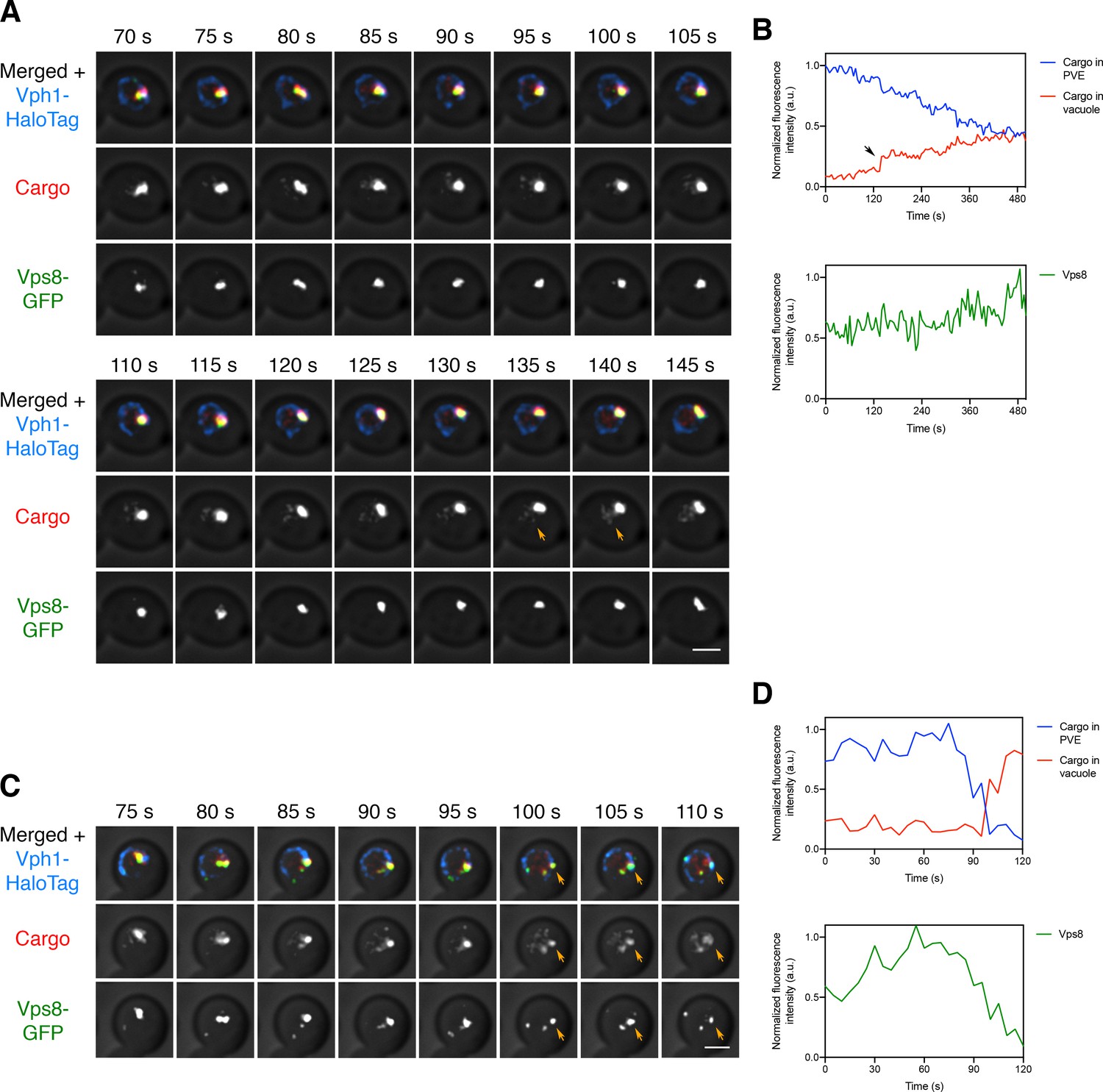
(A) Gradual movement of the vacuolar cargo from a PVE compartment to the vacuole. A strain expressing the vacuolar membrane marker Vph1-HaloTag, the PVE marker Vps8-GFP, and the vacuolar cargo was grown to mid-log phase, attached to a confocal dish, and treated with SLF for 10–15 min to enable the cargo to reach PVE compartments. Prior to imaging, a region that excluded PVE compartments was photobleached by illumination with maximum intensity 561 nm laser light for 40 s. Shown are frames from Figure 7—video 1. The top row shows the complete projection, the middle row shows the cargo fluorescence, and the bottom row shows the Vps8-GFP fluorescence. Orange arrows indicate sudden transfer of a small amount of cargo from the PVE compartment to the vacuole. Scale bar, 2 µm. (B) Quantification from (A) of the time course of cargo fluorescence in the PVE compartment and the vacuole, and of the Vps8 signal. To quantify the cargo signal at each time point, the Vph1 or Vps8 signal was selected in a 3D volume and then the cargo fluorescence within that volume was measured. Normalized data are plotted in arbitrary units (a.u.). The black arrow points to the same cargo transfer event that is marked by the orange arrows in (A). (C) Example of sudden transfer of a large amount of cargo from a PVE compartment to the vacuole. The experiment was performed as in (A). Shown are frames from Figure 7—video 2. Orange arrows indicate an event in which nearly all of the cargo moved from the PVE compartment to the vacuole. (D) Quantification of (C), performed as in (B).
Figure 7—video 1
Visualizing movement of the vacuolar cargo from a PVE compartment to the vacuole.
Cells expressing the cargo together with the vacuolar membrane marker Vph1-HaloTag and the PVE marker Vps8-GFP were grown to mid-log phase, attached to a confocal dish, and treated with SLF for 10–15 min to enable the cargo to reach PVE compartments. Prior to imaging, a region that excluded PVE compartments was photobleached by illumination with maximum intensity 561 nm laser light for 40 s. The top panel shows the complete projection, the middle panel shows the cargo fluorescence, and the bottom panel shows the Vps8-GFP fluorescence. Frames from this video are shown in Figure 7A. Scale bar, 2 µm.
Figure 7—video 2
Visualizing sudden movement of the vacuolar cargo from a PVE compartment to the vacuole.
The procedure was as in Figure 7—video 1. Frames from this video are shown in Figure 7C. Scale bar, 2 µm.
Figure 8 with 5 supplements
Visualizing transfer of Mup1 from PVE compartments to the vacuole.
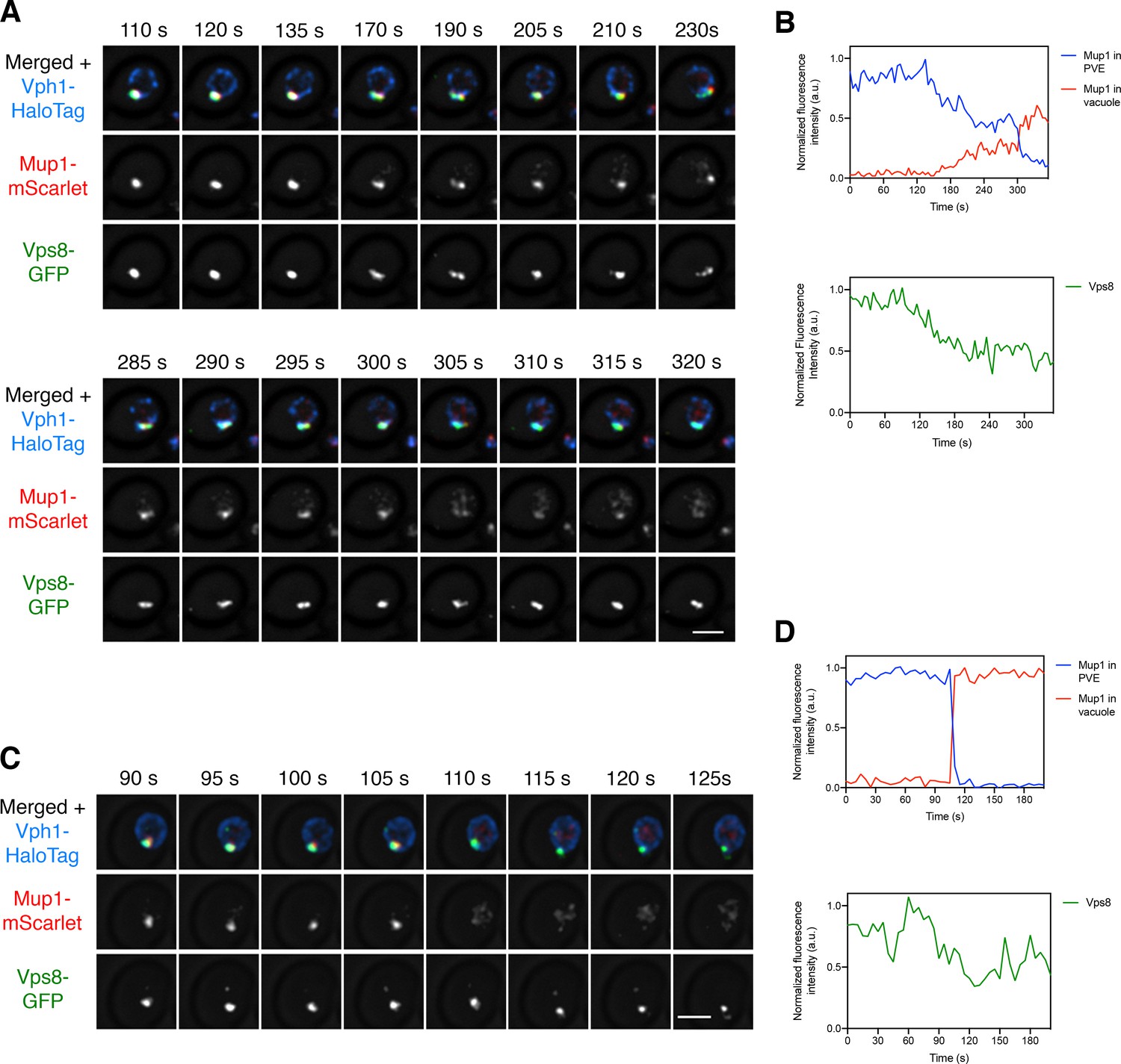
(A) Movement of Mup1 from a PVE compartment to the vacuole. A strain expressing the vacuolar membrane marker Vph1-HaloTag, the PVE marker Vps8-GFP, and Mup1-mScarlet was grown to mid-log phase in NSD lacking methionine, attached to a confocal dish, and exposed to NSD containing methionine for 10–15 min to promote internalization of Mup1 to PVE compartments. Prior to imaging, a region that excluded PVE compartments was photobleached by illumination with maximum intensity 561 nm laser light for 5 s. Shown are frames from Figure 8—video 1, which illustrates a typical example of putative kiss-and-run fusion at about 300 s. The top row shows the complete projection, the middle row shows the Mup1-mScarlet fluorescence, and the bottom row shows the Vps8-GFP fluorescence. Scale bar, 2 µm. (B) Quantification of (A), performed as in Figure 7B. At about 300 s, a significant amount of Mup1 moved from the PVE compartment to the vacuole. (C) Example of an unusually large cargo transfer event. The experiment was performed as in (A), and frames are shown from Figure 8—video 2. Between the 105 s and 110 s time points, virtually all of the Mup1 moved from the PVE compartment to the vacuole. (D) Quantification of (C), performed as in Figure 7B.
Figure 8—figure supplement 1
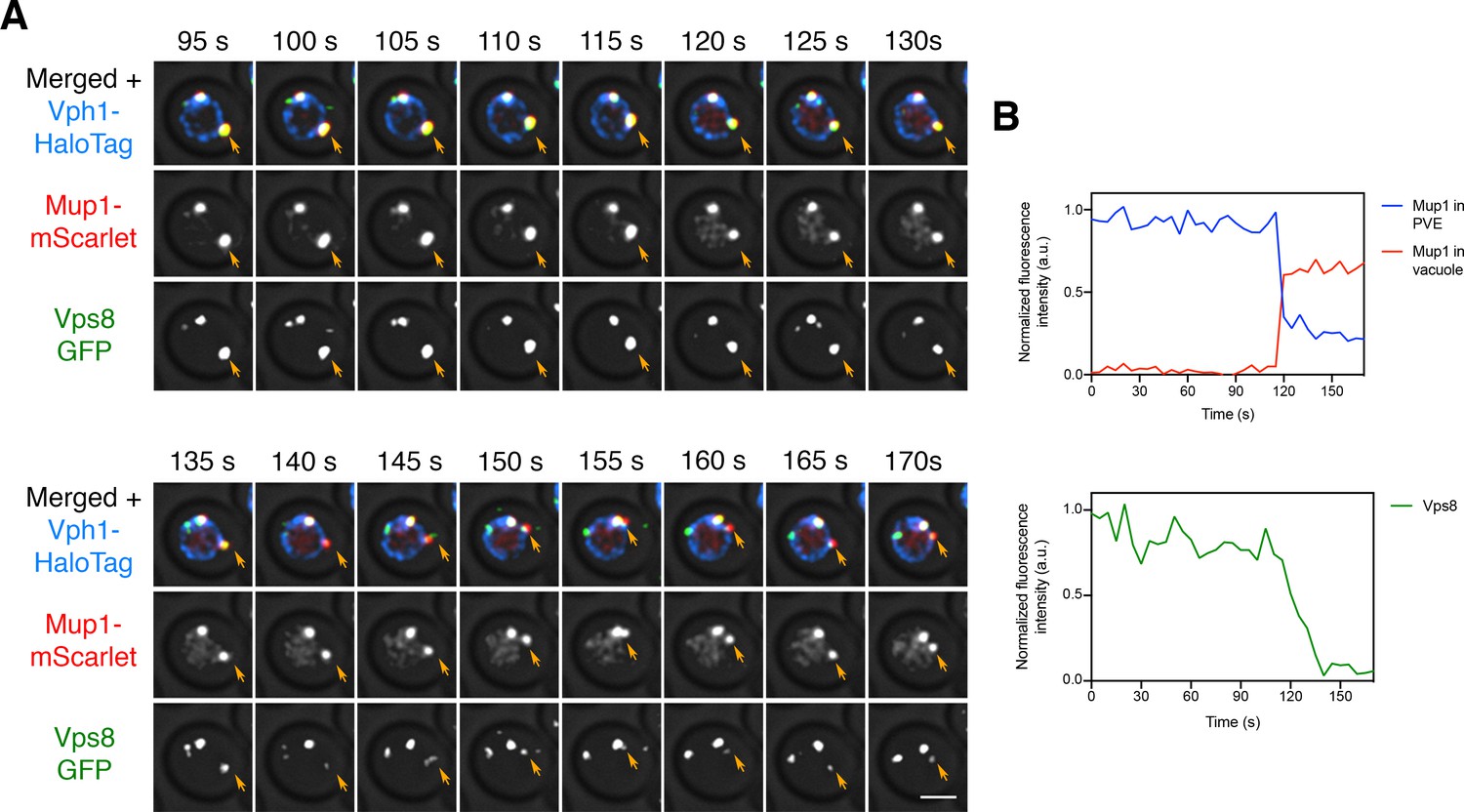
Reduction in Vps8 labeling of a PVE compartment after a large cargo transfer event.
(A) Sudden movement of Mup1 from a PVE compartment to the vacuole. The experiment was performed as in Figure 8A, and frames are shown from Figure 8—video 3. Orange arrows indicate the PVE compartment that was tracked. (B) Quantification of (A), performed as in Figure 7B. Between the 115 s and 120 s time points, a large fraction of the Mup1 moved from the PVE compartment to the vacuole, and the Vps8-GFP fluorescence began a steep decline.
Figure 8—figure supplement 2
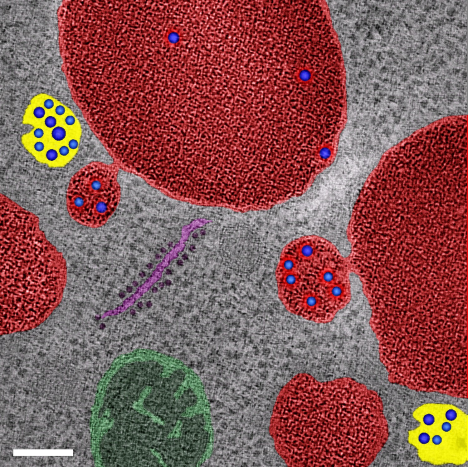
Evidence from previously published electron tomography data (McNatt et al., 2007) for partial fusion of PVE compartments with the vacuole.
This image shows electron tomography of vacuoles and associated PVE compartments in S. cerevisiae. Non-fused PVE compartments are yellow, vacuoles are red, and PVE compartments with tubular connections to the vacuole are also red to reflect the luminal continuity. Intraluminal vesicles are blue. Also shown are a mitochondrion (green) and a piece of ribosome-studded ER (purple). Scale bar, 100 nm.
© 2007 West and Odorizzi. This cover image for the February 2007 issue of Molecular Biology of the Cell (Volume 18, Number 2) was kindly provided by Matt West and Greg Odorizzi, and is reprinted here with permission, under the terms of a CC-BY-NC-SA 3.0 license. This image is not covered by the CC-BY 4.0 license, and further reproduction must adhere to the terms of the CC-BY-NC-SA 3.0 license (https://creativecommons.org/licenses/by-nc-sa/3.0/).
Figure 8—video 1
Visualizing movement of Mup1 from a PVE compartment to the vacuole.
Cells expressing the vacuolar membrane marker Vph1-HaloTag, the PVE marker Vps8-GFP, and Mup1-mScarlet were grown to mid-log phase in NSD lacking methionine, attached to a confocal dish, and exposed to NSD containing methionine for 10–15 min to promote internalization of Mup1 to PVE compartments. Prior to imaging, a region that excluded PVE compartments was photobleached by illumination with maximum intensity 561 nm laser light for 5 s. The top panel shows the complete projection, the middle panel shows the Mup1-mScarlet fluorescence, and the bottom panel shows the Vps8-GFP fluorescence. Frames from this video are shown in Figure 8A. Scale bar, 2 µm.
Figure 8—video 2
Visualizing sudden movement of Mup1 from a PVE compartment to the vacuole.
The procedure was as in Figure 8—video 1. Frames from this video are shown in Figure 8C. Scale bar, 2 µm.
Figure 8—video 3
Reduction in the apparent size of a PVE compartment after a large cargo transfer event.
The procedure was as in Figure 8—video 1. Frames from this video are shown in Figure 8—figure supplement 1A. Scale bar, 2 µm.
Figure 9

Model for sorting of biosynthetic cargoes in the late Golgi.
(A) Sequential formation of GGA vesicles and AP-1 vesicles in yeast cells. The thick arrows represent progressive maturation of a Golgi cisterna over time. During the early-to-late Golgi transition of cisternal maturation, GGA adaptors arrive, and GGA vesicles that carry vacuolar cargoes (white squares) begin to form. Subsequently, the AP-1 adaptor arrives, and AP-1 vesicles that recycle resident Golgi proteins (not shown) as well as some secretory cargoes (black dots) begin to form. GGAs depart before AP-1 departs, but the formation phases for GGA vesicles and AP-1 vesicles overlap. (B) Comparison of Golgi structures in yeast and mammalian cells. In S. cerevisiae, the late Golgi or TGN stage accounts for about half of the maturation process, so the sequential arrival times and activities of GGAs and AP-1 are easy to detect. In mammalian cells, Golgi cisternae are stacked, with the youngest early Golgi cisterna at the opposite side of a stack from the oldest late Golgi/TGN cisterna. Only the trans-most cisterna of a mammalian Golgi stack functions as late Golgi/TGN, but during the lifetime of this cisterna, GGAs and AP-1 may arrive and act sequentially as in yeast.
Tables
Key resources table
| Reagent type (species) or resource | Designation | Source or reference | Identifiers | Additional information |
|---|---|---|---|---|
| Chemical compound, drug | Hygromycin | Thermo Fisher | Cat. #: 10687010 | |
| Chemical compound, drug | G418 | Teknova | Cat. #: G5001 | |
| Chemical compound, drug | Nourseothricin | Neta Scientific | Cat. #: RPI-N51200-1.0 | |
| Chemical compound, drug | JF646 HaloTag Ligand | Dr. Luke Lavis (Janelia Research Campus) Grimm et al., 2015 | ||
| Chemical compound, drug | SLF | Cayman Chemical | Cat. #: 10007974–5 | |
| Chemical compound, drug | Cycloheximide | Neta Scientific | Cat. #: RPI-C81040-1.0 | |
| Chemical compound, drug | Concanavalin A | Sigma-Aldrich | Cat. #: C2010-250MG | |
| Antibody | anti-FKBP12 (rabbit polyclonal) | Abcam | Cat. #: ab2918 | WB (1:1000) |
| Antibody | Alexa Fluor 647 anti-rabbit (goat polyclonal) | Thermo Fisher | Cat. #: A21245 | WB (1:1000) |
| Software, algorithm | Graphpad Prism | Insightful Science (https://www.graphpad.com) | RRID:SCR_002798 | |
| Software, algorithm | SnapGene | Insightful Science (https://www.snapgene.com) | RRID:SCR_015052 | |
| Software, algorithm | ImageJ | ImageJ (https://imagej.nih.gov/ij/) | RRID:SCR_003070 |
Table 1
Primers used in this study.
| Purpose | Amplifies | Primers |
|---|---|---|
| PDR1 deletion | kanMX resistance cassette | 5’-CAGCCAAGAATATACAGAAAAGAATCCAAGAAACTGGAAGCGTACGCTGCAGGTCGAC-3’ 5’-GGAAGTTTTTGAGAACTTTTATCTATACAAACGTATACGTATCGATGAATTCGAGCTCG-3’ |
| PDR3 deletion | Nourseothricin resistance cassette | 5’-ATCAGCAGTTTTATTAATTTTTTCTTATTGCGTGACCGCACGTACGCTGCAGGTCGAC-3’ 5’-TACTATGGTTATGCTCTGCTTCCCTATTTTCTTTGCGTTTATCGATGAATTCGAGCTCG-3’ |
| GGA1 deletion | Hygromycin resistance cassette | 5’-AGTCACTACTTCAAGTATAACCCAGACAAGAGTCTTTTAAATAGCTTGCCTTGTCCCCGC-3’ 5’-ATGGCATCTACTTTTTTTTCAACTTCTCTACCGAATTTGACGTTTTCGACACTGGATGGC-3’ |
| VPS10 deletion | VPS10 5’ upstream | 5’-CCCAAACTAAAAAGTATCCGCCTGT-3’ 5’-GACAAGGCAAGCTAACGTGTGATGACTACTGGACACT-3’ |
| VPS10 3’ downstream | 5’-GCCATCCAGTGTCGAAGAGATTACTTTACATAGAGTAGATAATTCCATATACTTTTCATA −3’ 5’-AATGAAGTACTATAAATATTAAAGTACGTTAGTAGTTTATTTCTCTTCGG-3’ | |
| Hygromycin resistance cassette | 5’-TCATCACACGTTAGCTTGCCTTGTCCCCGC-3’ 5’-TGTAAAGTAATCTCTTCGACACTGGATGGCGG-3’ | |
| APM3 deletion | APM3 5’ upstream | 5’-AGGGGTAGAAGTCGCTGATTGAT-3’ 5’-GGGCCTCCATGTCCTATTTTGGTTGGGTTGGTAAGGTTTACAG-3’ |
| APM3 3’ downstream | 5’-GCTGGTCGCTATACTGTTATATGTGTACTTGAAATTCCATGCGAAACTAAA-3’ 5’-TGCGGAAGTCTTCCCTAAGACG-3’ | |
| Hygromycin resistance cassette | 5’-CAACCAAAATAGGACATGGAGGCCCAGAATACCC-3’ 5’-TCAAGTACACATATAACAGTATAGCGACCAGCATTCACA-3’ | |
| APL4 deletion | APL4 5’ upstream | 5’-ATGTATATAATTCCGGAAGTGTGGTCCT-3’ 5’-GACAAGGCAAGCTTATGGTGTTCAGGTCTTTCTCGTTGCT-3’ |
| APL4 3’ downstream | 5’-CCATCCAGTGTCGAAAAATGCCTTTAAAATTACAGAACATAACATGATTAATGAC-3’ 5’-GAATTCTGGTCCAAGGCAATTCTATATTTGAT-3’ | |
| Hygromycin resistance cassette | 5’-CCTGAACACCATAAGCTTGCCTTGTCCCCG-3’ 5’-TTTTAAAGGCATTTTTCGACACTGGATGGCGG-3’ | |
| GGA2 deletion | GGA2 5’ upstream | 5’-GATTTCTACAGTCTTTCTGATGGGTTCTTGG-3’ 5’-ACGATATTCTTAGACATGATGCAGTATCACGATTAGCAAT-3’ |
| GGA2 3’ downstream | 5’-AATCTTGGCTTAATCCTCTGGCGTTTCTTATCAATCCTTTCT-3’ 5’-TCTTCCTTTGAAGAAAATTCGTCCTCATCT-3’ | |
| K. lactis LEU2 | 5’-AATCGTGATACTGCATCATGTCTAAGAATATCGTTGTCCTACCGG-3’ 5’-GAAACGCCAGAGGATTAAGCCAAGATTTCCTTGACAGCC-3’ | |
| Integration at TRP1 | TRP1 locus | 5’-GTGTACTTTGCAGTTATGACG-3’ 5’-AGTCAACCCCCTGCGATGTATATTTTCCTG-3’ |
Additional files
-
Supplementary file 1
Plasmid files.
- https://cdn.elifesciences.org/articles/56844/elife-56844-supp1-v2.zip
-
Transparent reporting form
- https://cdn.elifesciences.org/articles/56844/elife-56844-transrepform-v2.docx
Download links
A two-part list of links to download the article, or parts of the article, in various formats.
Downloads (link to download the article as PDF)
Open citations (links to open the citations from this article in various online reference manager services)
Cite this article (links to download the citations from this article in formats compatible with various reference manager tools)
A microscopy-based kinetic analysis of yeast vacuolar protein sorting
eLife 9:e56844.
https://doi.org/10.7554/eLife.56844


