A theory of joint attractor dynamics in the hippocampus and the entorhinal cortex accounts for artificial remapping and grid cell field-to-field variability
- Edmond and Lily Safra Center for Brain Sciences, The Hebrew University of Jerusalem, Israel
- Racah Institute of Physics, The Hebrew University of Jerusalem, Israel
Figures
Figure 1
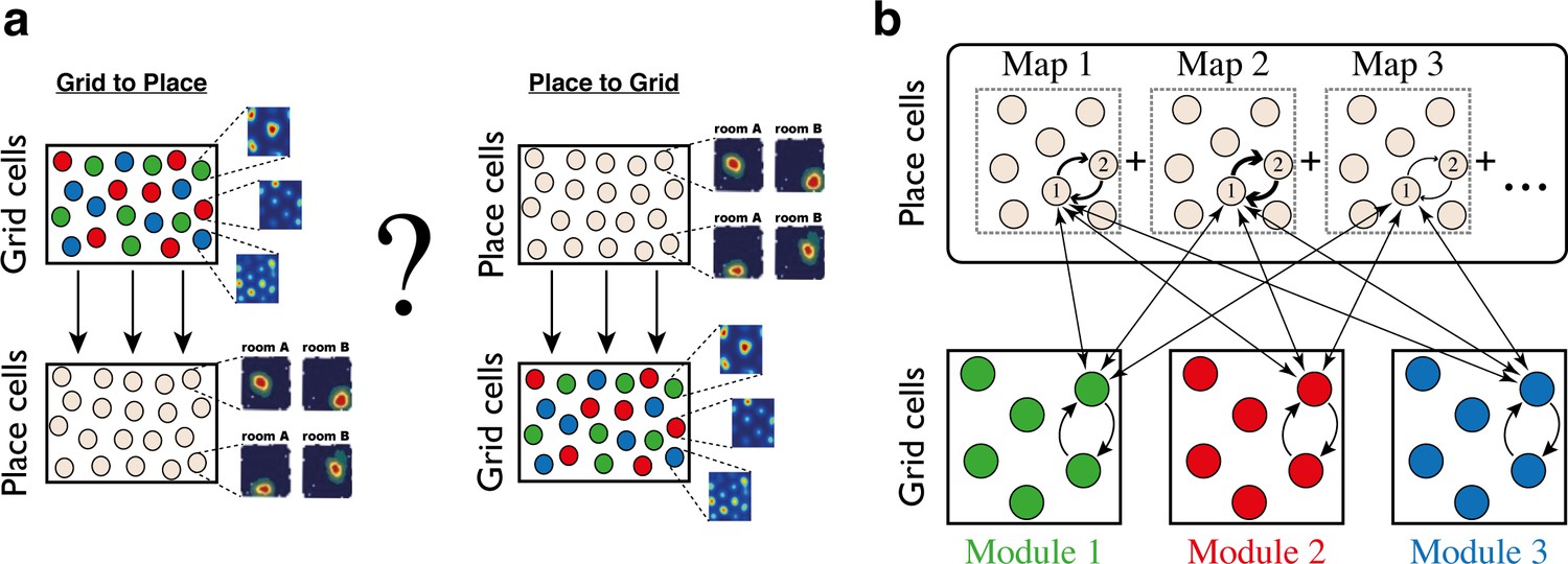
Schematic illustration: possible architectures of grid cell and place cell connectivity.
(a) Two hypotheses on connectivity, with hierarchical relationship between grid cells and place cells. Left: feed-forward connectivity from grid cells to place cells. Right: feed-forward connectivity from place cells to grid cells. Grid cells are color coded by their allocation to modules. Place cells exhibit global remapping between distinct environments (room A/room B) accompanied by grid cells realignment (not shown). (b) Schematic illustration of the model’s architecture: place cells and grid cells are bidirectionally coupled. Top: the strength of synaptic connectivity between a pair of place cells is a sum of map-specific contributions arising from the distinct maps. In each discrete map, the connectivity depends on the environment-specific spatial separation between the place cell receptive fields (arrow thicknesses for place cells #1 and #2). Bottom: grid cell modules are modeled as independent continuous attractors. Recurrent connectivity is identical in all modules. Straight arrows: the bi-directional connection between a grid cell and a place cell is proportional to the overlap between their receptive fields across the discrete maps.
Figure 2

Examples of simulation results, demonstrating joint persistent states of place cells and grid cells.
(a) One persistent state of the network (state 1). In each panel, cells are ordered according to their preferred firing locations in one environment. In each grid cell module, positions displaced by any integer multiple of the grid spacing correspond to the same cell, whereas distinct place cells span the whole extent of the environment. When cells are ordered according to their preferred firing locations in map #1 (left), a unimodal place cell bump is observed, and the distinct grid cell bumps of the three modules co-localize around the same spatial location. When the cells are ordered according to their preferred firing locations in a different map (middle - map #3 and right - map #6), the same place cell activities are scattered throughout the environment and do not resemble a unimodal activity bump. Furthermore, grid cell bumps do not necessarily co-localize around the same spatial location, as they independently realign. (b-c) Examples of persistent states (state 2 and 3), similar to (a) but representing positions in map #3 and in map #6 respectively. Note that here the activity of place cells seems scattered and grid cell bumps independently realign when cells are ordered according to their preferred firing locations in map #1.
Figure 3 with 5 supplements
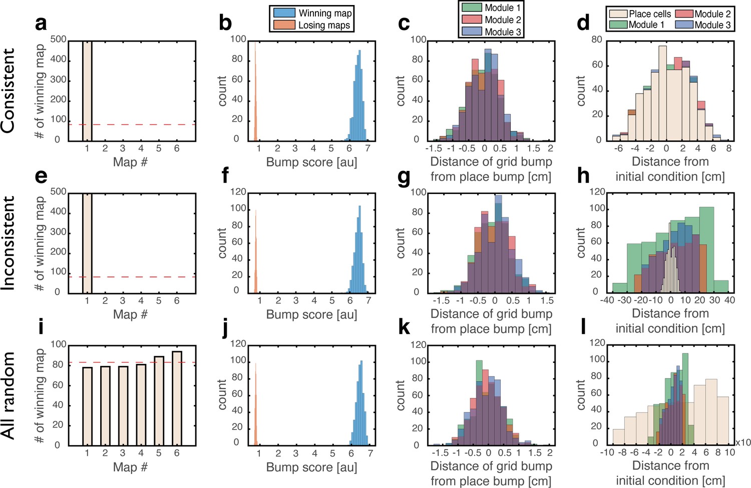
Quantitative mapping of the persistent states expressed by the joint network.
In all panels, the system is placed at 500 initial conditions of three types (a-d: ‘consistent’, e-h: ‘inconsistent’, i-l: ‘all random’). Its state is then analyzed after a 1 s delay period. (a-d) Results from the ‘consistent’ initial condition (the system is placed without loss of generality in map #1). (a) Histogram of winning map, defined as the map that achieved the highest bump score. Red dashed line: uniform distribution. (b) Histogram of place cell bump scores, obtained from the winning map (blue) and from an average on all other maps (‘Losing maps’, orange). (c) Histogram of distances between the measured spatial location of each grid cell bump and the place cell bump, evaluated in the coordinates of the winning map. (d) Histogram of distances traveled by the activity bumps from their initial condition, evaluated in the coordinates of the winning map. (e-h) Similar to (a-d) but for ‘inconsistent’ condition. (i-l) Similar to (a-d) but for ‘all random’ condition. The initial position was evaluated using the same algorithm used in (d,h) but in this case, where there were no initial bumps, the outcome depended on slight random variations in the initial condition and thus, effectively, the initial position was chosen randomly. Note that for all initial conditions the state of the system after the delay period corresponded to a single spatial map (b,f,j), and the place cell and grid cell representations are coordinated (c,g,k).
Figure 3—figure supplement 1
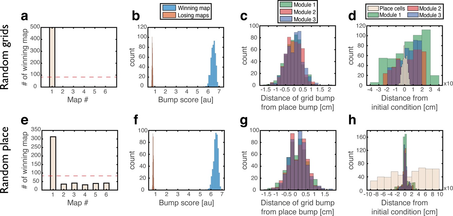
Analysis of persistent states following initial conditions of type (4).
(a-d) Similar to Figure 3a–d but for ‘Grid cells - random, Place cells - bump’ initial conditions: grid cells were initially set to have random rates, while place cells were set to encode a specific location. (e–h) Similar to Figure 3a–d but for ‘Place cells - random, Grid cells - bump’: grid cells were set to encode a specific location, and place cells were assigned with random rates.
Figure 3—figure supplement 2
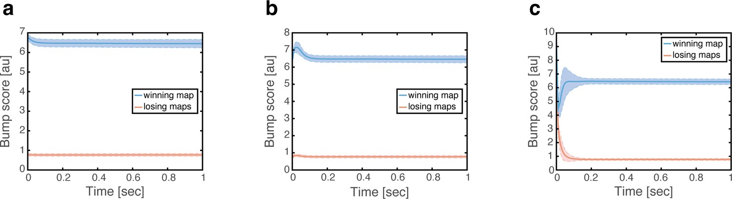
Bump score dynamics of persistent states.
(a) Bump score dynamics in the ‘consistent’ initial condition, corresponding to all realizations shown in Figure 3a–d. Error bars correspond to ±1 std. (b) Same as (a) but in the ‘inconsistent’ initial condition (same realizations as shown in Figure 3e–h). (c) Same as (a) but in the ‘all random’ initial condition (same realizations as shown in Figure 3i–l).
Figure 3—video 1
Dynamics under ‘consistent’ initial condition.
Firing rates of place cells (black) and grid cell modules (red, green, and blue) during a single 1 s simulation, in which the network was initialized in a ‘consistent’ state in map 1. Left: neurons are sorted according to firing locations in map 1. Right: neurons are sorted according to firing locations in map 5.
Figure 3—video 2
Dynamics under ‘inconsistent’ initial condition.
Firing rates of place cells (black) and grid cell modules (red, green, and blue) during a single 1 s simulation, in which the network was initialized in an ‘inconsistent’ state in map 1. Left: neurons are sorted according to firing locations in map 1. Right: neurons are sorted according to firing locations in map 6.
Figure 3—video 3
Dynamics under ‘all random’ initial condition.
Firing rates of place cells (black) and grid cell modules (red, green, and blue) during a single 1 s simulation, in which the network was initialized in an ‘all random’ state. Left: neurons are sorted according to firing locations in map 1. Right: neurons are sorted according to firing locations in map 4.
Figure 4 with 1 supplement
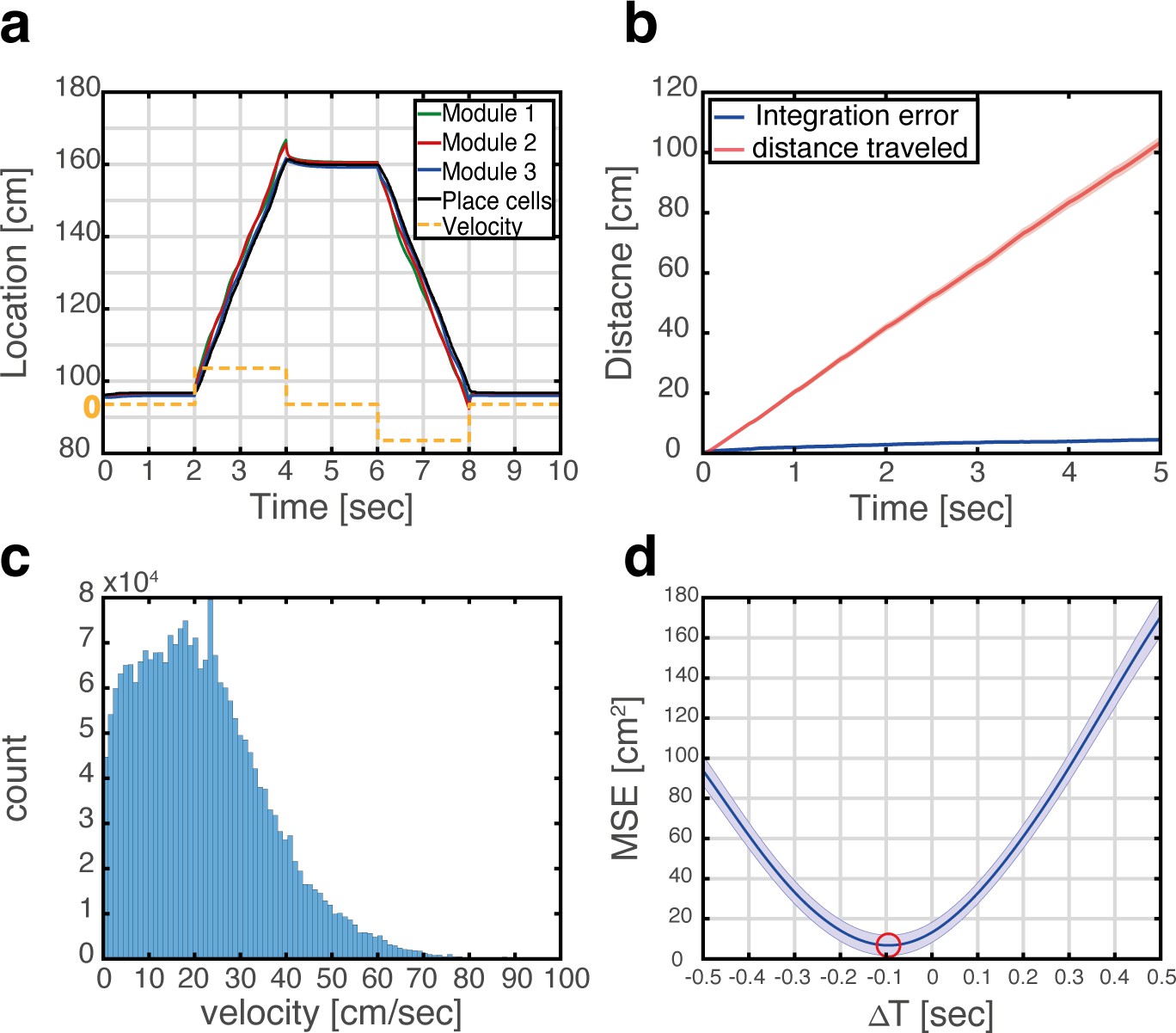
Velocity integration in grid cells can update the place cell representation.
(a) Readout of place cell bump location (black) while grid cell modules (green, red, and blue) integrate a velocity profile (dashed orange line). (b) Mean absolute distance between measured location of the place cell activity bump, and integrated velocity (blue), as a function of time. This quantity is compared with the total distance traveled by the place cell bump (red), which is much larger. Averaging was performed over 500 trajectories. In each trajectory velocity was randomly sampled every 0.5 s from an experimentally measured velocity distribution, which was obtained during foraging of a rat in an open-field environment (see panel c). Shaded error bars are 1.96 times the standard deviations obtained from each simulation, divided by the square root of the number of realizations (corresponding to a confidence interval of 95%). (c) Histogram of velocities measured experimentally during foraging of a rat in an open field environment (Hafting et al., 2005). (d) Mean squared displacement between positions represented by place cells and grid cells, when evaluated at varying time lags between the two measurements. Red circle marks the minimal MSE. The minimum MSE occurs at a negative time lag (~−100 ms), which indicates that the place cell representation lags behind the grid cell representation. Shaded error bars are 1.96 times the standard deviations obtained from each simulation, divided by the square root of the number of realizations (corresponding to a confidence interval of 95%).
Figure 4—figure supplement 1
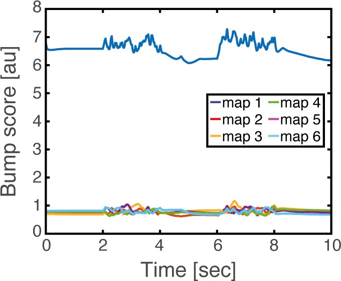
Bump score dynamics for each of the embedded maps, corresponding to the realization shown in Figure 4a.
Figure 5
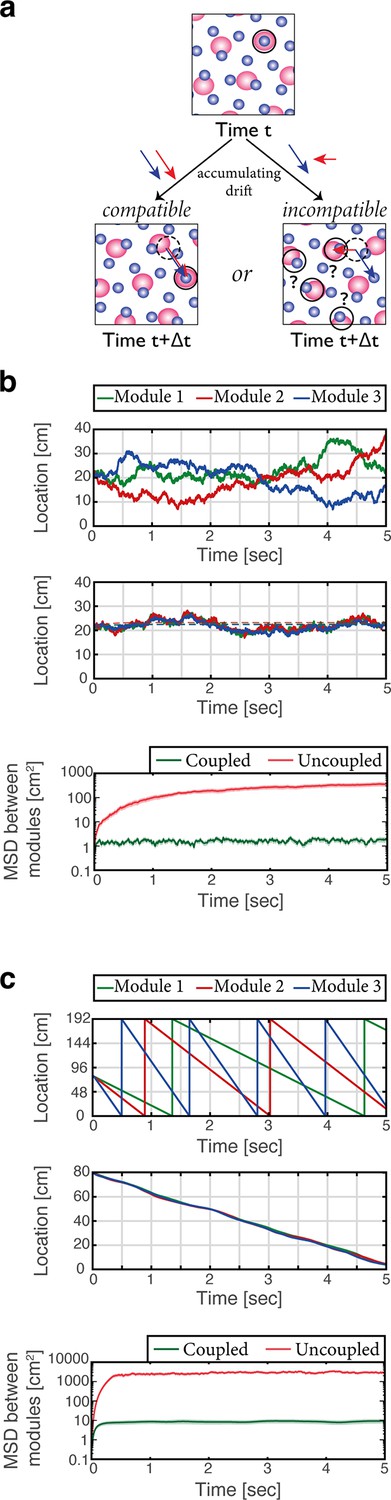
Place cells coordinate the representations of position in distinct grid cell modules.
(a) The need for coupling. Top panel: blue- and red-shaded areas represent schematically the posterior likelihood for the animal’s position in 2-d, obtained from the activity of all grid cells in module 1 (red) and module 2 (blue). Periodic colored blobs correspond to areas with high likelihood for the position, while blank areas correspond to low likelihood (note that since the blobs represent a decoded likelihood from the activity of all grid cells in the same module, they should not be confused with the spatial receptive fields of single cells). The position which is most likely given the joint activity in both modules is designated by a black circle. Bottom left: when noise-driven drifts in the two modules are identical (compatible drifts, blue and red arrows), the outcome is a shift in the represented position (original location marked by black dashed circle for reference). Bottom right: incompatible drifts in the two modules may result in abrupt jumps in the maximum-likelihood location (Burak, 2014; Mosheiff and Burak, 2019). (b) Examples of 1-d simulation results starting from a consistent initial condition showing grid cell module bump locations (green, red and blue) vs. time without (up) and with (middle) coupling between place cells and grid cells. Random accumulated drifts are driven by intrinsic neural noise, modeled as arising from Poisson spiking. Dashed lines in middle panel are generated from a non-noisy simulation for reference. Bottom: mean square displacement (MSD) between bump locations of distinct grid cell modules (averaged across all pairs and realizations of the stochastic dynamics) vs. time with (green) and without (red) coupling between place cells and grid cells, starting from a consistent initial condition. Shaded error bars are 1.96 times the standard deviations obtained from each simulation, divided by the square root of the number of realizations (corresponding to a confidence interval of 95%). (c) Similar examples (top, middle) and analysis (bottom) as in (b) but obtained from simulations in which drifts arise from incompatible velocity inputs provided to the distinct modules.
Figure 6
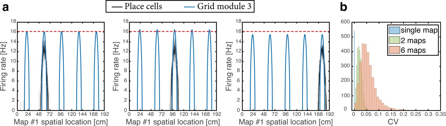
Spontaneously emerging variability of individual grid cell firing rates across firing fields.
(a) Simultaneous firing rates of place cells (black) and grid cells from one module (module #3, blue), shown at three different persistent states that represent periodic locations of module #3. Even though the same grid cells are active in all three locations, the amplitude of the grid cell activity bumps differ (compared with the red dashed line which shows the maximal grid cell firing rate achieved at the left example, for reference). Different place cells are active in the three examples, thus providing different quenched noise to the same grid cells in each case. (b) Histogram showing CV of maximal firing rate obtained from all individual grid cells across firing fields within a single environment, shown for networks with a single map (blue), two maps (green), and six maps (red).
Figure 7 with 4 supplements
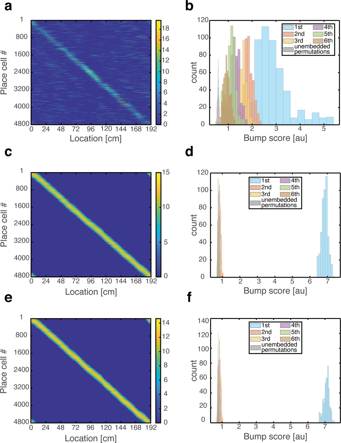
Emergence of persistent mixed states under depolarization but not under hyperpolarization of grid cells.
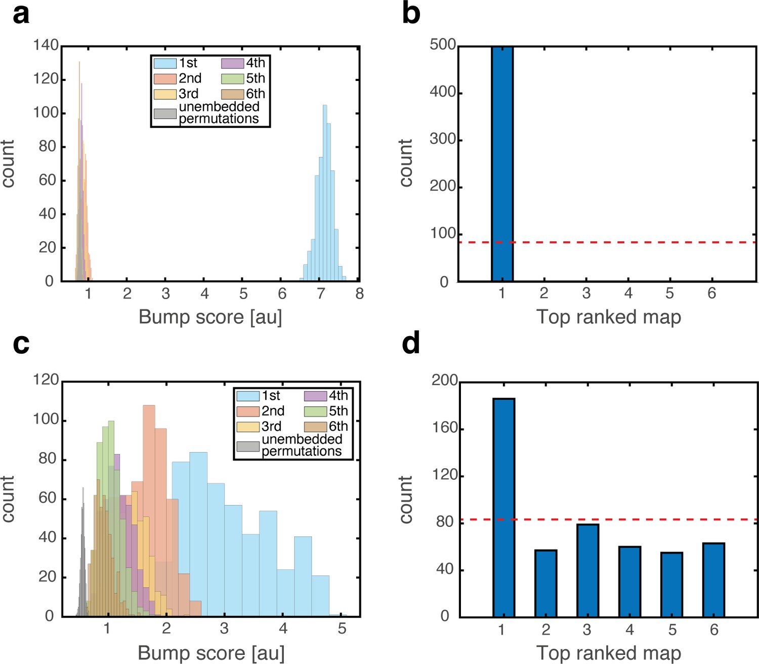
(a) Histogram showing bump score distributions for all embedded maps under grid cell hyperpolarization. In each simulation, the system is placed in a ‘consistent’ initial condition, and hyperpolarization is applied. Spatial maps are then ranked according to their bump score. Each color corresponds to a histogram over all bump scores from maps with specific rank, regardless of the map’s identity (this is identical to the analysis shown in Figure 3b,g,f except that here losing maps are separated into distinct histograms according to rank). Bump scores for random unembedded maps are shown in gray. (b) Distribution of identities of the top scored maps from (a). Dashed red line shows the uniform distribution. In all realizations, top ranked map is map #1. (c) Same as (a) under grid cell depolarization. Bump scores are lower than the winning scores in Figure 3b. Bump score distributions from differently ranked maps overlap, and all histograms exhibit significantly higher bump scores than those of unembedded maps (gray), indicating simultaneous expression of activity patterns from multiple embedded maps. (d) Same as (b) under grid cell depolarization.
Figure 7—figure supplement 1
Persistent mixed state examples, and maintenance of grid cell firing location but not firing rate under grid cell depolarization.
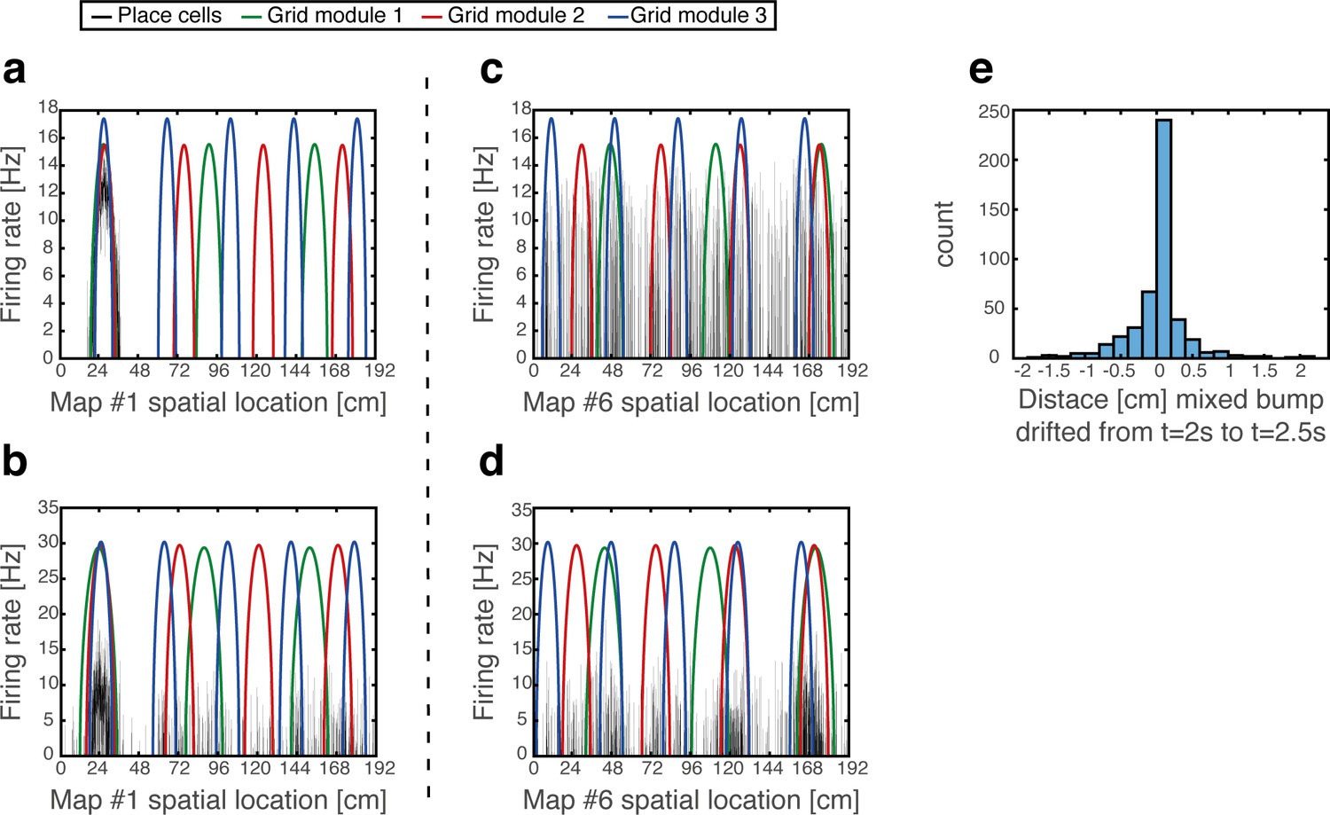
(a) Firing rates of place cells (black) and grid cells (different modules shown in green, red and blue), shown 2.25 s after starting from a ‘Consistent’ initial condition at a specific location (24 cm in map #1). (b) Same as (a) but under grid cell depolarization. Place cells exhibit scattered activity, yet they preserve dense activity around their original location from (a). Note that the grid cell activity patterns continue to match the original location in map #1, but grid cells increased their firing rate. (c–d) Same as (a–b) but observed in coordinates of map #6. Dense place cell activity can be seen around three locations (~48 cm,~120 cm and ~168 cm) under grid cell depolarization (d). Note that these locations overlap with locations in which multiple grid cell activity bumps overlap under the coordinates of map #6. (e) Analysis of persistence in the mixed state. Location of activity place cell bumps of winning maps was measured using the bump score as in Figure 3 (Methods), 2 s and 2.5 s after onset of depolarization. A histogram of the changes in the measured location within this period is shown, demonstrating that drifts in persistent mixed states are small. Out of 500 simulations, 29 simulations in which the identity of the winning map changed within this period are excluded from the histogram.
Figure 7—figure supplement 2

Bump score dynamics under grid cell hyperpolarization and depolarization.
(a) Bump score dynamics for each of the embedded maps and for unembedded maps (gray) under grid cell hyperpolarization, corresponding to the realizations shown in Figure 7a–b. Scores for all maps except map one overlap with the score of unembedded maps. Error bars correspond to ±1 std. (b) Same as (a) but showing only the winning map and an average over losing maps. Error bars correspond to ±1 std. (c) Same as (a), but under grid cell depolarization, corresponding to the realizations shown in Figure 7c–d. (d) Same as (b) but under grid cell depolarization.
Figure 7—figure supplement 3
Mixed states can be induced or suppressed by changing the connectivity between grid cells and place cells.
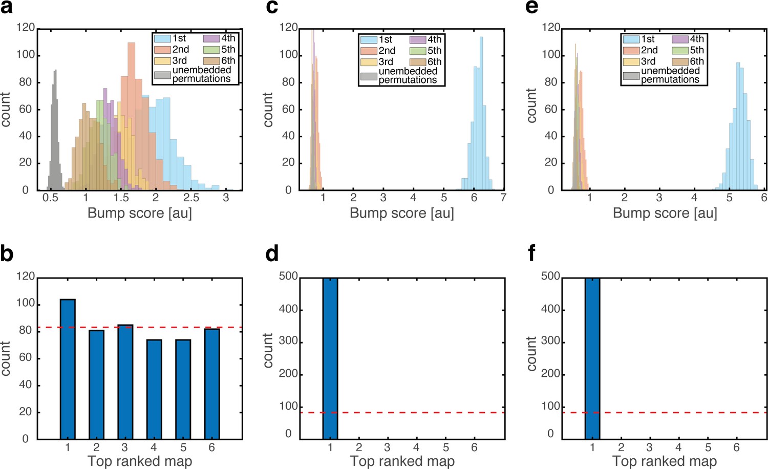
(a-b) Same analysis as Figure 7a–b but while doubling the bi-directional synaptic strengths between grid cells and place cells. Mixed states emerge under this manipulation, without grid cell depolarization. (c–d) Same as (a–b) but while selectively enhancing only the contribution to the connectivity associated with map #1. Mixed states do not emerge in this case. (e–f) Same as (c–d) but under grid cell depolarization. Although winning map bump score (cyan) is smaller than in Figure 3b, mixed states still do not emerge in this case.
Figure 7—video 1
Dynamics under grid cell depolarization.
Firing rates of place cells (black) and grid cell modules (red, green, and blue) during a single 2.5 s simulation (shown also in Figure 7—figure supplement 1a–d), in which the network was initialized in a ‘consistent’ state, followed after 10 ms by grid cell depolarization, which lasted until the end of the simulation. Left: neurons are sorted according to firing locations in map 1. Right: neurons are sorted according to firing locations in map 6.
Figure 8 with 2 supplements
Artificial remapping of place cells following depolarization, but not hyperpolarization of grid cells.
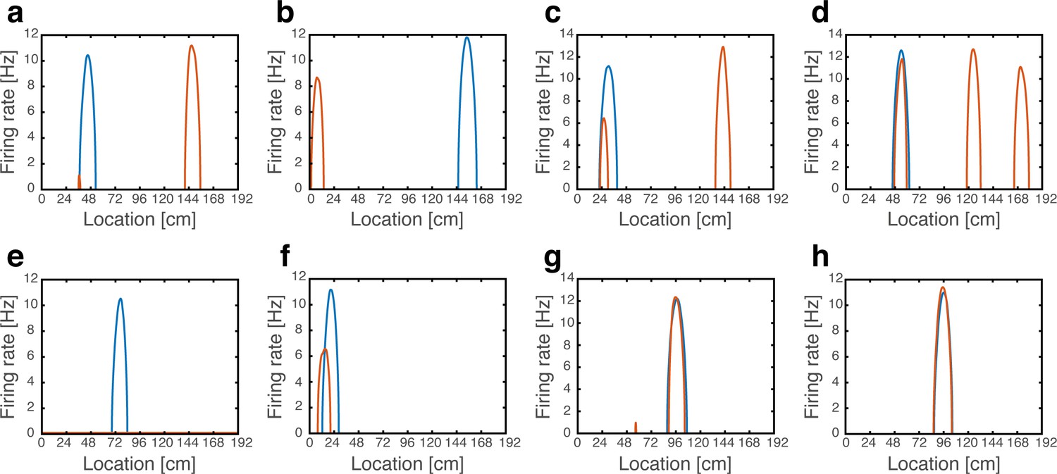
(a-g) Firing rate maps of seven representative place cells during locomotion without (blue) and with (orange) grid cell depolarization. Rate maps show that under grid cell depolarization place cells changed locations (a-b), acquired additional fields (c-d), turned off (e), rate remapped (f) or were unaffected (g). (h) Rate maps of a representative place cell without (blue) and with (orange) grid cell hyperpolarization.
Figure 8—figure supplement 1
Place cell population activity patterns observed while traversing the environment using path integration.
(a) Place cell firing rates vs. spatial location under grid cell depolarization and grid cell integration of velocity input that produces one complete cycle through the environment. Color bar: place cell firing rates [Hz]. Place cells exhibit uni-modal and continuous firing fields. Same result is obtained while traversing the environment with different velocities, direction, or number of cycles through the environment (not shown). (b) Similar analysis as in Figure 7a, showing the existence of mixed states throughout the process. Activity patterns were analyzed at 500 time points uniformly distributed across the cycle. (c–d) Same as (a–b) but without grid cell depolarization (control). (e–f) Same as (a–b) during grid cell hyperpolarization.
Figure 8—figure supplement 2
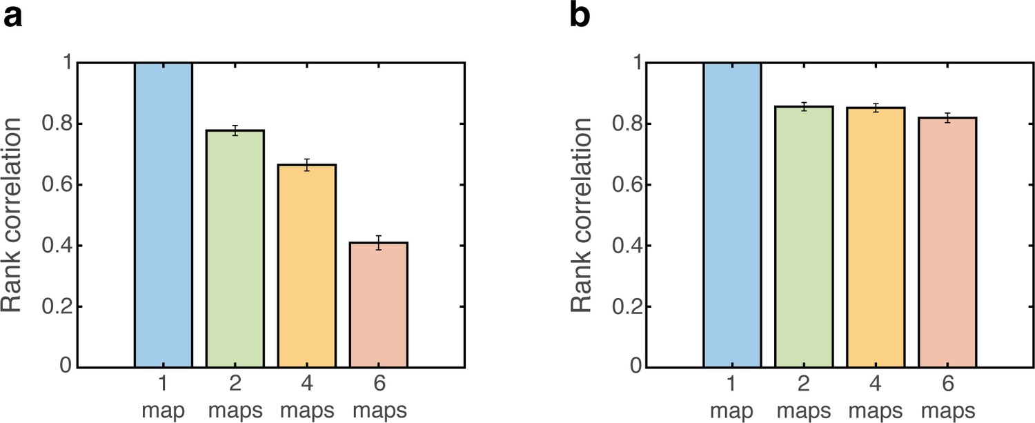
Altered firing rate relationship between individual grid fields is observed during grid cell depolarization.
(a) Spearman rank correlation before and after grid cell depolarization is shown for a varied number of embedded maps. Perturbation was applied persistently 10 ms after starting from a ‘consistent’ initial condition and grid cell rates were measured 100 ms afterwards. Rates were measured from 4800 realizations, uniformly distributed over all positions. Error bars are 1.96 times the standard deviations obtained from each simulation, divided by the square root of the number of realizations (corresponding to a confidence interval of 95%). (b) Same as (a) but under grid cell hyperpolarization.
Appendix 1—figure 1
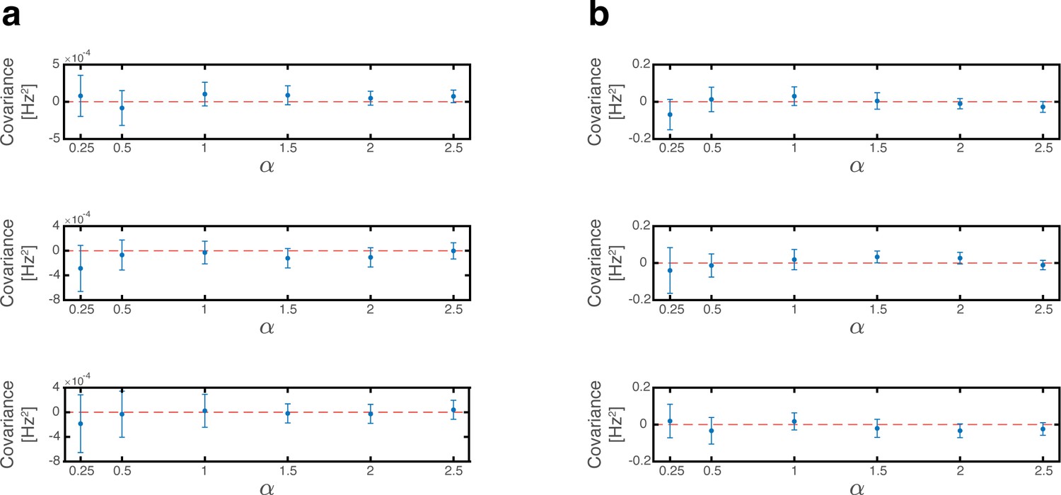
Covariances of place cell inputs across sub-populations vanish.
(a) Simulation results (blue dots) showing the covariance of place cell inputs arising from activities of pairs of different grid cell modules. A common scaling factor determines the number of place cells and grid cells in each module where was used throughout this manuscript. Red dashed lines show the zero-identity line for reference. Top: covariance between first and second modules. Middle: covariance between first and third modules. Bottom: covariance between second and third modules. Simulation results include 2000 random map realizations bootstrapped into 40 batches of 50 realizations to obtain multiple covariance measurements. Error bars are 1.96 times the standard deviations obtained from each simulation, divided by the square root of the number of realizations (corresponding to a confidence interval of 95%). (b) Same as (a) but for the covariance of place cell inputs arising from activities of place cells and each of the grid cell modules. Top: covariance between place cells and first grid cell module. Middle: covariance between place cells and second grid cell module. Bottom: covariance between place cells and third grid cell module.
Appendix 1—figure 2
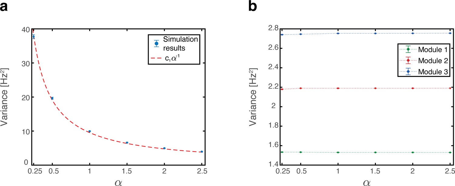
Variance of place cell inputs.
(a) Simulation results (blue dots) showing the variance of place cell inputs arising from place cell activities. A common scaling factor determines the number of place cells and grid cells in each module where was used throughout this manuscript. Simulation results include 2000 random map realizations bootstrapped into 40 batches of 50 realizations to obtain multiple variance measurements. Error bars are 1.96 times the standard deviations obtained from each simulation, divided by the square root of the number of realizations (corresponding to a confidence interval of 95%. Some error bars are too small to be visible). Dashed red line shows the curve with optimal fitted for reference, . (b) Same as (a) but for the variance of place cell inputs arising from grid cell activities.
Appendix 1—figure 3
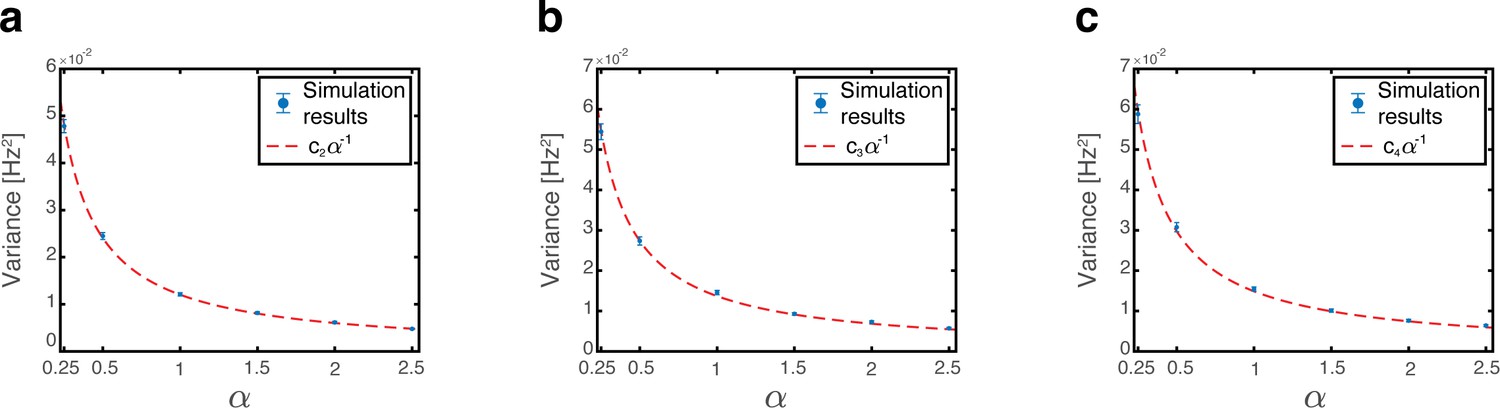
Variance of grid cell inputs.
(a) Simulation results (blue dots) showing the variance of grid module 1 inputs arising from place cell activities. A common scaling factor determines the number of place cells and grid cells in each module where was used throughout this manuscript. Simulation results include 2000 random map realizations bootstrapped into 40 batches of 50 realizations to obtain multiple variance measurements. Error bars are 1.96 times the standard deviations obtained from each simulation, divided by the square root of the number of realizations (corresponding to a confidence interval of 95%. Some error bars are too small to be visible). Dashed red line shows the curve with optimal fitted for reference, . (b) Same as (a) but for grid module 2. Dashed red line shows the curve with optimal fitted for reference, . (c) Same as (a) but for grid module 3. Dashed red line shows the curve with optimal fitted for reference, .
Appendix 1—figure 4
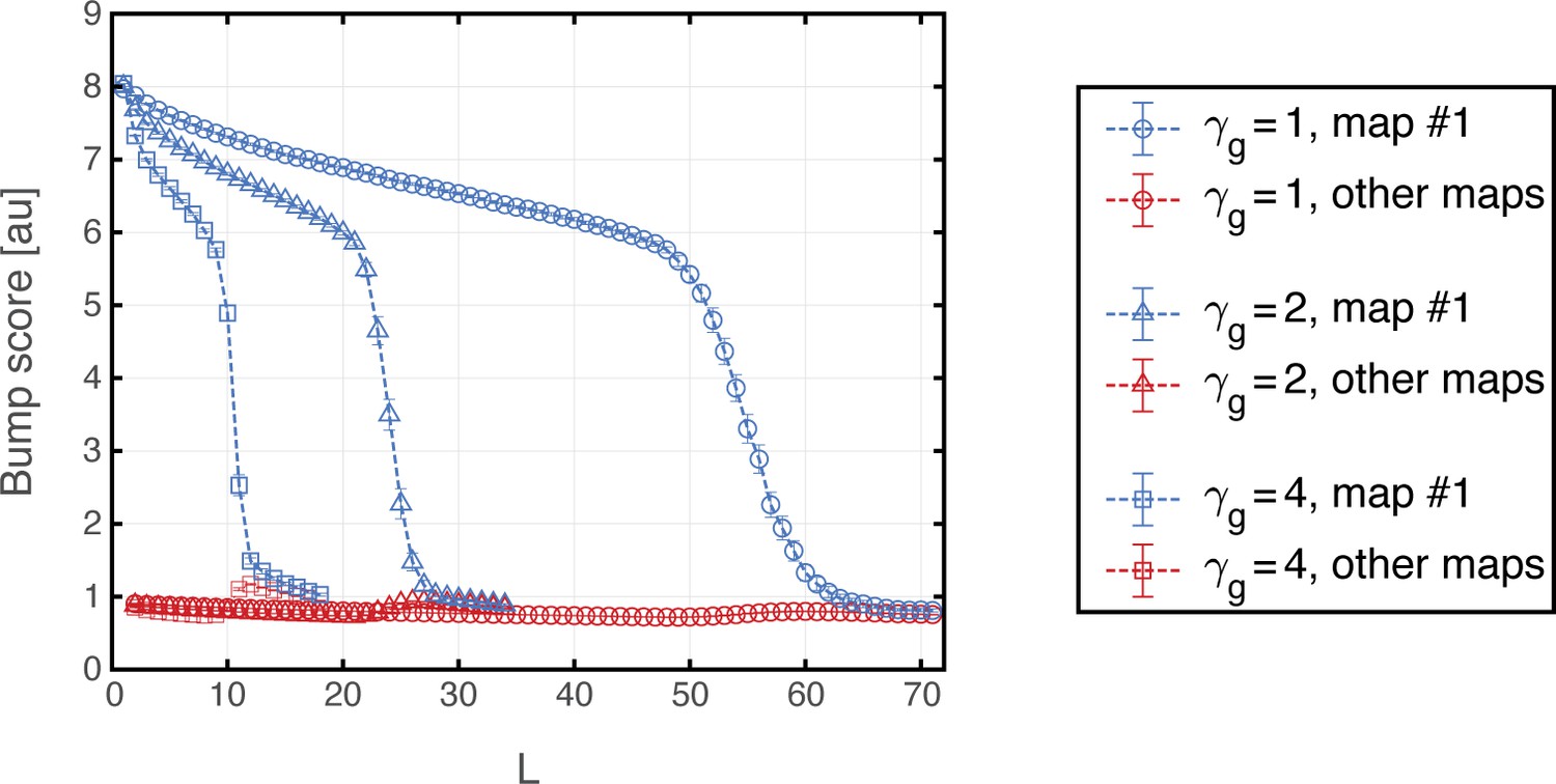
Capacity dependence on grid to place coupling parameter.
Bump score vs the total number of embedded maps for three different values of (circle, triangle and square) when starting from a ‘consistent’ initial condition in map #1. Blue curves show the bump score for map #1 and overlapping red curves show the average bump score for the rest of the embedded maps (whenever ). Each plotted value is the average bump score obtained from 100 randomly chosen realizations for each specific value of (and including 5 randomly chosen initial conditions within each realization). Error bars are 1.96 times the standard deviations obtained from each simulation, divided by the square root of the number of realizations (corresponding to a confidence interval of 95%. Some error bars are too small to be visible).
Tables
Table 1
| Parameter | Value | Units |
|---|---|---|
-
*In all Figures we simulated the same networks using , except for Figure 6b (where was also set to 1 and 2), and Figure 8—figure supplement 2 (where was also set to 1, 2 and 4).
Additional files
Download links
A two-part list of links to download the article, or parts of the article, in various formats.
Downloads (link to download the article as PDF)
Open citations (links to open the citations from this article in various online reference manager services)
Cite this article (links to download the citations from this article in formats compatible with various reference manager tools)
A theory of joint attractor dynamics in the hippocampus and the entorhinal cortex accounts for artificial remapping and grid cell field-to-field variability
eLife 9:e56894.
https://doi.org/10.7554/eLife.56894


