Localized inhibition in the Drosophila mushroom body
- Department of Biomedical Science, University of Sheffield, United Kingdom
- Neuroscience Institute, University of Sheffield, United Kingdom
- Centre for Neural Circuits and Behaviour, University of Oxford, United Kingdom
Figures
Figure 1 with 1 supplement

Spatially restricted responses to electric shock in APL.
(A) Diagrams of regions used to quantify APL activity in (B–C). (B) APL responses to electric shock (left) or the odor isoamyl acetate (right) in the regions defined in (A), in 474-GAL4 > GCaMP6f flies. Traces show mean ± SEM shading. Electric shock trace is the average of 3 shocks with 12 s between onset of each shock. Horizontal black lines show timing of electric shock (1.2 s) or odor (5 s). (C) Mean ∆F/F during the intervals shaded in panel (B). ## p<0.01, ### p<0.001, one-sample Wilcoxon test vs. null hypothesis (0) with Holm-Bonferroni correction for multiple comparisons. *p<0.05, ***p<0.001, Friedman test with Dunn’s multiple comparisons test for each group (V, H, S, and γ) against each other. n, given as # neurons (# flies): electric shock, 19 (15); odor, 13 (11).
-
Figure 1—source data 1
Source data for Figure 1C.
- https://cdn.elifesciences.org/articles/56954/elife-56954-fig1-data1-v2.xlsx
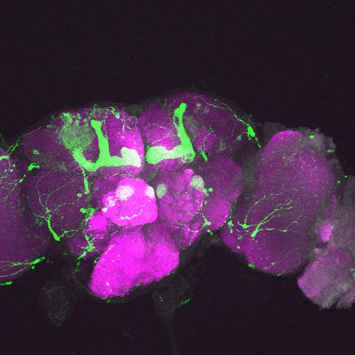
Figure 1—figure supplement 1
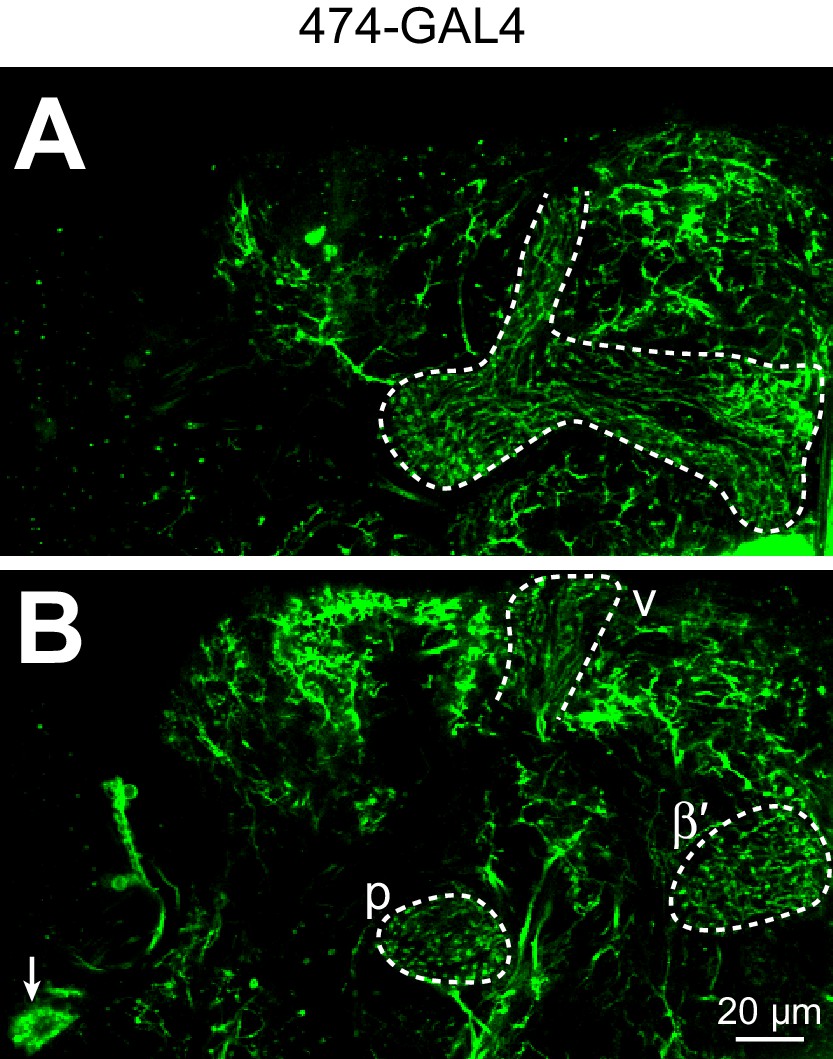
Expression pattern of 474-GAL4.
Individual z-slices of 474-GAL4 > UAS-CD8::GFP (unfixed brain imaged on two-photon). (A) APL in mushroom body lobes (dashed white outline). (B) APL in the anterior peduncle (p), tip of the vertical lobe (v), and tip of the β′ lobe (dashed white outlines) and the APL cell body (arrow). A and B are 18 µm apart. APL is obscured in a full z-projection due to fluorescence from non-APL neurons. Note the typical morphology of APL with neurites running largely parallel to Kenyon cells. A complete z-projection of 474-GAL4’s expression pattern is available at http://www.columbia.edu/cu/insitedatabase/adultbrain/IT.0474.jpg (Silies et al., 2013) (Grueber and Clandinin, personal communication).
Figure 2 with 1 supplement
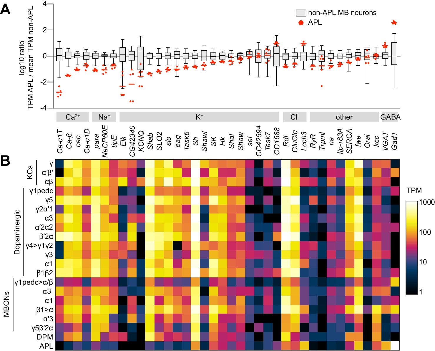
Low expression of voltage-gated Na+ and Ca2+ channels in APL.
(A) Expression levels of GABAergic markers and various Na+, Ca2+, K+, Cl- and other channels, in APL compared to non-APL mushroom body neurons, normalized to the mean of non-APL neurons. Box plots show the distribution of expression levels in non-APL MB neurons (whiskers show full range), using the average of log10(TPM) across biological replicates for each type. Red dots show five biological replicates of APL; red line shows the mean APL expression level. Genes are grouped by type and sorted by fold difference in APL expression relative to non-APL MB neurons. Data from Aso et al., 2019. TPM, transcripts per million. (B) Heat map of TPM counts (log scale) for all genes shown in (A), for all 21 cell types.
-
Figure 2—source data 1
Source data for Figure 2.
- https://cdn.elifesciences.org/articles/56954/elife-56954-fig2-data1-v2.zip
Figure 2—figure supplement 1
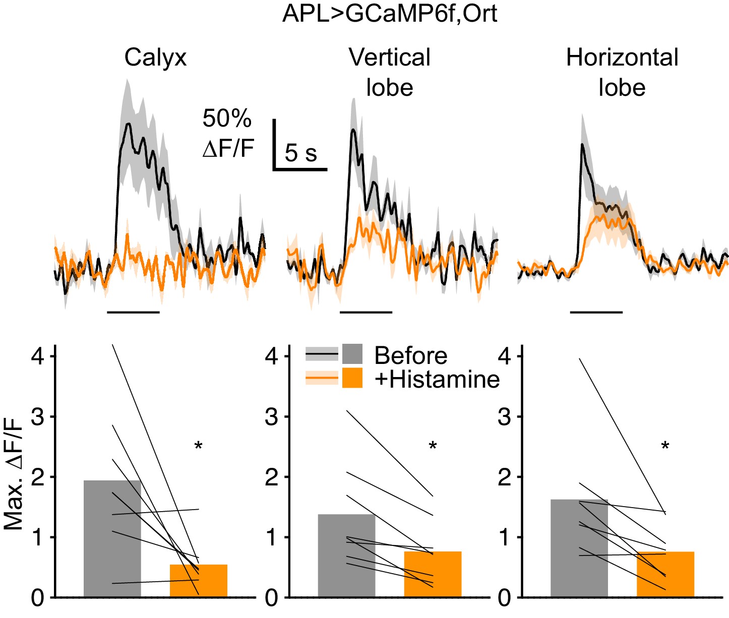
When APL expresses Ort, histamine reduces odor-evoked Ca2+ influx in APL.
Traces (mean ± SEM shading) show APL responses to isoamyl acetate (horizontal bars) before (black) and after (orange) bath-applying 2 mM histamine, in flies expressing GCaMP6f and the histamine-gated Cl- channel Ort in APL, driven by NP2631-GAL4/GH146-FLP. Graphs show maximum ∆F/F (same colors as traces). Bars show mean, thin lines show paired data (same hemisphere before and after histamine). *p<0.05, paired t-test or Wilcoxon test. The residual GCaMP6f response most likely reflects calcium influx through nAChRs (cholinergic input to APL when APL is blocked by histamine would be much higher due to increased KC activity: Apostolopoulou and Lin, 2020). Apparent differences in effect size in different parts of APL might reflect differential localization of Ort or differential penetration of histamine into the brain. Note that when APL does not express Ort, histamine has no effect on Kenyon cell odor responses (Apostolopoulou and Lin, 2020) and thus is unlikely to non-specifically affect APL odor responses.
-
Figure 2—figure supplement 1—source data 1
Source data for Figure 2—figure supplement 1.
- https://cdn.elifesciences.org/articles/56954/elife-56954-fig2-figsupp1-data1-v2.xlsx
Figure 3

Activating subsets of Kenyon cells only activates the corresponding lobe of APL.
(A) Time-averaged images of APL in a cross-section of the lower vertical lobe (dotted line in diagram) at room temperature (<25 °C) vs. heated (>30 °C). Activating α′β′ Kenyon cells expressing 0853-GAL4-driven dTRPA1 activates the α′ lobe, but not the α lobe, of APL. APL expresses GCaMP3 driven by GH146-QF. (B) Example responses to heating (black), by the α′ (red) and α (blue) lobes in the same APL recording. (C) ∆F/F for the α′ (red) and α (blue) lobes plotted against temperature. Each trace representing one recording forms a loop: it rises as the fly is heated (thick lines) and falls down a different path as the fly is cooled (thin lines). (D–F) As for (A–C) except activating αβ and γ Kenyon cells (mb247-GAL4 > dTRPA1) drives activity in the α, but not the α′ lobe of APL. (G,H) As for (C) and (F) except activating αβ Kenyon cells with c739-GAL4 (G) or NP3061-GAL4 (H). (I) Maximum ∆F/F between 30 °C and the peak temperature, summarizing data from (C,F–H). Lines indicate the same APL recording. *p<0.05, paired t-test with Holm-Bonferroni multiple comparisons correction. n (# flies), left to right: 5, 5, 5, 6. The expression patterns of mb247-GAL4, c739-GAL4, NP3061-GAL4 and GH146-QF were described previously (Potter et al., 2010; Qin et al., 2012; Zhou et al., 2019). The expression pattern of 853-GAL4 is available at http://www.columbia.edu/cu/insitedatabase/adultbrain/IT.0853.jpg.
-
Figure 3—source data 1
Source data for Figure 3I.
- https://cdn.elifesciences.org/articles/56954/elife-56954-fig3-data1-v2.xlsx
Figure 4
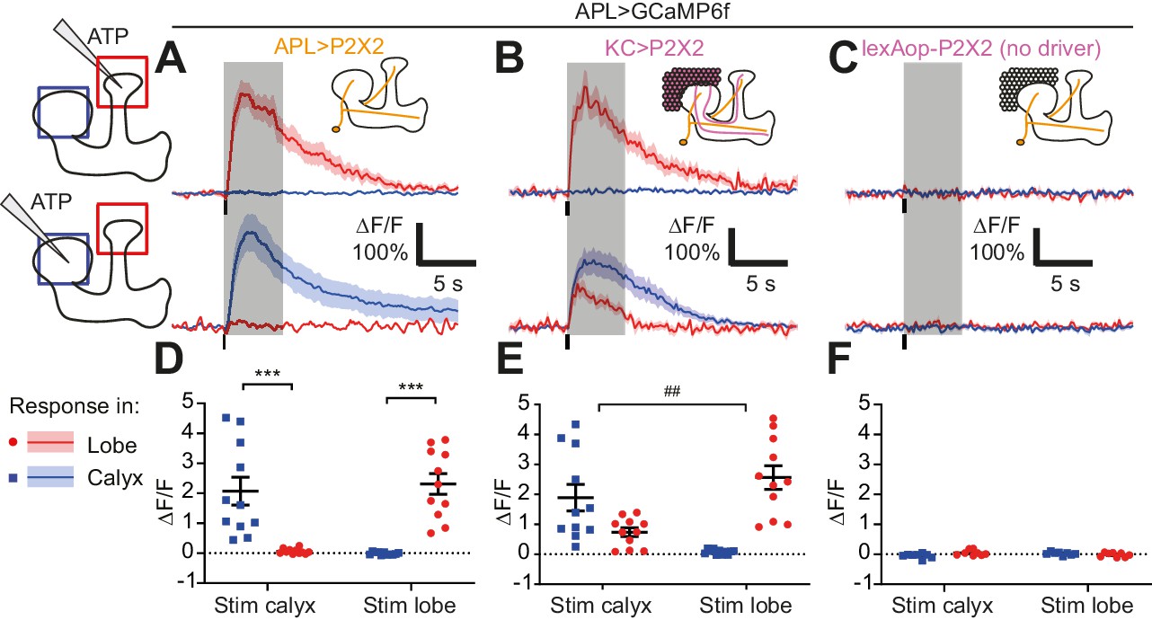
Activity in the APL neuron is spatially restricted.
(A–C) Response of APL in the vertical lobe (red) or calyx (blue) to pressure ejection of 1.5 mM ATP (100 ms pulse, 12.5 psi) in the lobe or calyx, to stimulate APL (A), KCs (B), or negative control flies with lexAop-P2X2 but no LexA driver (C). Schematics show ROIs where responses were quantified (red/blue squares), and where ATP was applied (pipette symbol). Traces show mean ± SEM shading. Vertical lines on traces show time of ATP application; gray shading shows 5 s used to quantify response in (D–F). GCaMP6f and/or P2X2 expressed in APL via intersection of NP2631-GAL4 and GH146-FLP. P2X2 expressed in KCs via mb247-LexA. See Supplementary file 1 for full genotypes. (D–F) Mean ∆F/F from (A–C), when stimulating APL (D), KCs (E), or negative controls (F). Error bars show SEM. n, given as # neurons (# flies): (A,D): 11 (9); (B,E): 11 (7); (C,F) 8 (4). ***p<0.001, t-tests with Holm Sidak multiple comparisons correction. ## p=0.004, paired t-test: the ratio of (response in unstimulated site)/(response in stimulated) site is higher for calyx stimulation than lobe stimulation.
-
Figure 4—source data 1
Source data for Figure 4D–F.
- https://cdn.elifesciences.org/articles/56954/elife-56954-fig4-data1-v2.xlsx
Figure 5 with 1 supplement
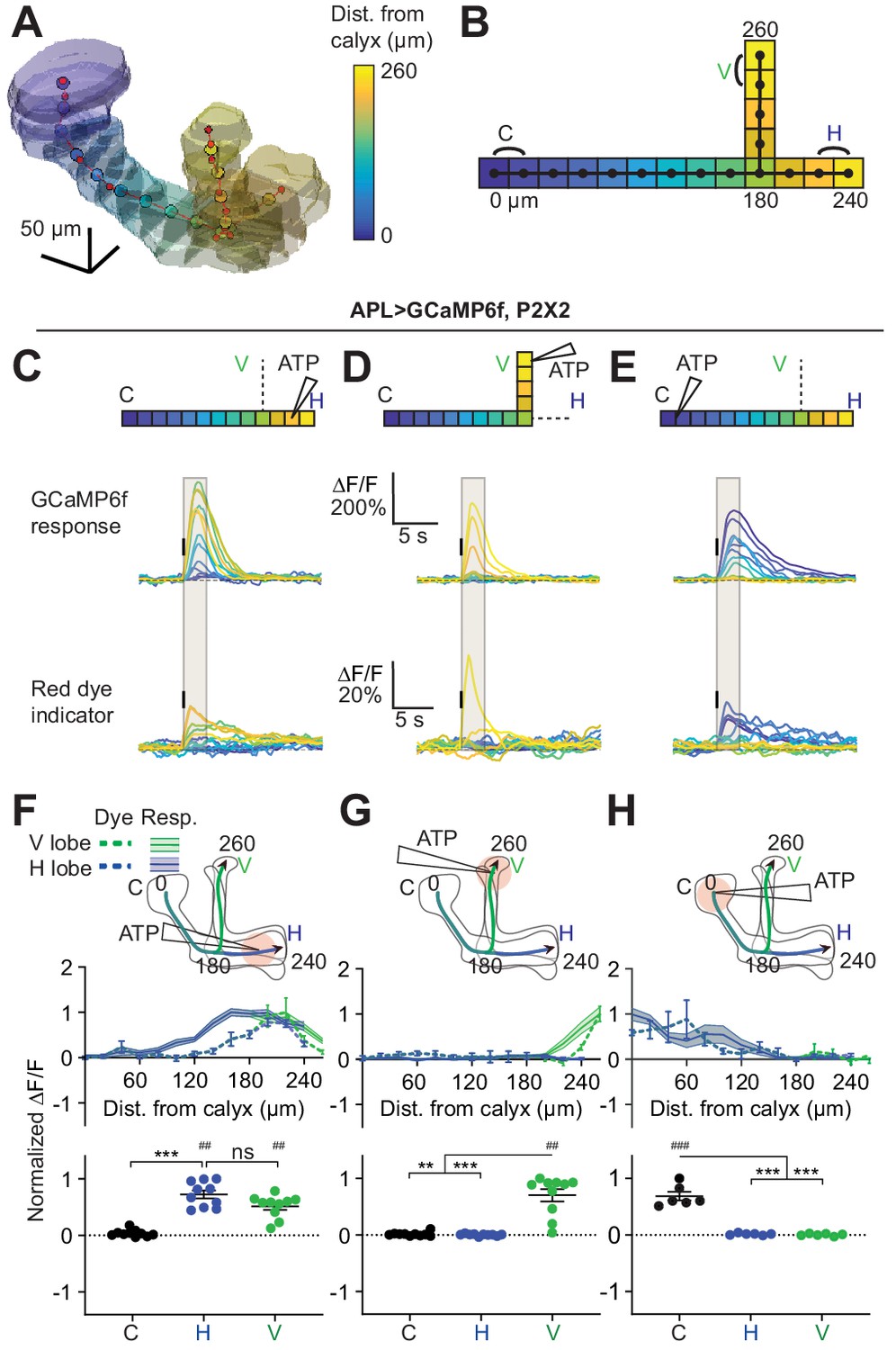
Quantification of activity spread in APL.
(A) 3D visualization of an example mushroom body manually outlined using mb247-dsRed as an anatomical landmark. The backbone skeleton is shown as a red line passing through the center of each branch of the mushroom body, manually defined by the red dots. Evenly spaced nodes every 20 µm on the backbone subdivide the mushroom body into segments, here color-coded according to distance from the dorsal calyx (scale on right). (B) Schematic of the ‘standard’ backbone with distances (µm) measured from the dorsal calyx. Color code as in panel A. In this and later figures, signals are quantified using the two outermost segments of the calyx (C, black), vertical lobe (V, green), and horizontal lobe (H, blue), as shown here. (C–E) Traces show the time course of the response in each segment of APL, averaged across flies, when stimulating APL with 0.75 mM ATP (10 ms puff at 12.5 psi) in the horizontal lobe (C), vertical lobe (D), or calyx (E), in VT43924-GAL4.2>GCaMP6f,P2X2 flies. Upper panels: GCaMP6f signal. Lower panels: Red dye signal. The baseline fluorescence for the red dye signal comes from mb247-dsRed. Color-coded backbone indicates which segments have traces shown (dotted lines mean the data is omitted for clarity; the omitted data appear in panels F–H). Gray shading shows the time period used to quantify ∆F/F in (F–H). Vertical black lines indicate the timing of ATP application. (F–H) Mean response in each segment (∆F/F averaged over time in the gray shaded period in C–E). The x-axis shows distance from the calyx (µm) along the backbone skeleton in the diagrams, and the color of the curves matches the vertical (green) and horizontal (blue) branches of the backbone. Solid lines with error shading show GCaMP responses; dotted lines with error bars show red dye. The responses in each panel were normalized to the highest responding segment (upper panels) or data point (lower panels). Error bars/shading show SEM. n, given as # neurons (# flies): (C, F, D, G) 10 (6), (E, H) 6 (4). ## p<0.01, ### p<0.001, one-sample Wilcoxon test or one-sample t-test, vs. null hypothesis (0) with Holm-Bonferroni correction for multiple comparisons. **p<0.01, ***p<0.001, Friedman test with Dunn’s multiple comparisons test or repeated measures one-way ANOVA with Holm-Sidak’s multiple comparisons test, comparing the stimulated vs the unstimulated sites. See Supplementary file 2 for detailed statistics.
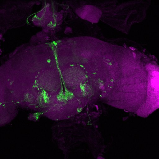
Figure 5—figure supplement 1
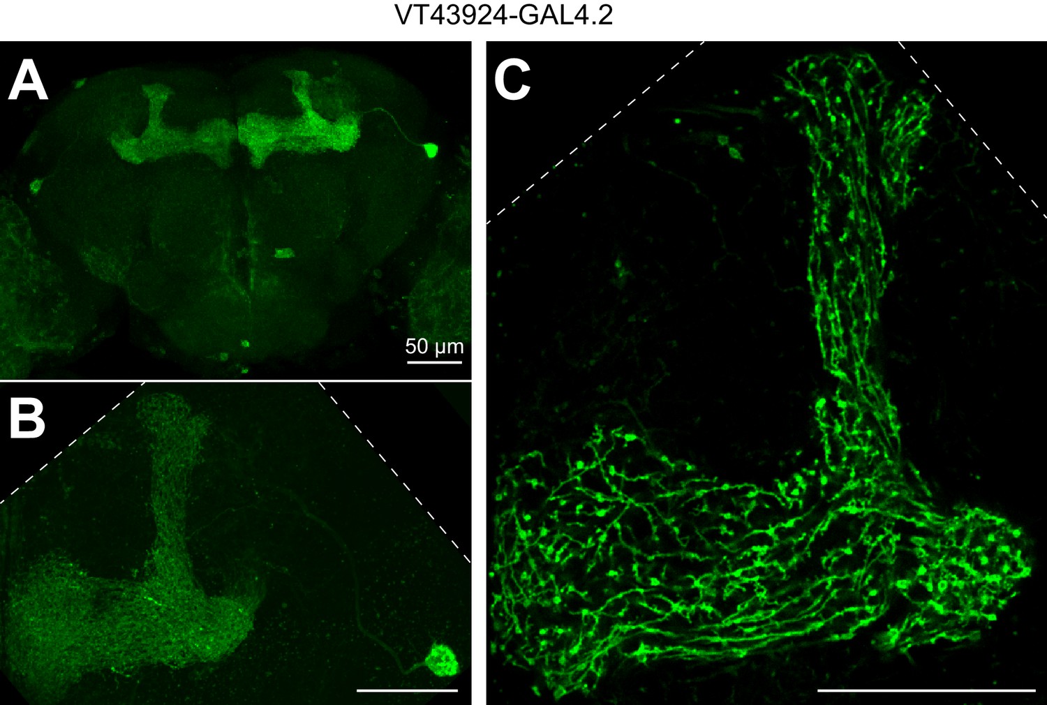
Expression pattern of VT43924-GAL4.2.
(A) Maximum intensity projection of confocal image of VT43924-GAL4.2-SV40 > UAS-CD8::GFP. (B) As in A, but zoomed in on a single APL (unfixed brain imaged on two-photon; calyx is less visible compared to A because the tissue is not fixed and cleared). (C) Same brain as B, single optical plane zoomed in to show fine structure of APL in the lobes. Scale bars, 50 µm. Dashed lines show the edge of the field of view.
Figure 6
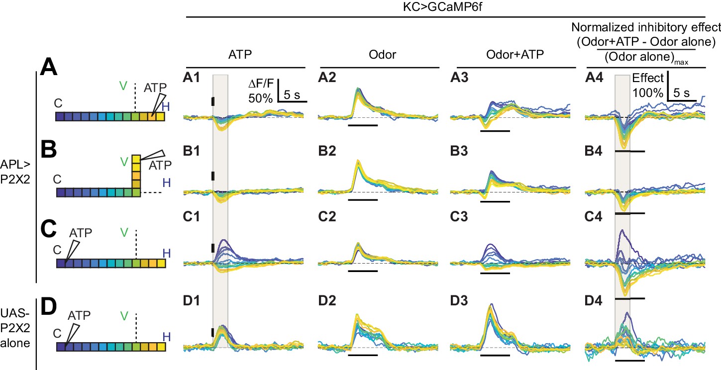
Time courses of APL’s inhibitory effect on KC activity.
Traces show the time course of the response in each segment of KCs, averaged across flies, when stimulating APL with 0.75 mM ATP (10 ms puff at 12.5 psi) in the horizontal lobe (A), vertical lobe (B), or calyx (C) in VT43924-GAL4.2>P2X2, mb247-LexA > GCaMP6f flies (no ATP stimulation in column 2). (D) shows responses in negative control flies (UAS-P2X2 alone). Columns 1–3 show responses of KCs to: (A1–D1) activation of the APL neuron by ATP, (A2–D2) the odor isoamyl acetate, (A3–D3) or both. (A4–D4) Normalized inhibitory effect of APL neuron activation on KC responses to isoamyl acetate (i.e. (column 3 - column 2)/(maximum of column 2)). The color-coded backbone indicates which segments have traces shown (dotted lines mean the data is omitted for clarity; the omitted data appear in Figure 7). Vertical and horizontal bars indicate the timing of ATP and odor stimulation, respectively. Gray shading in panels A1-D1 and A4-D4 indicate the intervals used for quantification in Figure 7 A2–C2 and A4–C4, respectively. The data in D1-D4 is quantified in Figure 7—figure supplement 2. n, given as # neurons (# flies): (A1–A4, B1–B4) 10 (9), (C1–C4) 9 (8), (D1–D4) 5 (3). Scale bar in A1 applies to columns 1–3; scale bar in A4 applies to column 4.
Figure 7 with 2 supplements
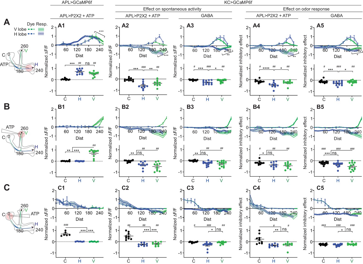
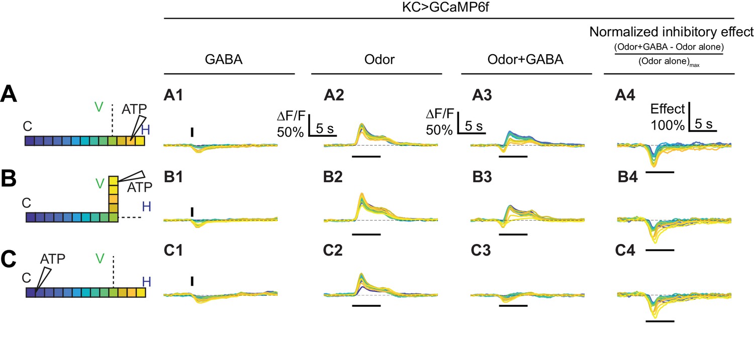
Quantification of the inhibitory effect of GABA or the APL neuron on KC activity.
Rows: Local application of ATP (0.75 mM) or GABA (7.5 mM) in the horizontal lobe (A1–A5), vertical lobe (B1–B5) or calyx (C1–C5). Columns: Column 1: APL’s response to ATP stimulation (A1–C1) in VT43924-GAL4.2>GCaMP6f,P2X2 flies, repeated from Figure 5 for comparison. Columns 2–3: KC responses to local activation of APL by ATP (A2–C2) or to GABA application (A3–C3). Columns 4–5: Normalized inhibitory effect of APL activation (A4–C4) or GABA application (A5–C5) on KC responses to isoamyl acetate. Genotypes: for ATP (columns 2,4): VT43924-GAL4.2>P2X2, mb247-LexA > GCaMP6f; for GABA (columns 3,5): OK107-GAL4 > GCaMP6f. Data shown are mean responses in each segment (averaged over time in the gray shaded periods in Figure 6). The x-axis (‘Dist’) shows distance from the calyx (µm) along the backbone skeleton in the diagrams (left), and the color of the curves matches the vertical (green) and horizontal (blue) branches of the backbone. Solid lines with error shading show GCaMP responses; dotted lines with error bars show red dye. The responses were normalized to the segment (upper panels) or data point (lower panels) with the largest absolute value across matching conditions (columns 2+3, or columns 4+5). The baseline fluorescence for the red dye comes from bleedthrough from the green channel; only trials without odour were used for red dye quantification, in these trials, the change in green bleedthrough (~10–40%) is negligible compared to the increase in red signal (150–300%). Error bars/shading show SEM. n, given as # neurons (# flies): (A1, B1) 10 (6), (C1) 6 (4), (A2, A4, B2, B4) 10 (9), (C2, C4) 9 (8) (A3, A5, B3, B5) 13 (8), (C3, C5) 11 (6). # p<0.05 ### p<0.001, one-sample Wilcoxon test, or one-sample t-test, vs. null hypothesis (0) with Holm-Bonferroni correction for multiple comparisons. *p<0.05, ***p<0.001, Friedman test with Dunn’s multiple comparisons test, or repeated-measures one-way ANOVA with Holm-Sidak multiple comparisons test, comparing the stimulated site vs. the unstimulated sites. Diagonal brackets in (A1–A5), paired t-test or Wilcoxon test comparing the response at segment 200 vs. 260 on the vertical branch. See Supplementary file 2 for detailed statistics.
-
Figure 7—source data 1
Source data for Figure 7 and Figure 7—figure supplement 2.
- https://cdn.elifesciences.org/articles/56954/elife-56954-fig7-data1-v2.xlsx
Figure 7—figure supplement 1
Time courses of GABA’s effect on KC activity.
Rows: Local application of GABA (7.5 mM) in the horizontal lobe (A1–A2), vertical lobe (B1–B2) or calyx (C1–C2). Columns: Responses of KCs to GABA application (A1–C1), the odor isoamyl acetate (A2–C2), or both (A3–C3). (A4–C4) Normalized inhibitory effect of GABA application on KC responses to isoamyl acetate. Traces show the time course of the response in each segment of KCs, averaged across flies. Color-coded backbone indicates which segments have traces shown (dotted lines mean the data is omitted for clarity; the omitted data appear Figure 7). Vertical and horizontal bars indicate the timing of GABA and odor stimulation, respectively.
Figure 7—figure supplement 2
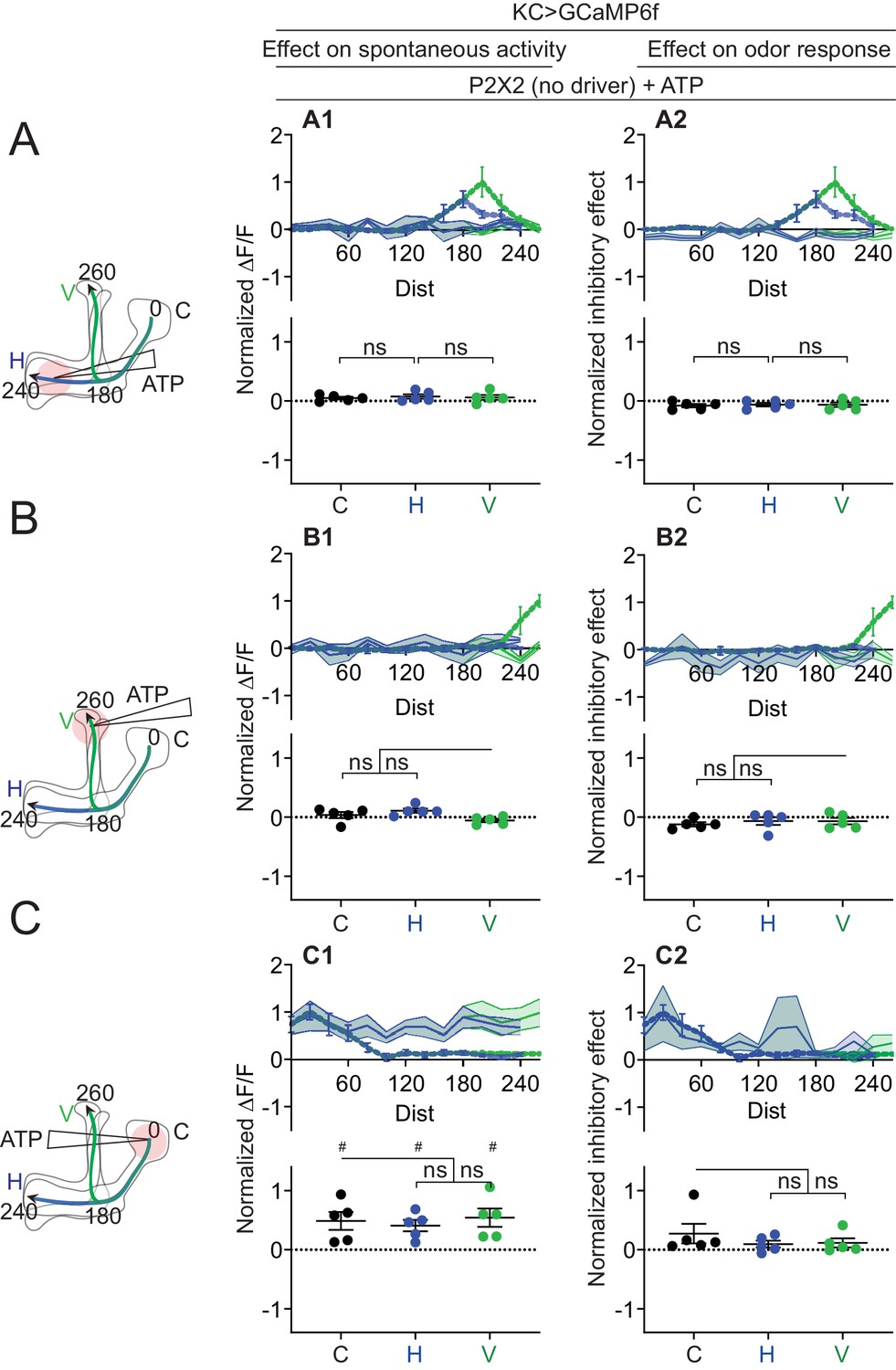
Quantification of effect of ATP on negative control (UAS-P2X2 only).
Rows: Local application of ATP (0.75 mM) in the horizontal lobe (A1–A2), vertical lobe (B1–B2) or calyx (C1–C2). Columns: KC responses to APL activation by ATP (A1–C1), or the normalized inhibitory effect of APL neuron activation on KC responses to isoamyl acetate (A2–C2). Data shown are mean responses in each segment (averaged over time in the gray-shaded periods in Figure 6). The color of the curves matches the vertical (green) and horizontal (blue) lobular branches depicted in the schematics shown on the left. The responses were normalized to the segment (upper panels) or data point (lower panels) with the largest absolute value in the corresponding experimental conditions (columns 2 and 3 in Figure 7 for column 1; columns 4 and 5 in Figure 7 for column 2). N: five neurons, three flies. # p<0.05, one-sample t-test, vs. null hypothesis (0) with Holm-Bonferroni correction for multiple comparisons. ns, p>0.05, one-way ANOVA with Holm-Sidak’s multiple comparisons test, comparing the stimulated site vs. the unstimulated sites. Paired t-test comparing the response at segment 200 vs. 260 on the vertical branch gives p = 0.2218 (A1), p = 0.9397 (A2).
Figure 8 with 4 supplements
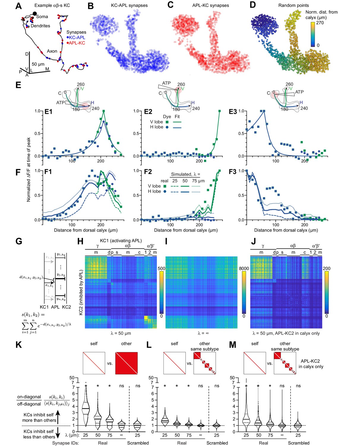
Localized activity and KC-APL anatomy suggest that KCs inhibit themselves more than other KCs.
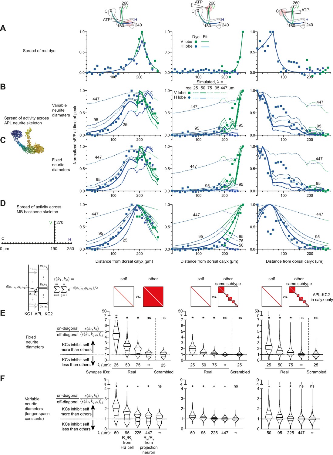
(A) Line drawing of an example αβs KC (body ID 5813078552). Soma shown by black circle (not to scale). KC-APL (blue circles) and APL-KC (red circles) synapses appear in the KC’s dendrites and axon. Dendritic KC-APL synapses are consistent with reports of presynaptic release from Kenyon cells in the calyx (Christiansen et al., 2011). Scale bar for (A–D), 50 µm, D, dorsal, V, vental, A, anterior, P, posterior, L, lateral, M, medial. (B,C) 2000 randomly selected synapses from the set of 96,867 unique KC-APL synapse locations (B) and 15,656 unique APL-KC synapse locations (C). The relative lack of KC-APL and APL-KC synapses in the posterior peduncle is consistent with the lack of syt-GFP signal in both APL and Kenyon cells in this zone, thought to be the Kenyon cells’ axon initial segment (Trunova et al., 2011; Wu et al., 2013). (D) 2000 random points along APL’s neurite skeleton, color-coded by normalized distance from the dorsal calyx along the average backbone skeleton in Figure 5. (E) Red dye signal from Figure 5 in 10 µm segments (dots), with fitted exponential decay curves (lines), for stimulation in the horizontal lobe (E1), vertical lobe (E2), and calyx (E3). The slight discontinuity in the curve fit for (E1) arises because the calyx-to-junction branch has slightly different fits for the calyx-to-vertical vs. calyx-to-horizontal branches; where the two merge, we averaged the fits together. (F) Real activity in APL from Figure 5 (dots) compared to simulated activity for different space constants (lines), given localized stimulation defined by fitted curves in (E) in the horizontal lobe (F1), vertical lobe (F2), and calyx (F3). (G) Schematic of metric s(k1,k2) for predicting how strongly KC1 inhibits KC2 via APL given the space constant λ and the relative distances (d) between KC1-APL (xi,k1) and APL-KC2 (yj,k2) synapses along APL’s neurite skeleton. The variable thickness of the APL-KC2 synapses depicts how synapses closer to the KC1-APL synapse (xi,k1) are weighted more strongly. The other KC1-APL synapses are greyed out to show that although they are part of the double summation, the focus in the diagram is on distances between xi,k1 and APL-KC2 synapses. (H) s(k1,k2) for all pairs of KCs, for space constant 50 µm. αβ, α′β′, γ subtypes as annotated in the hemibrain v1.1: γ subtypes: m, main; d, dorsal; γ-t subtype not labeled (t for thermo) – contains 8 KCs placed on the grid between (γ-m and γ-d). αβ: p, posterior; s, surface; c, core; m, intermediate KCs between surface and core. α′β′: 1, ap1; 2, ap2; m, medial, where ap corresponds to PAM-β′1ap and m corresponds to PAM-β′1 m (personal communication, S. Takemura). Note that s(k1,k2) is higher along the diagonal. KCs were sorted by subtype as annotated in the hemibrain dataset, and reordered by hierarchical clustering to place similar KCs within the same subtype next to each other. (I) As (H) except space constant is infinite. (J) As (H) except only including APL-KC synapses (yj,k2 in panel F) that are in the calyx. In (I–J), the order of KCs is preserved from (H). (K–M) The violin plots show, for each KC1, the ratio of s(k1,k1) (self-inhibition) vs. the average of s(k1,k2) across all k2 (inhibiting other KCs), given different space constants (λ), where k2 includes all other KCs (K), or all other KCs within the same subtype (L). Referring to (H–J), this ratio is each on-diagonal pixel divided by the average of the off-diagonal pixels in corresponding column. (M) As (L) except only including APL-KC synapses in the calyx. The squares above the violin plots mark in red which pixels are being analyzed from a heat map of s(k1,k2) as in panel H: that is, for ‘self’, the diagonal pixels; for ‘other’, the off-diagonal pixels; for ‘other, same subtype’, the off-diagonal pixels for KCs of the same subtype. ‘Synapse IDs’: For ‘Scrambled’ (but not ‘Real’), the identities of which Kenyon cell each KC-APL or APL-KC synapse belonged to were shuffled. Solid horizontal lines show the median; dotted lines show 25% and 75% percentile. n = 1923 KCs (4 of 1927 KCs annotated as KCγ-s1 through s4 – ‘s’ for ‘special’ – are excluded as there is only one example of each). *p<0.0001, different from 1.0 by Wilcoxon test with Holm-Bonferroni correction for multiple comparisons.
-
Figure 8—source data 1
Source data for Figure 8.
- https://cdn.elifesciences.org/articles/56954/elife-56954-fig8-data1-v2.xlsx
Figure 8—figure supplement 1
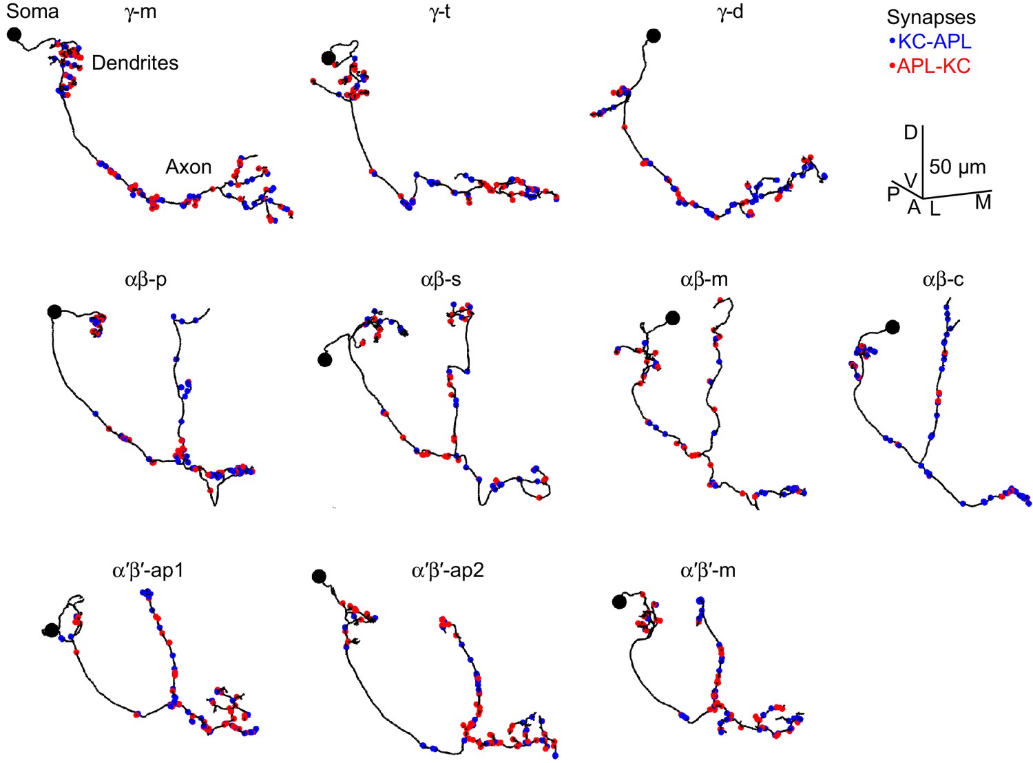
Example Kenyon cells.
Line drawings of example Kenyon cells of subtype γ-m (A), γ-t (B), γ-d (C), αβ-p (D), αβ-s (E), αβ-m (F), αβ-c (G), α′β′-ap1 (H), α′β′-ap2 (I), α′β′-m (J) from the hemibrain connectome (v1.1). γ-d and αβ-d Kenyon cells receive primarily visual input from the ventral and dorsal accessory calyces, respectively (Li et al., 2020; Vogt et al., 2016). The node with the biggest radius >1.25 µm was annotated as the soma (black circle); not all skeletons had a clear soma. Red circles, APL-KC synapses; blue circles, KC-APL synapses. Scale bar, 50 µm, D, dorsal, V, ventral, A, anterior, P, posterior, L, lateral, M, medial. bodyId numbers: (A) 5812981148, (B) 630731599, (C) 1004514714, (D) 456462835, (E) 5813055914, (F) 941111195, (G) 922677121, (H) 518864924, (I) 674393414, (J) 5812981553.
Figure 8—figure supplement 2
Additional data for Figure 8.
(A–D) Simulating local activation of APL with different space constants. Some curves have their space constants annotated for clarity (A) repeated from Figure 8E for comparison. (B) Simulated activity as in Figure 8F; simulated activity spreads farther than experimental activity spread when using longer space constants derived from published estimates of (λ = 95 µm derived from HS cells, or 447 µm derived from a projection neuron). (C) As in B but treating all APL neurites as having the same diameter (see Materials and methods). Simulated activity spreads somewhat further than in B, likely because the very thin APL neurites are likely ‘branches’ rather than ‘main trunk’ neurites along which signals would have to travel to go across the neuron. (D) Simulated activity ignoring APL neurite morphology, treating the Voronoi cells as points on perpendicular straight lines. The same exponential decay applies as in B, except that the distance between points is the cityblock distance, that is, the distance along the backbone skeleton, not the APL’s neurite skeleton (as in B–C): . Note that 50 µm gives the best fit for horizontal lobe and calyx stimulation, while 25 µm gives the best fit for vertical lobe stimulation. (E) As Figure 8K–M, except treating all APL neurites as having the same diameter. (F) As Figure 8K–M, except including longer space constants (50 µm and infinity repeated for comparison). Significant imbalance in self vs. other inhibition remains even at λ = 95 and 225 µm.
-
Figure 8—figure supplement 2—source data 1
Source data for Figure 8—figure supplement 2.
- https://cdn.elifesciences.org/articles/56954/elife-56954-fig8-figsupp2-data1-v2.xlsx
Figure 8—figure supplement 3
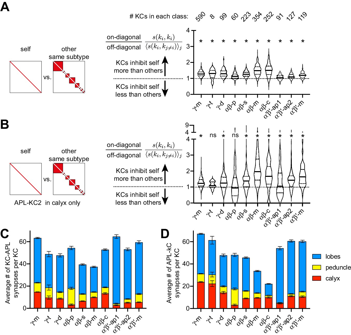
Self- vs. other-inhibition in different Kenyon cell subtypes.
(A) As Figure 8K but separating out different Kenyon cell subtypes as annotated in the hemibrain v. 1.1 (λ = 50 µm). (B) As (A) but only including APL-KC synapses in the calyx. *p<0.05, different from 1.0 by Wilcoxon test with Holm-Bonferroni correction for multiple comparisons. The lack of significant imbalance in γ-t Kenyon cells is likely because there are only eight such Kenyon cells. (C–D) Average number of KC-APL (C) and APL-KC (D) synapses per KC in the calyx (red), peduncle (yellow) or lobes (blue). Note that αβ-p Kenyon cells, the only substantial subtype with no significant imbalance in (B), form few synapses with APL in the calyx. Error bars, 95% confidence interval.
-
Figure 8—figure supplement 3—source data 1
Source data for Figure 8—figure supplement 3.
- https://cdn.elifesciences.org/articles/56954/elife-56954-fig8-figsupp3-data1-v2.xlsx
Figure 8—figure supplement 4
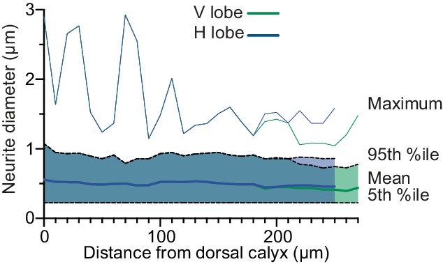
Diameter of APL neurites.
Line shows mean neurite diameter in each Voronoi cell of APL, shaded area shows 5th to 95th percentile, and thin line above shows the maximum. Mean and percentiles were calculated by weighting each link in APL’s neurite skeleton by its length. Distance from calyx measured along the backbone skeleton (Figure 5).
Appendix 1—figure 1
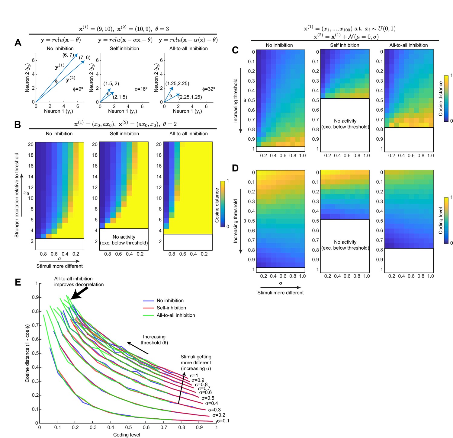
All-to-all inhibition decorrelates population activity better than self-inhibition.
(A) For a toy example of two neurons and two stimuli, self-inhibition improves the stimulus separation (i.e, increases angle between the two stimulus vectors) by bringing activity down closer to spiking threshold, but all-to-all inhibition improves the separation more. Note that to simplify the model, we model the inhibitory interneuron as being activated by the principal neurons' dendrites, as occurs with Kenyon cells and APL. (B) Generalization of result in (A) to wider activity range in the two neurons. Heat maps show cosine distance for different values of and a (increasing means more excitation; decreasing a means the stimuli are more different). The self-inhibition panel is the same as the no-inhibition panel, just stretched vertically (i.e., self-inhibition acts as gain control), whereas the all-to-all inhibition panel expands the range of high cosine distances toward more similar stimulus pairs. Blank areas mean the activity is zero because excitation is below threshold, so cosine distance is undefined. (C) Generalization of (A,B) to population of 100 neurons. Stimulus 1 is sampled from a uniform distribution over (0, 1). Stimulus 2 is Stimulus 1 plus Gaussian noise (magnitude of noise governed by σ; higher σ means the two stimuli are more different). Heat maps show cosine distance for different thresholds (θ) and σ averaged over 100 trials. (D) Coding level (fraction of active neurons) for different thresholds and σ as in (C); note how decreasing coding level (increased sparseness) correlates with higher cosine distance. (E) Each curve is one column (one value of σ) from the heat maps in (C) and (D), showing how cosine distance improves with lower coding levels. Adding inhibition does not change this curve; it merely shifts the model to different points along the curve. All-to-all inhibition achieves higher cosine distance (more decorrelated activity) than self-inhibition or no inhibition.
Tables
Key resources table
| Reagent type (species) or resource | Designation | Source or reference | Identifiers | Additional information |
|---|---|---|---|---|
| Genetic reagent (D. melanogaster) | OK107-GAL4 | Connolly et al., 1996 | BDSC:854 | |
| Genetic reagent (D. melanogaster) | MB247-DsRed | Riemensperger et al., 2005, | FLYB:FBtp0022384 | |
| Genetic reagent (D. melanogaster) | UAS-GCaMP6f (VK00005) | Chen et al., 2013, | BDSC:52869 FLYB: FBst0052869 | |
| Genetic reagent (D. melanogaster) | UAS-GCaMP6f (attP40) | Chen et al., 2013, | BDSC:42747 FLYB: FBst0042747 | |
| Genetic reagent (D. melanogaster) | tub-FRT-GAL80-FRT | Gordon and Scott, 2009; Lin et al., 2014 | BDSC:38880 | |
| Genetic reagent (D. melanogaster) | MB247-LexA | Lin et al., 2014; Pitman et al., 2011 | FLYB:FBtp0070099 | |
| Genetic reagent (D. melanogaster) | LexAop-P2X2 | This study | See ‘Fly strains and husbandry’ | |
| Genetic reagent (D. melanogaster) | LexAop-GCaMP6f | Barnstedt et al., 2016 | Gift from S. Waddell | |
| Genetic reagent (D. melanogaster) | GH146-FLP | Hong et al., 2009, | FLYB:FBtp0053491 | |
| Genetic reagent (D. melanogaster) | UAS-mCherry-CAAX | Kakihara et al., 2008; Lin et al., 2014 | FLYB:FBtp0041366 | |
| Genetic reagent (D. melanogaster) | NP2631-GAL4 | Tanaka et al., 2008 | DGRC:104266 | |
| Genetic reagent (D. melanogaster) | UAS-P2X2 | Lima and Miesenböck, 2005 | BDSC:76032 FLYB: FBtp0021869 | |
| Genetic reagent (D. melanogaster) | UAS-P2X2 (attP40) | Clowney et al., 2015 | Gift from V. Ruta | |
| Genetic reagent (D. melanogaster) | VT43924-GAL4.2 | This study | See ‘Fly strains and husbandry’ | |
| Genetic reagent (D. melanogaster) | UAS-CD8::GFP | Lee et al., 1999 | BDSC:5130 FLYB: FBst0005130 | |
| Genetic reagent (D. melanogaster) | 474-GAL4 | Silies et al., 2013 | BDSC:63344 FLYB: FBst0063344 | |
| Genetic reagent (D. melanogaster) | 853-GAL4 | Silies et al., 2013 {Gao:2015fk} | InSITE database 0853 | |
| Genetic reagent (D. melanogaster) | mb247-GAL4 | Zars et al., 2000 | ||
| Genetic reagent (D. melanogaster) | c739-GAL4 | Yang et al., 1995, | BDSC:7362 FLYB: FBst0007362 | |
| Genetic reagent (D. melanogaster) | NP3061-GAL4 | Tanaka et al., 2008, | DGRC:104360 FLYB:FBti0035130 | |
| Genetic reagent (D. melanogaster) | QUAS-GCaMP3 | This study | See ‘Fly strains and husbandry’ | |
| Genetic reagent (D. melanogaster) | GH146-QF | Potter et al., 2010 | BDSC:30015 FLYB: FBti0129854 | |
| Genetic reagent (D. melanogaster) | UAS-Ort | Liu and Wilson, 2013 | Gift from Chi-hon Lee |
Additional files
-
Supplementary file 1
List of full genotypes.
- https://cdn.elifesciences.org/articles/56954/elife-56954-supp1-v2.docx
-
Supplementary file 2
Details of statistical analysis.
- https://cdn.elifesciences.org/articles/56954/elife-56954-supp2-v2.xlsx
-
Transparent reporting form
- https://cdn.elifesciences.org/articles/56954/elife-56954-transrepform-v2.docx
Download links
A two-part list of links to download the article, or parts of the article, in various formats.
Downloads (link to download the article as PDF)
Open citations (links to open the citations from this article in various online reference manager services)
Cite this article (links to download the citations from this article in formats compatible with various reference manager tools)
Localized inhibition in the Drosophila mushroom body
eLife 9:e56954.
https://doi.org/10.7554/eLife.56954


