Improving a probabilistic cytoarchitectonic atlas of auditory cortex using a novel method for inter-individual alignment
- Department of Cognitive Neuroscience, Maastricht University, Netherlands
- Brain Innovation B.V, Netherlands
- Maastricht Centre for Systems Biology, Faculty of Science and Engineering, Maastricht University, Netherlands
- Institute for Neuroscience and Medicine (INM-1), and JARA Brain, Research Centre Jülich, Germany
- C. and O. Vogt Institute for Brain Research, Heinrich Heine University, Germany
- Center for Magnetic Resonance Research, University of Minnesota, United States
Figures
Figure 1

Differences between spherical rigid body alignment, curvature-based alignment (CBA), and CBA with an anatomical prior (CBA+) on group average binarized curvature maps visualized as half-sphere projections (rows 1 and 3) and group average vertex coordinates visualized as folded surfaces (rows 2 and 4).
In rows 1 and 3, higher contrast between sulci (dark gray) and gyri (light gray) shows more overlap around Heschl’s Gyrus which indicates that a method better accounts for inter-subject morphological variation. In rows 2 and 4, the average vertex coordinates show a more pronounced Heschl’s Gyrus in 3D as the alignment method improves the anterior Heschl’s Gyrus overlap.
Figure 2
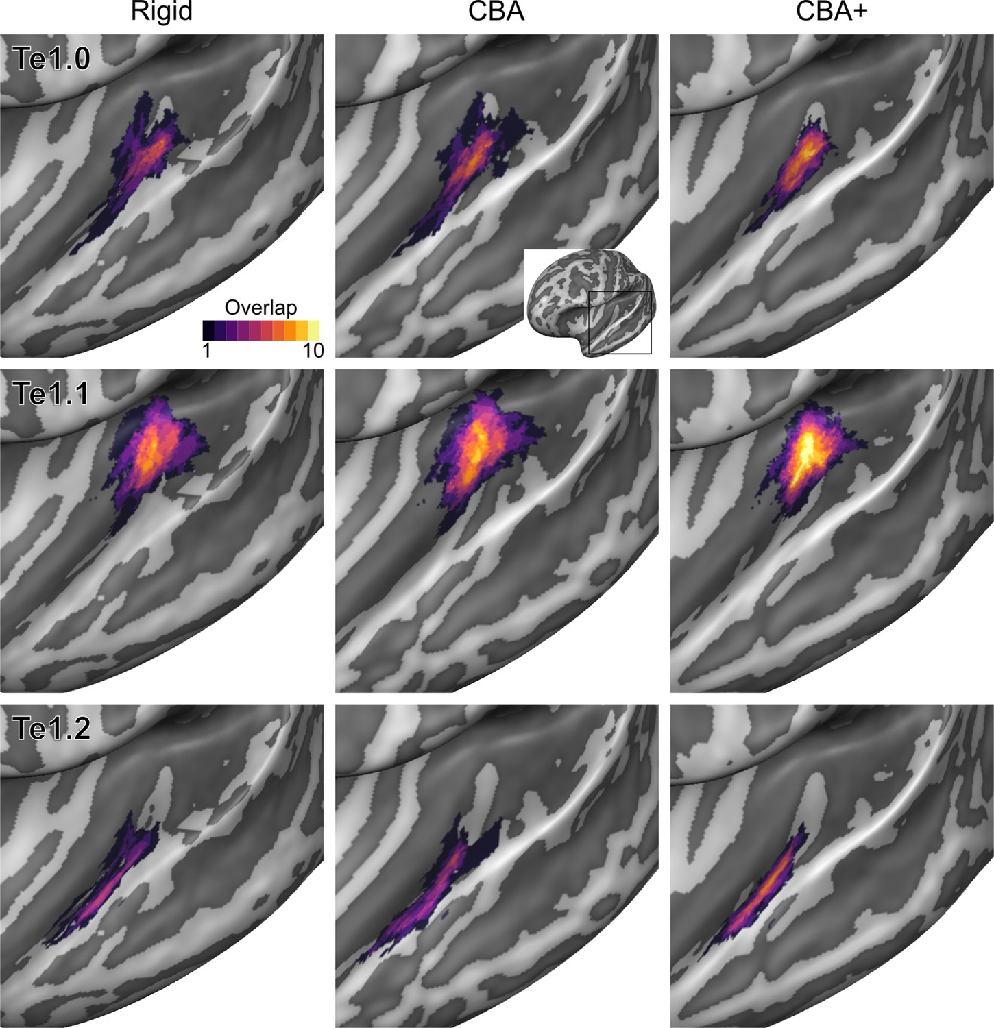
Probabilistic maps (after alignment) indicating the number of subjects for which a given vertex is labeled as belonging to the cytoarchitectonic areas Te1.0, Te1.1 and Te1.2 are presented on inflated group average cortical surfaces of the left hemisphere.
Columns show spherical rigid body alignment, curvature-based alignment (CBA) and CBA with anatomical priors (CBA+) from left to right. Improvements in the micro-anatomical correspondence diminishes low values in the maps (purple) and increases the presence of high probability values (yellow).
Figure 3
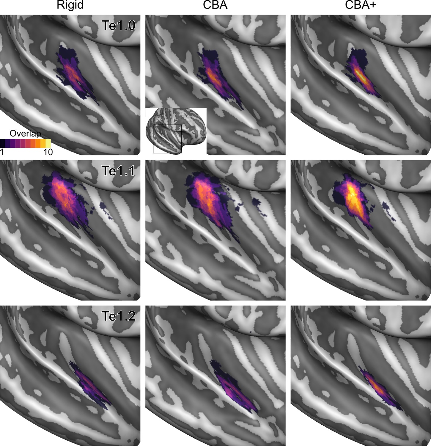
Probabilistic maps (after alignment) indicating the number of subjects for which a given vertex is labeled as belonging to the cytoarchitectonic areas Te1.0, Te1.1 and Te1.2 are presented on inflated group average cortical surfaces of the right hemisphere.
Columns show spherical rigid body alignment, curvature-based alignment (CBA) and CBA with anatomical priors (CBA+) from left to right. Improvements in the micro-anatomical correspondence diminishes low values in the maps (purple) and increases the presence of high probability values (yellow).
Figure 4
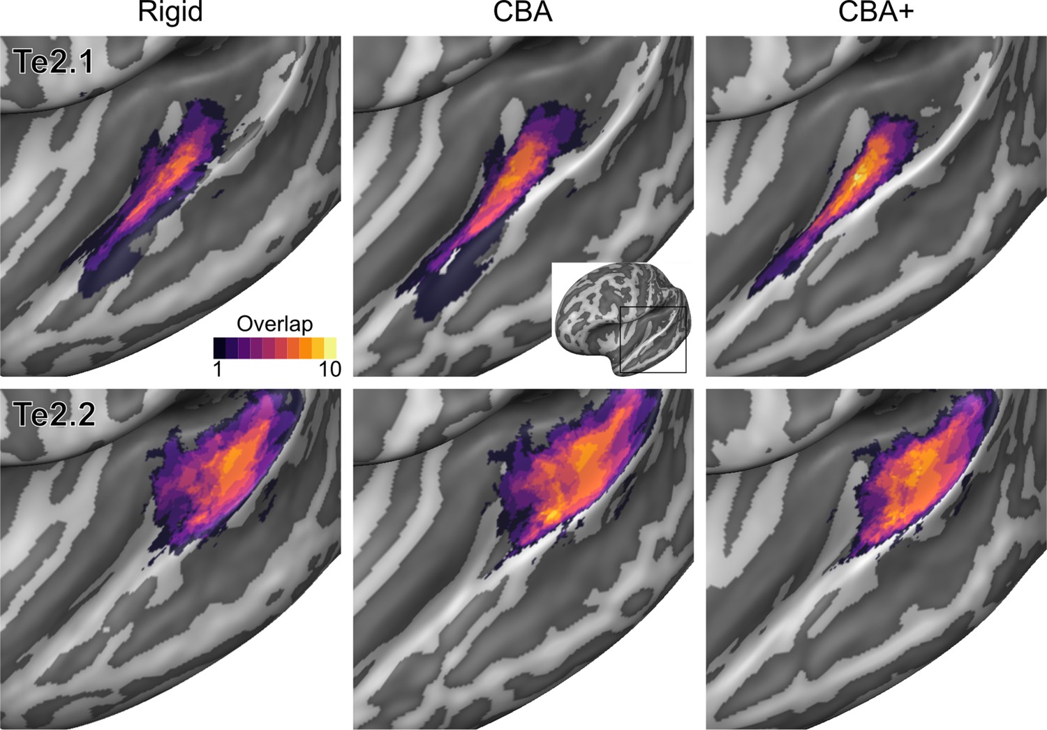
Probabilistic maps (after alignment) indicating the number of subjects for which a given vertex is labeled as belonging to the cytoarchitectonic areas Te2.1 and Te2.2 are presented on inflated group average cortical surfaces of the left hemisphere.
Columns show spherical rigid body alignment, curvature-based alignment (CBA) and CBA with anatomical priors (CBA+) from left to right. Improvements the micro-anatomical correspondence diminishes low values in the maps (purple) and increases the presence of high probability values (yellow).
Figure 5
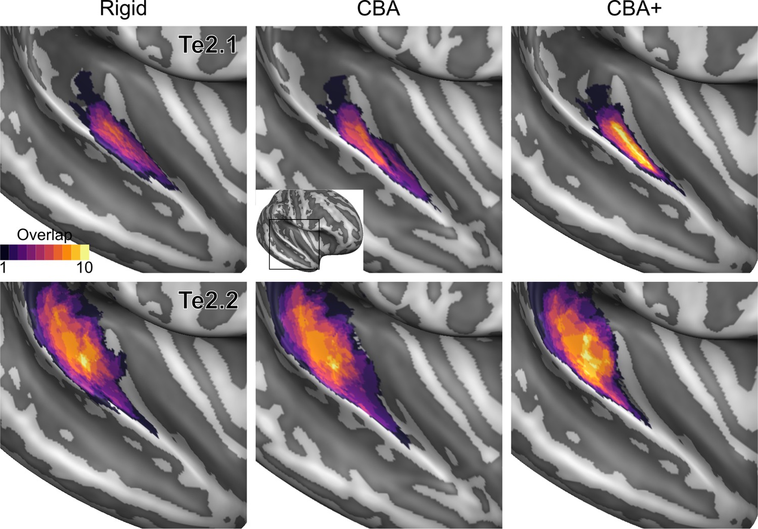
Probabilistic maps (after alignment) indicating the number of subjects for which a given vertex is labeled as belonging to the cytoarchitectonic areas Te2.1 and Te2.2 are presented on inflated group average cortical surfaces of the right hemisphere.
Columns show spherical rigid body alignment, curvature-based alignment (CBA) and CBA with anatomical priors (CBA+) from left to right. Improvements in the micro-anatomical correspondence diminishes low values in the maps (purple) and increases the presence of high probability values (yellow).
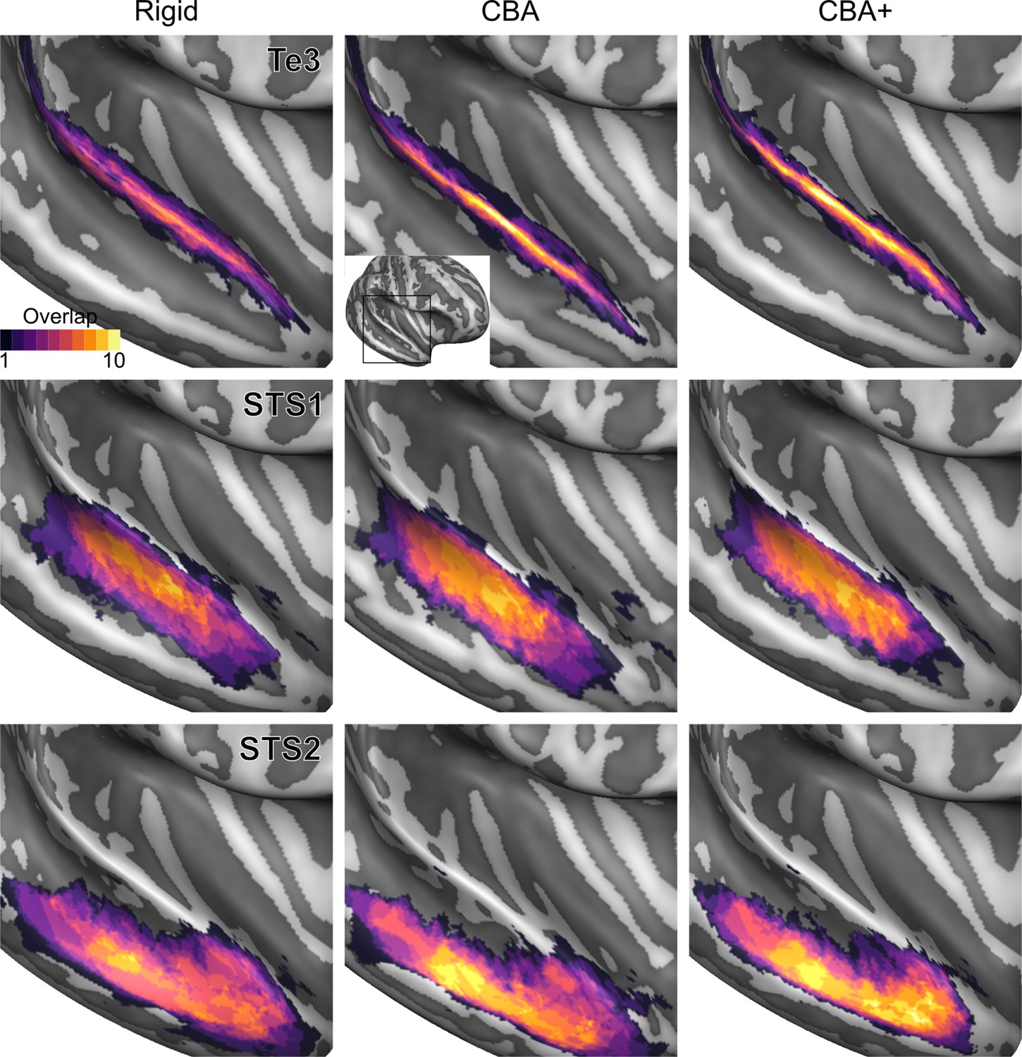
Figure 6

Probabilistic maps (after alignment) indicating the number of subjects for which a given vertex is labeled as belonging to the cytoarchitectonic areas Te3, STS1 and STS2 are presented on inflated group average cortical surfaces of the left hemisphere.
Columns show spherical rigid body alignment, curvature-based alignment (CBA) and CBA with anatomical priors (CBA+) from left to right. Improvements in the micro-anatomical correspondence diminishes low values in the maps (purple) and increases the presence of high probability values (yellow).
Figure 7
Probabilistic maps (after alignment) indicating the number of subjects for which a given vertex is labeled as belonging to the cytoarchitectonic areas Te3, STS1 and STS2 are presented on inflated group average cortical surfaces of the right hemisphere.
Columns show spherical rigid body alignment, curvature-based alignment (CBA) and CBA with anatomical priors (CBA+) from left to right. Improvements in the micro-anatomical correspondence diminishes low values in the maps (purple) and increases the presence of high probability values (yellow).
Figure 8
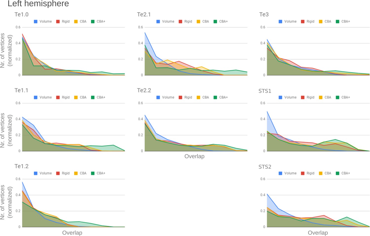
Histograms of the overlap across cytoarchitectonic areas in the left hemisphere.
The histograms are normalized by the number of vertices per area. The x-axis represents the probability value (an overlap from 1 out of ten [left] to 10 out of 10 participants [right]). The ideal co-registration method should show a less left skewed distribution. CBA+ shows the lowest skew towards the left in comparison to other methods.
Figure 9
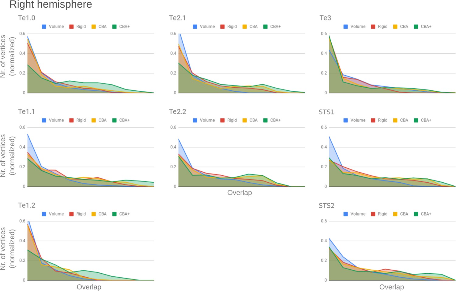
Histograms of the overlap across cytoarchitectonic areas in the right hemisphere.
The histograms are normalized by the number of vertices per area. The x-axis represents the probability value (an overlap from 1 out of 10 [left] to 10 out of 10 participants [right]). The ideal co-registration method should show less left skewed distribution. CBA+ shows the lowest skew toward the left in comparison to other methods.
Figure 10 with 11 supplements

Relation between group average (CBA+) in vivo MRI measures and the cytoarchitectonic atlas.
The cytoarchitectonic areas are delineated with black lines. The myelination index is computed from the division of T1w and T2*w data. Tonotopy reflects the voxel-wise frequency preference estimated with fMRI encoding from the response to natural sound stimuli. All measures are sampled on the middle gray matter surfaces.
Figure 10—figure supplement 1
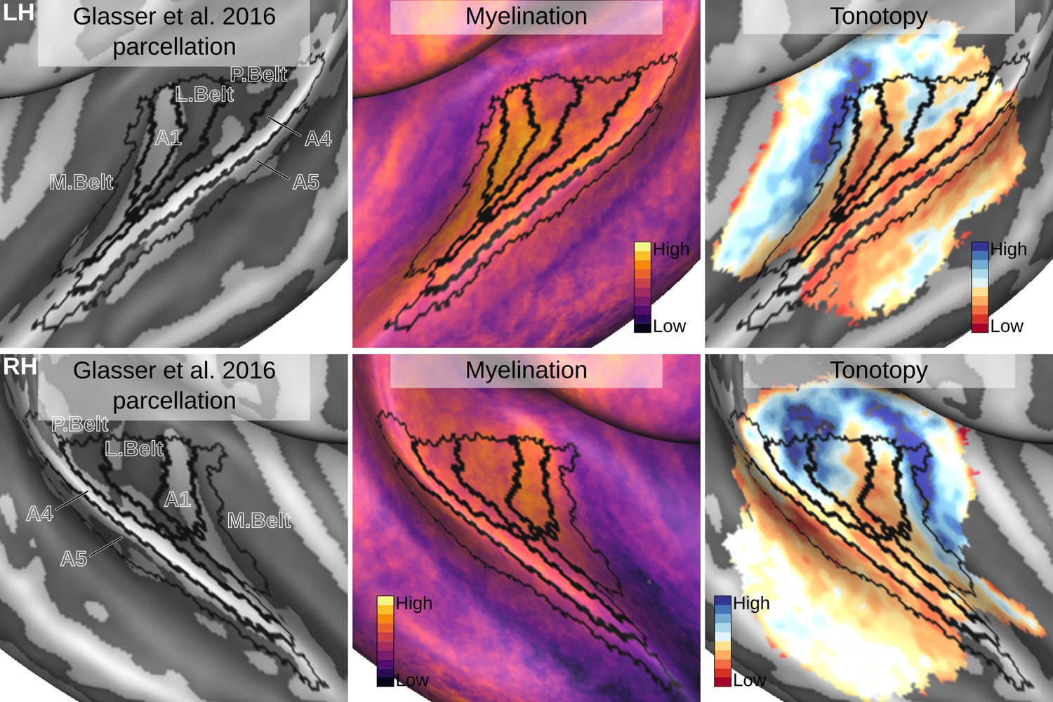
The same maps projected on an in vivo multi-modal MRI group atlas (Glasser et al., 2016).
Relation between the in vivo MRI measures of the left hemisphere and the multi-modal MRI-based parcellation. The multi-modal MRI-based parcellation from Glasser et al., 2016 is delineated with black lines. The myelination index is computed from the division of T1w and T2*w data. Tonotopy reflects the voxel-wise frequency preference estimated with fMRI encoding from the response to natural sound stimuli. All measures are sampled on the middle gray matter surfaces.
Figure 10—figure supplement 2
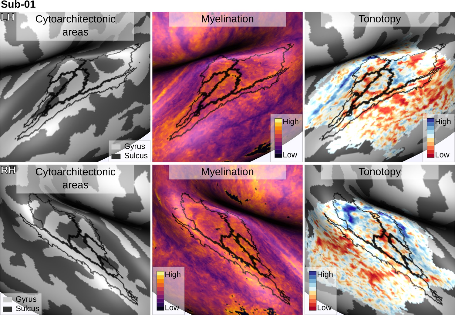
Individual brain in vivo MRI measures of Subject 01.
Subject 01, relation between in vivo MRI measures and the cytoarchitectonic atlas.
Figure 10—figure supplement 3
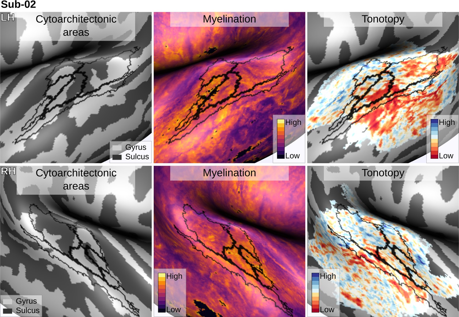
Individual brain in vivo MRI measures of Subject 02.
Subject 02, relation between in vivo MRI measures and the cytoarchitectonic atlas.
Figure 10—figure supplement 4

Individual brain in vivo MRI measures of Subject 03.
Subject 03, relation between in vivo MRI measures and the cytoarchitectonic atlas.
Figure 10—figure supplement 5
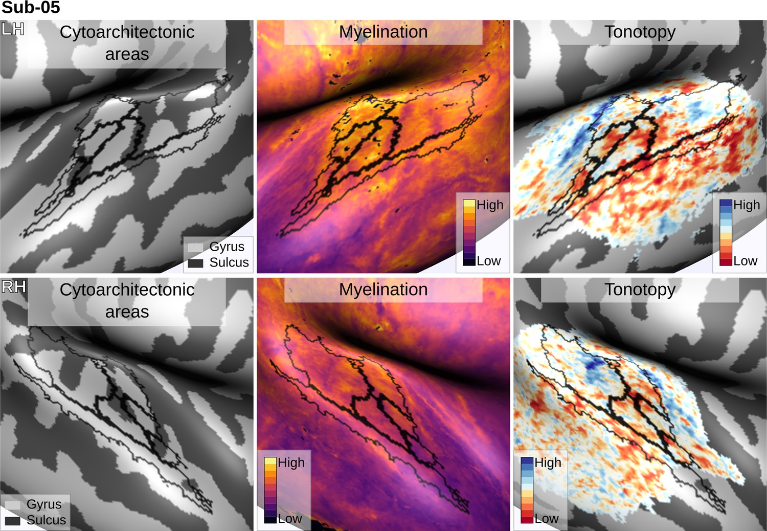
Individual brain in vivo MRI measures of Subject 05.
Subject 05, relation between in vivo MRI measures and the cytoarchitectonic atlas.
Figure 10—figure supplement 6
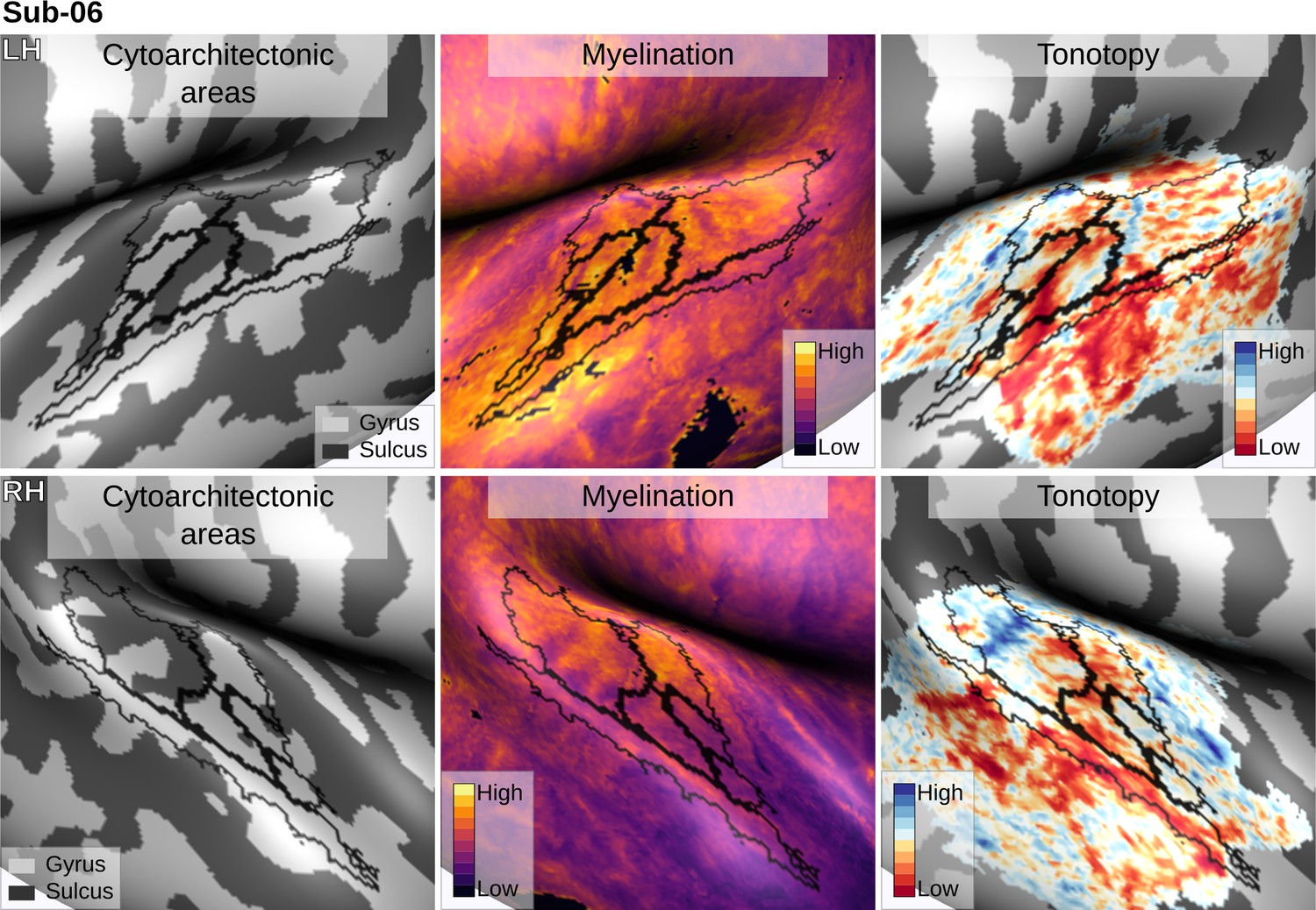
Individual brain in vivo MRI measures of Subject 06.
Subject 06, relation between in vivo MRI measures and the cytoarchitectonic atlas.
Figure 10—figure supplement 7
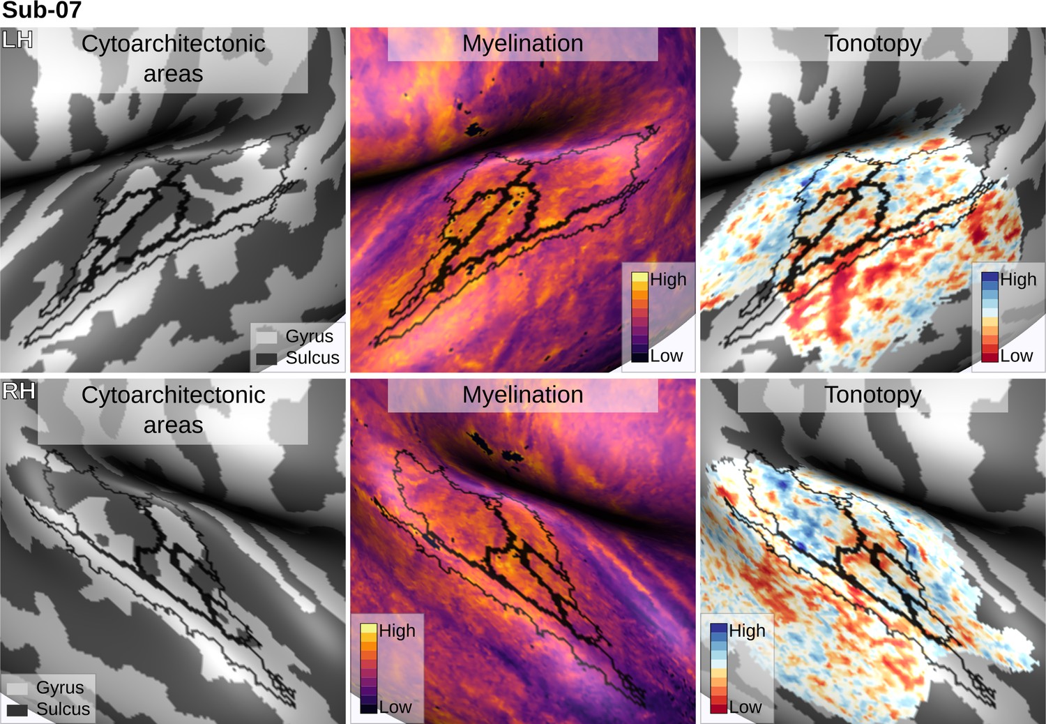
Individual brain in vivo MRI measures of Subject 07.
Subject 07, relation between in vivo MRI measures and the cytoarchitectonic atlas.
Figure 10—figure supplement 8
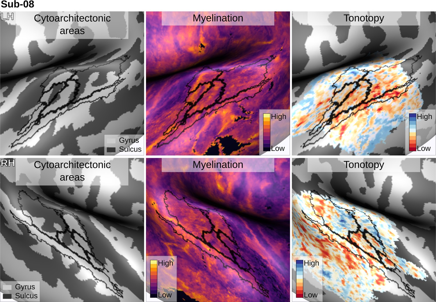
Individual brain in vivo MRI measures of Subject 08.
Subject 08, relation between in vivo MRI measures and the cytoarchitectonic atlas.
Figure 10—figure supplement 9
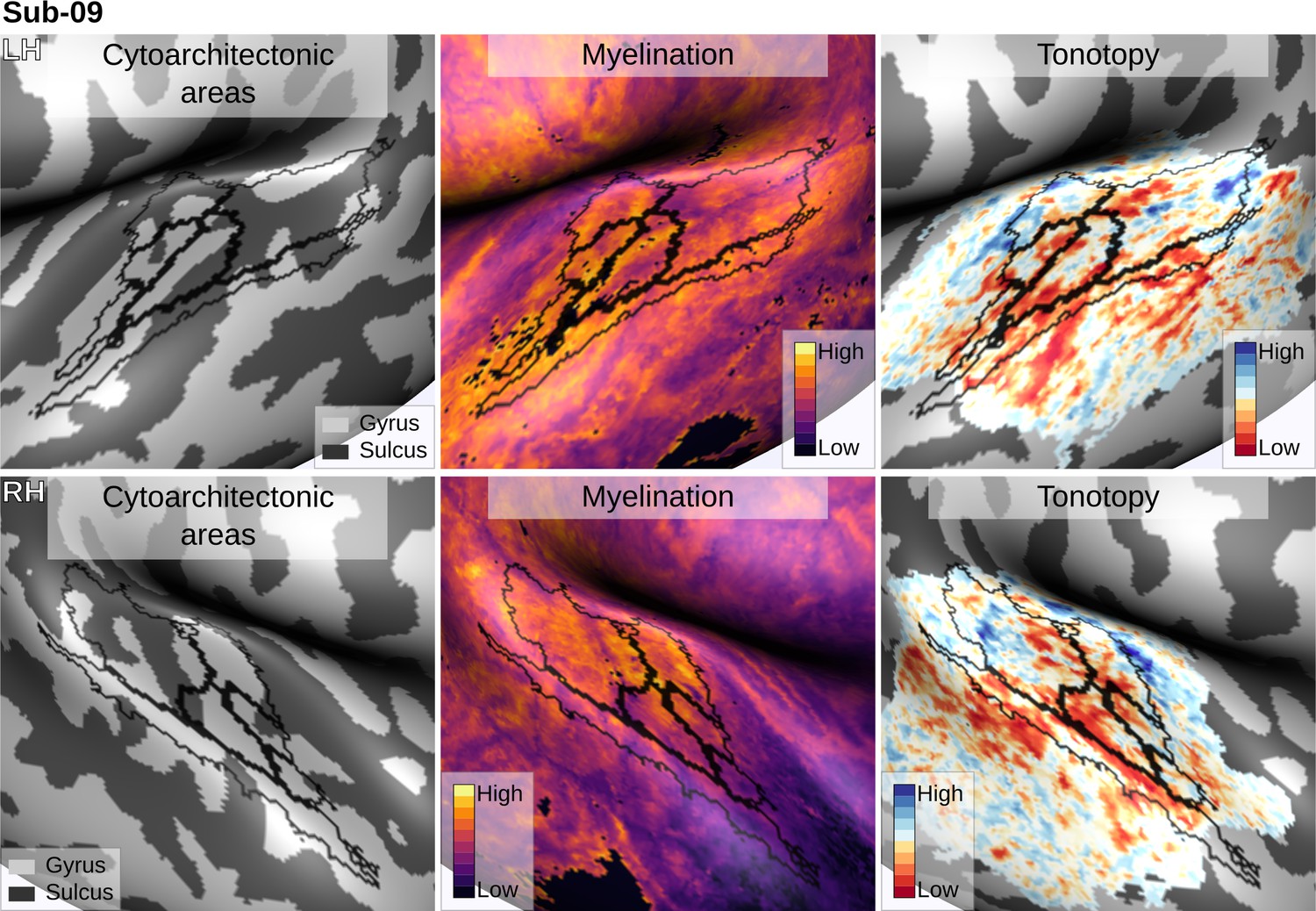
Individual brain in vivo MRI measures of Subject 09.
Subject 09, relation between in vivo MRI measures and the cytoarchitectonic atlas.
Figure 10—figure supplement 10
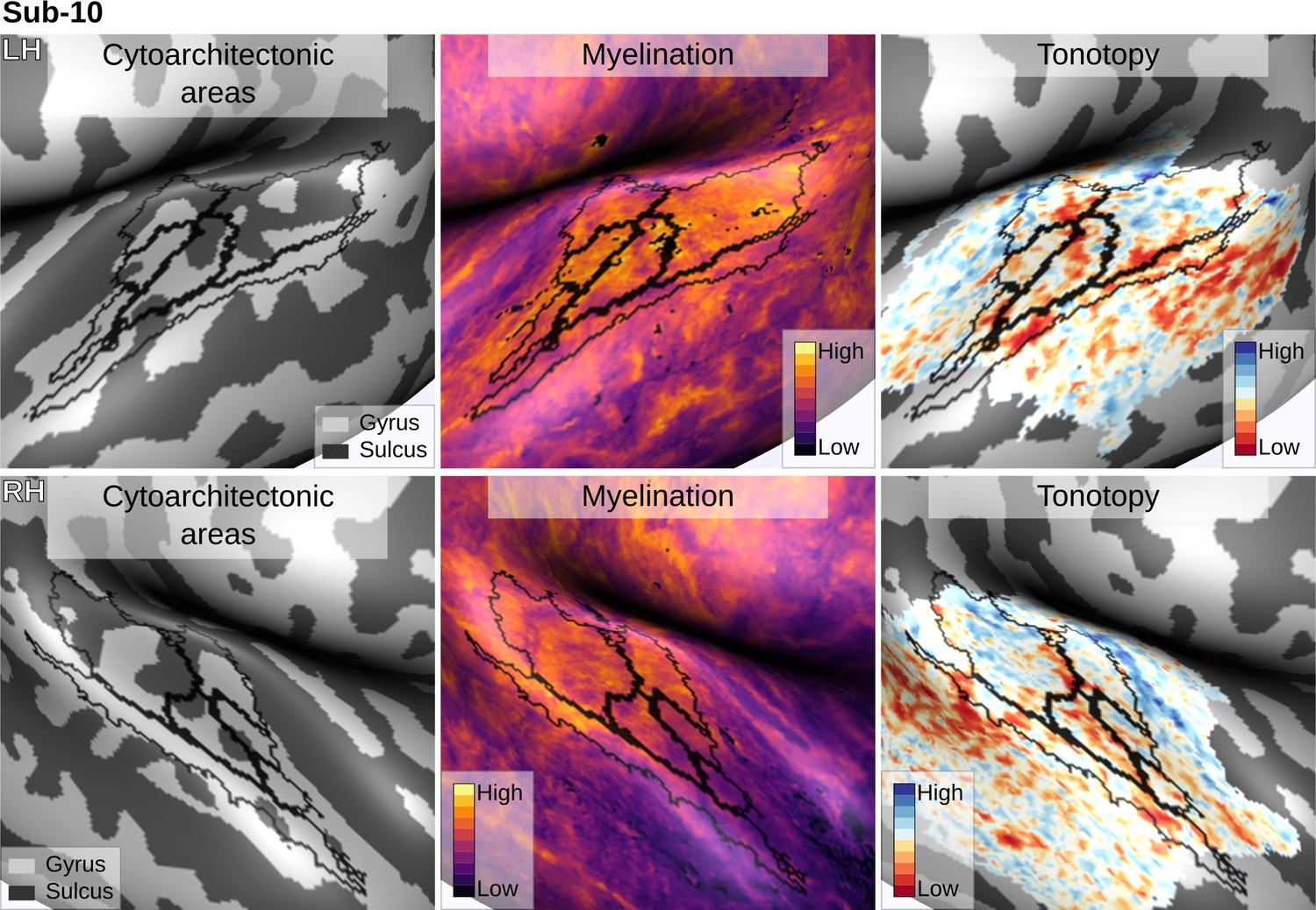
Individual brain in vivo MRI measures of Subject 10.
Subject 10, relation between in vivo MRI measures and the cytoarchitectonic atlas.
Figure 10—figure supplement 11
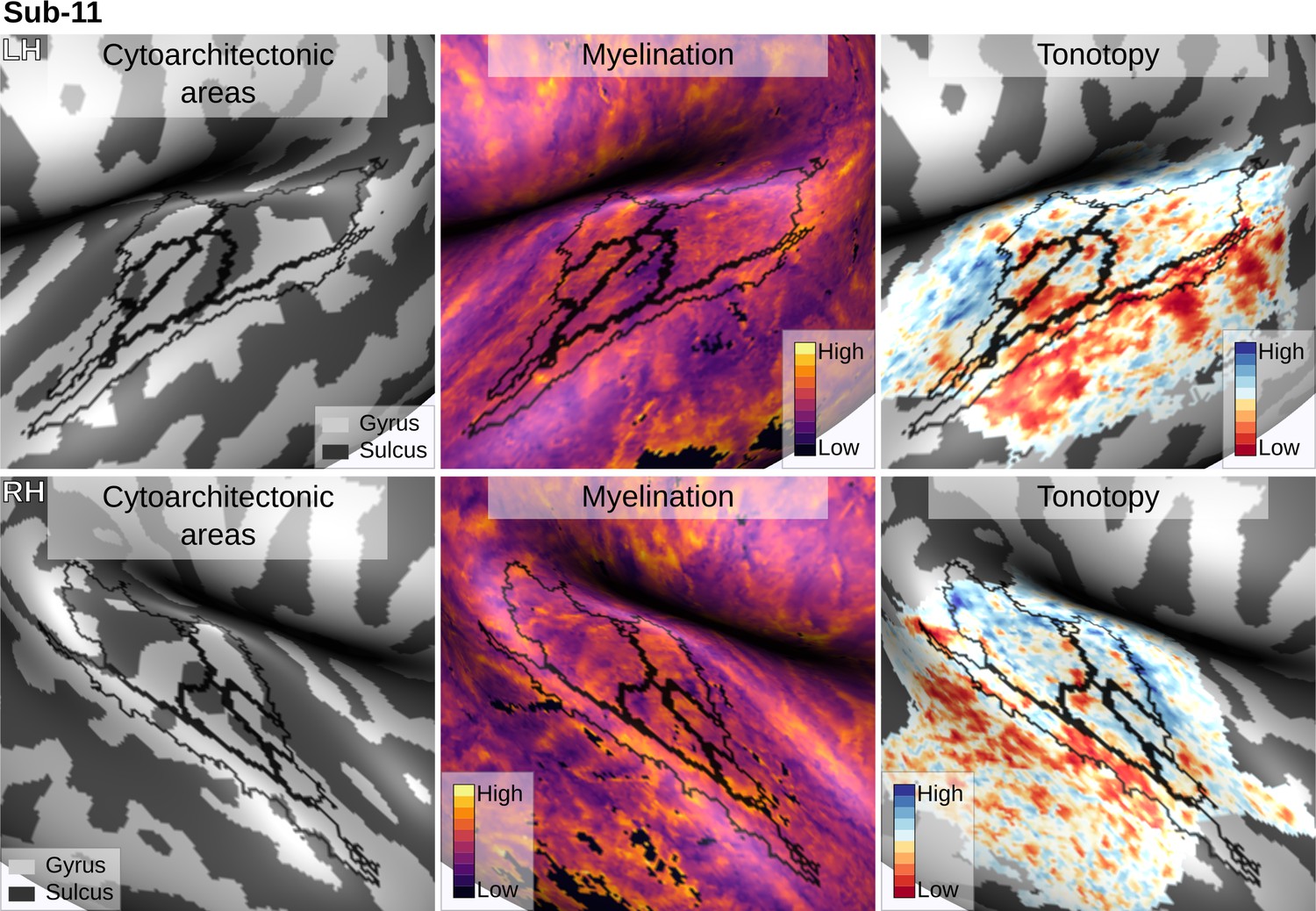
Individual brain in vivo MRI measures of Subject 11.
Subject 11, relation between in vivo MRI measures and the cytoarchitectonic atlas.
Figure 11

Comparison of cytoarchitectonic areas Morosan et al., 2001; Morosan et al., 2005 and multi-modal MRI-based labels (Glasser et al., 2016).
Areas on Heschl’s Gyrus differ between the two atlases.
Figure 12
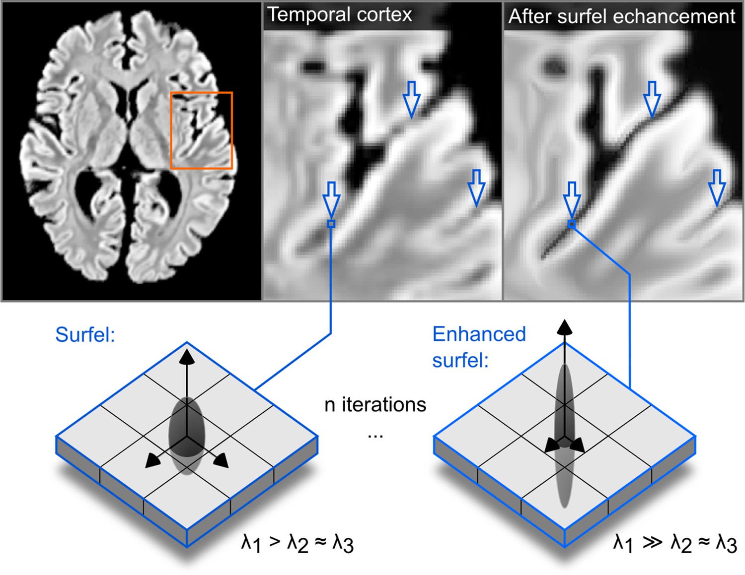
The effect of the structure enhancing filter shown on a transversal slice.
Blue arrows point to locations where local contrast is sharpened.
Figure 13
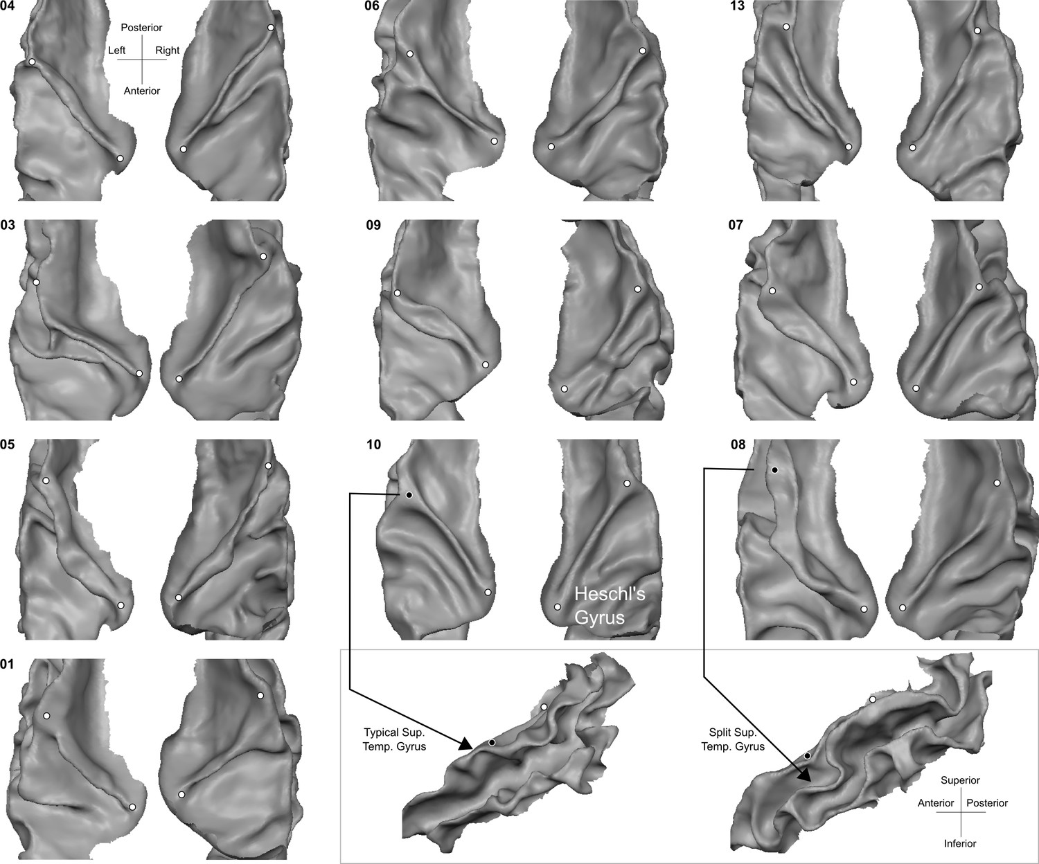
Individual superior temporal cortex white-gray matter boundary reconstructions.
Anterior Heschl’s Gyrus is indicated as the gyrus between white dots. The bottom right side shows the rare occurrence of a split superior temporal gyrus (Heschl, 1878) in contrast to a typical superior temporal gyrus from the side view.
Figure 14
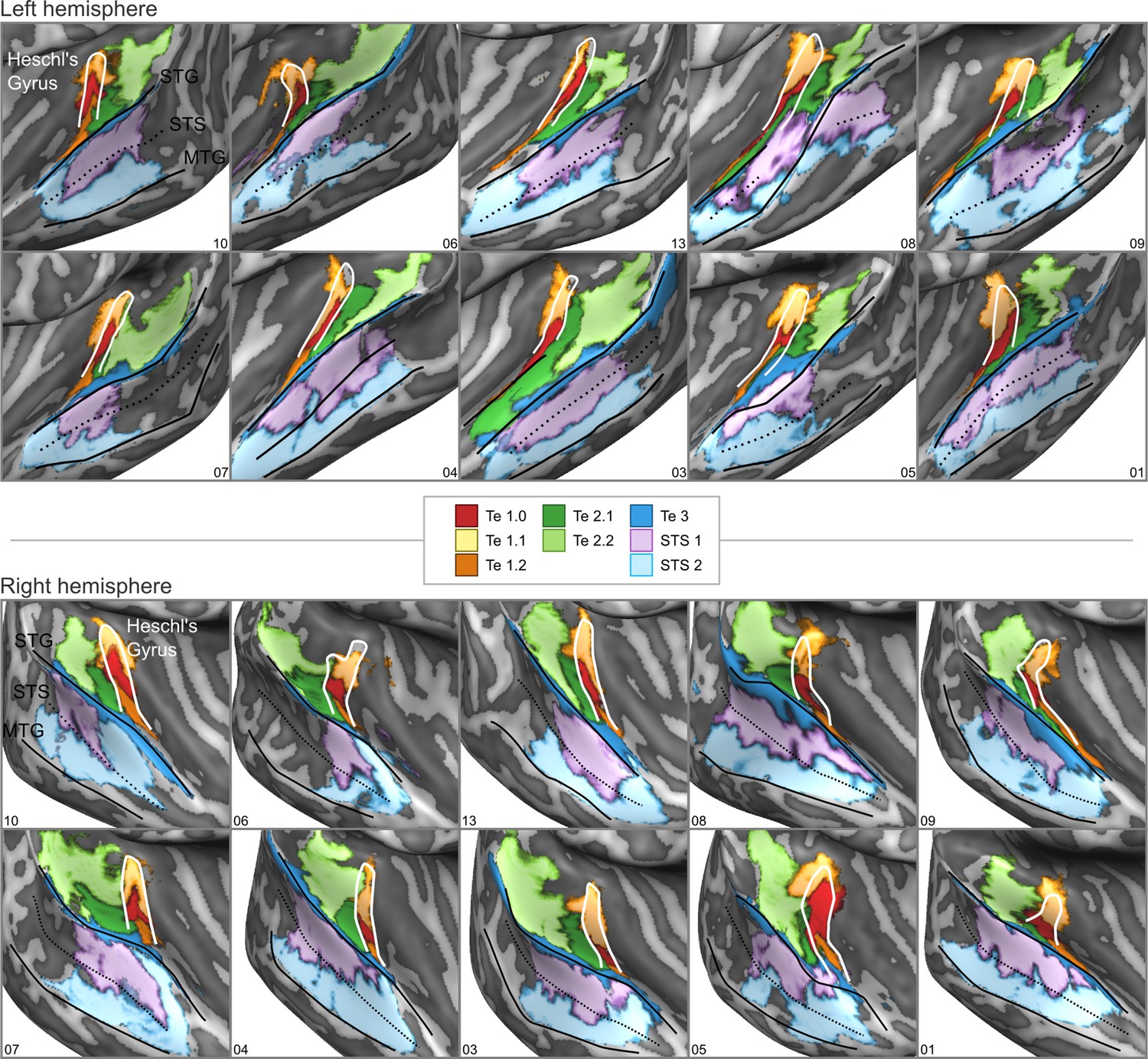
cytoarchitectonic areas of Morosan et al., 2001; Morosan et al., 2005; Zachlod et al., 2020 sampled on the inflated cortical surfaces for each individual brain in the postmortem dataset.
Anterior Heschl’s Gyrus, superior temporal gyrus (STG), superior temporal sulcus (STS), and middle temporal gyrus (MTG) are indicated as line drawings.
Figure 15
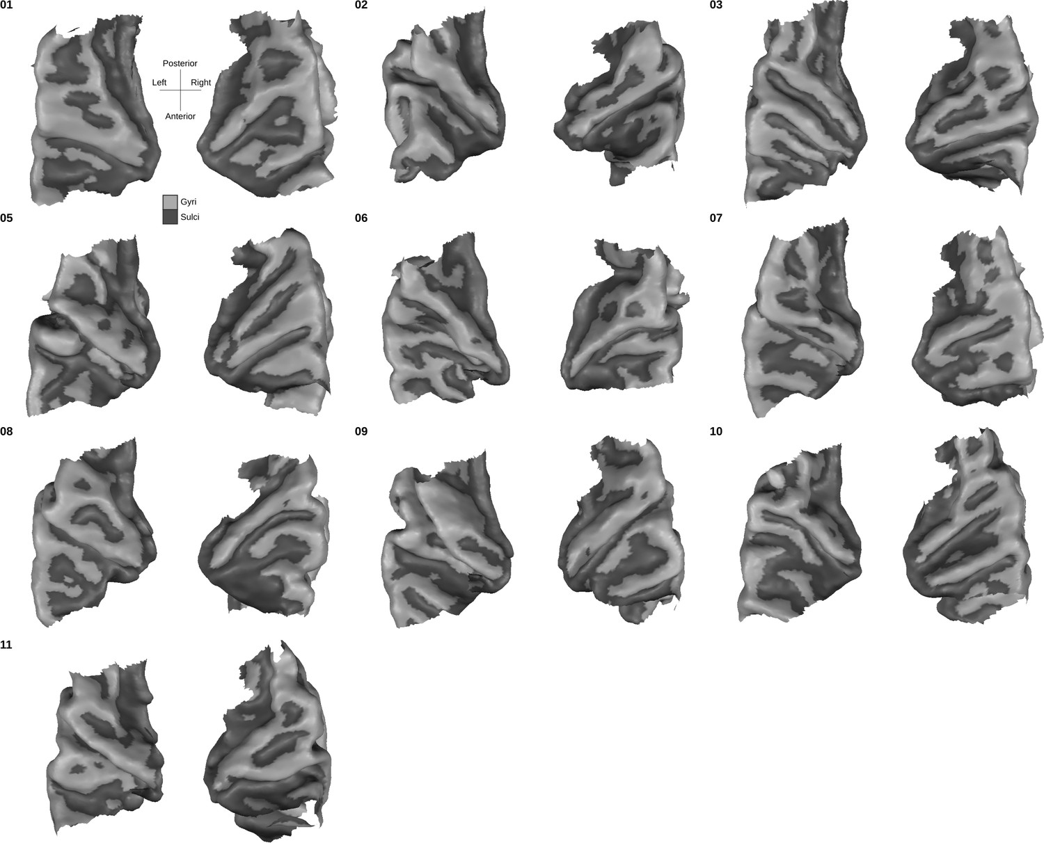
Individual superior temporal cortex middle-gray matter surface reconstructions from a bird’s eye (top-down) view.
Dark gray colored indicate sulci and light gray indicates gyri.
Tables
Table 1
DICE coefficients computed for each area using a leave-one-subject out approach for the areas in left hemispheres.
Using rigid body alignment, CBA, or CBA+, the surface area of each area from the left-out subject is compared to an atlas obtained from the remaining nine subjects. The atlas in this case is constructed by considering the vertices that overlap in at least four out of the nine subjects.
| RIGID | ||||||||||||
|---|---|---|---|---|---|---|---|---|---|---|---|---|
| Area | Sub-01 | Sub-03 | Sub-04 | Sub-05 | Sub-06 | Sub-07 | Sub-08 | Sub-09 | Sub-10 | Sub-13 | Mean | Std. Dev. |
| Te 1.0 | 0.23 | 0.47 | 0.42 | 0.36 | 0.40 | 0.00 | 0.43 | 0.45 | 0.02 | 0.12 | 0.29 | 0.18 |
| Te 1.1 | 0.50 | 0.71 | 0.54 | 0.62 | 0.62 | 0.09 | 0.67 | 0.49 | 0.33 | 0.15 | 0.47 | 0.21 |
| Te 1.2 | 0.03 | 0.40 | 0.02 | 0.25 | 0.43 | 0.00 | 0.00 | 0.18 | 0.23 | 0.00 | 0.15 | 0.17 |
| Te 2.1 | 0.56 | 0.42 | 0.43 | 0.49 | 0.70 | 0.00 | 0.34 | 0.40 | 0.22 | 0.22 | 0.38 | 0.20 |
| Te 2.2 | 0.36 | 0.49 | 0.57 | 0.64 | 0.57 | 0.49 | 0.62 | 0.55 | 0.10 | 0.09 | 0.45 | 0.20 |
| Te 3 | 0.26 | 0.11 | 0.08 | 0.23 | 0.35 | 0.01 | 0.20 | 0.35 | 0.15 | 0.27 | 0.20 | 0.11 |
| Te 4 | 0.57 | 0.41 | 0.61 | 0.54 | 0.64 | 0.27 | 0.34 | 0.40 | 0.70 | 0.64 | 0.51 | 0.15 |
| Te 5 | 0.54 | 0.41 | 0.65 | 0.45 | 0.69 | 0.43 | 0.29 | 0.57 | 0.61 | 0.54 | 0.52 | 0.12 |
| CBA | ||||||||||||
| Area | Sub-01 | Sub-03 | Sub-04 | Sub-05 | Sub-06 | Sub-07 | Sub-08 | Sub-09 | Sub-10 | Sub-13 | Mean | Std. Dev. |
| Te 1.0 | 0.22 | 0.62 | 0.65 | 0.61 | 0.57 | 0.03 | 0.39 | 0.30 | 0.25 | 0.59 | 0.42 | 0.21 |
| Te 1.1 | 0.57 | 0.75 | 0.57 | 0.70 | 0.66 | 0.25 | 0.73 | 0.35 | 0.36 | 0.46 | 0.54 | 0.18 |
| Te 1.2 | 0.01 | 0.04 | 0.25 | 0.22 | 0.14 | 0.11 | 0.00 | 0.07 | 0.24 | 0.18 | 0.12 | 0.09 |
| Te 2.1 | 0.82 | 0.54 | 0.56 | 0.61 | 0.84 | 0.00 | 0.35 | 0.21 | 0.58 | 0.70 | 0.52 | 0.26 |
| Te 2.2 | 0.46 | 0.60 | 0.65 | 0.75 | 0.67 | 0.68 | 0.68 | 0.57 | 0.19 | 0.27 | 0.55 | 0.19 |
| Te 3 | 0.59 | 0.34 | 0.62 | 0.56 | 0.59 | 0.34 | 0.30 | 0.60 | 0.46 | 0.51 | 0.49 | 0.12 |
| Te 4 | 0.68 | 0.58 | 0.72 | 0.57 | 0.69 | 0.41 | 0.35 | 0.45 | 0.75 | 0.68 | 0.59 | 0.14 |
| Te 5 | 0.59 | 0.47 | 0.72 | 0.47 | 0.66 | 0.53 | 0.22 | 0.53 | 0.53 | 0.52 | 0.52 | 0.13 |
| CBA+ | ||||||||||||
| Area | Sub-01 | Sub-03 | Sub-04 | Sub-05 | Sub-06 | Sub-07 | Sub-08 | Sub-09 | Sub-10 | Sub-13 | Mean | Std |
| Te 1.0 | 0.18 | 0.74 | 0.61 | 0.49 | 0.66 | 0.68 | 0.50 | 0.65 | 0.45 | 0.59 | 0.56 | 0.16 |
| Te 1.1 | 0.65 | 0.71 | 0.58 | 0.62 | 0.68 | 0.65 | 0.72 | 0.72 | 0.64 | 0.40 | 0.64 | 0.10 |
| Te 1.2 | 0.38 | 0.24 | 0.42 | 0.52 | 0.66 | 0.60 | 0.09 | 0.58 | 0.55 | 0.60 | 0.47 | 0.18 |
| Te 2.1 | 0.69 | 0.55 | 0.53 | 0.61 | 0.78 | 0.42 | 0.40 | 0.55 | 0.61 | 0.61 | 0.57 | 0.11 |
| Te 2.2 | 0.48 | 0.66 | 0.62 | 0.67 | 0.69 | 0.71 | 0.67 | 0.68 | 0.37 | 0.23 | 0.58 | 0.16 |
| Te 3 | 0.60 | 0.39 | 0.62 | 0.65 | 0.58 | 0.64 | 0.34 | 0.53 | 0.58 | 0.38 | 0.53 | 0.12 |
| Te 4 | 0.76 | 0.82 | 0.75 | 0.52 | 0.66 | 0.56 | 0.35 | 0.49 | 0.79 | 0.68 | 0.64 | 0.15 |
| Te 5 | 0.71 | 0.65 | 0.79 | 0.64 | 0.68 | 0.59 | 0.33 | 0.54 | 0.68 | 0.68 | 0.63 | 0.13 |
Table 2
DICE coefficients computed for each area using a leave-one-subject out approach for the areas in right hemispheres.
Using rigid body alignment, CBA, or CBA+, the surface area of each area from the left-out subject is compared to an atlas obtained from the remaining nine subjects. The atlas in this case is constructed by considering the vertices that overlap in at least four out of the nine subjects.
| RIGID | ||||||||||||
|---|---|---|---|---|---|---|---|---|---|---|---|---|
| Area | Sub-01 | Sub-03 | Sub-04 | Sub-05 | Sub-06 | Sub-07 | Sub-08 | Sub-09 | Sub-10 | Sub-13 | Mean | Std. Dev. |
| Te 1.0 | 0.08 | 0.58 | 0.09 | 0.32 | 0.25 | 0.56 | 0.44 | 0.31 | 0.25 | 0.09 | 0.30 | 0.18 |
| Te 1.1 | 0.56 | 0.57 | 0.34 | 0.36 | 0.06 | 0.51 | 0.51 | 0.55 | 0.34 | 0.18 | 0.40 | 0.17 |
| Te 1.2 | 0.00 | 0.08 | 0.00 | 0.25 | 0.24 | 0.18 | 0.00 | 0.13 | 0.14 | 0.00 | 0.10 | 0.10 |
| Te 2.1 | 0.20 | 0.38 | 0.37 | 0.36 | 0.52 | 0.49 | 0.52 | 0.34 | 0.18 | 0.12 | 0.35 | 0.14 |
| Te 2.2 | 0.64 | 0.46 | 0.71 | 0.65 | 0.64 | 0.65 | 0.65 | 0.51 | 0.30 | 0.30 | 0.55 | 0.15 |
| Te 3 | 0.29 | 0.16 | 0.30 | 0.35 | 0.48 | 0.53 | 0.42 | 0.29 | 0.42 | 0.48 | 0.37 | 0.12 |
| Te 4 | 0.76 | 0.54 | 0.58 | 0.59 | 0.16 | 0.64 | 0.57 | 0.59 | 0.68 | 0.29 | 0.54 | 0.18 |
| Te 5 | 0.62 | 0.35 | 0.72 | 0.58 | 0.15 | 0.68 | 0.58 | 0.54 | 0.74 | 0.42 | 0.54 | 0.18 |
| CBA | ||||||||||||
| Area | Sub-01 | Sub-03 | Sub-04 | Sub-05 | Sub-06 | Sub-07 | Sub-08 | Sub-09 | Sub-10 | Sub-13 | Mean | Std. Dev. |
| Te 1.0 | 0.29 | 0.72 | 0.47 | 0.39 | 0.42 | 0.60 | 0.61 | 0.20 | 0.12 | 0.00 | 0.38 | 0.23 |
| Te 1.1 | 0.66 | 0.58 | 0.47 | 0.47 | 0.26 | 0.63 | 0.56 | 0.48 | 0.30 | 0.14 | 0.46 | 0.17 |
| Te 1.2 | 0.00 | 0.08 | 0.00 | 0.16 | 0.15 | 0.12 | 0.00 | 0.07 | 0.09 | 0.03 | 0.07 | 0.06 |
| Te 2.1 | 0.47 | 0.54 | 0.72 | 0.32 | 0.58 | 0.59 | 0.67 | 0.22 | 0.01 | 0.01 | 0.41 | 0.26 |
| Te 2.2 | 0.70 | 0.45 | 0.77 | 0.70 | 0.65 | 0.67 | 0.66 | 0.53 | 0.24 | 0.28 | 0.56 | 0.18 |
| Te 3 | 0.56 | 0.39 | 0.49 | 0.42 | 0.47 | 0.69 | 0.44 | 0.25 | 0.51 | 0.51 | 0.47 | 0.11 |
| Te 4 | 0.84 | 0.76 | 0.68 | 0.63 | 0.09 | 0.67 | 0.63 | 0.76 | 0.79 | 0.33 | 0.62 | 0.23 |
| Te 5 | 0.71 | 0.54 | 0.74 | 0.53 | 0.10 | 0.64 | 0.65 | 0.77 | 0.76 | 0.43 | 0.59 | 0.20 |
| CBA+ | ||||||||||||
| Area | Sub-01 | Sub-03 | Sub-04 | Sub-05 | Sub-06 | Sub-07 | Sub-08 | Sub-09 | Sub-10 | Sub-13 | Mean | Std |
| Te 1.0 | 0.54 | 0.68 | 0.60 | 0.32 | 0.62 | 0.66 | 0.70 | 0.64 | 0.55 | 0.51 | 0.58 | 0.11 |
| Te 1.1 | 0.77 | 0.71 | 0.60 | 0.40 | 0.66 | 0.68 | 0.57 | 0.71 | 0.66 | 0.64 | 0.64 | 0.10 |
| Te 1.2 | 0.45 | 0.58 | 0.47 | 0.21 | 0.60 | 0.57 | 0.30 | 0.33 | 0.48 | 0.35 | 0.43 | 0.13 |
| Te 2.1 | 0.66 | 0.66 | 0.82 | 0.48 | 0.75 | 0.68 | 0.76 | 0.67 | 0.63 | 0.50 | 0.66 | 0.11 |
| Te 2.2 | 0.74 | 0.47 | 0.73 | 0.72 | 0.65 | 0.67 | 0.66 | 0.70 | 0.47 | 0.49 | 0.63 | 0.11 |
| Te 3 | 0.57 | 0.55 | 0.50 | 0.44 | 0.47 | 0.70 | 0.48 | 0.62 | 0.61 | 0.65 | 0.56 | 0.09 |
| Te 4 | 0.82 | 0.83 | 0.64 | 0.70 | 0.25 | 0.67 | 0.66 | 0.78 | 0.77 | 0.37 | 0.65 | 0.19 |
| Te 5 | 0.75 | 0.82 | 0.77 | 0.61 | 0.39 | 0.63 | 0.76 | 0.82 | 0.60 | 0.53 | 0.67 | 0.14 |
Additional files
Download links
A two-part list of links to download the article, or parts of the article, in various formats.
Downloads (link to download the article as PDF)
Open citations (links to open the citations from this article in various online reference manager services)
Cite this article (links to download the citations from this article in formats compatible with various reference manager tools)
Improving a probabilistic cytoarchitectonic atlas of auditory cortex using a novel method for inter-individual alignment
eLife 9:e56963.
https://doi.org/10.7554/eLife.56963


