Three-dimensional synaptic organization of the human hippocampal CA1 field
- Instituto Cajal, Consejo Superior de Investigaciones Científicas (CSIC), Spain
- Laboratorio Cajal de Circuitos Corticales, Centro de Tecnología Biomédica, Universidad Politécnica de Madrid, Spain
- Centro de Investigación Biomédica en Red sobre Enfermedades Neurodegenerativas (CIBERNED), ISCIII, Spain
- Departamento de Psicobiología, Facultad de Psicología, Universidad Nacional de Educación a Distancia (UNED), Spain
Figures
Figure 1 with 2 supplements

Correlative light/electron microscopy analysis of CA1 using FIB/SEM and EspINA software.
(a, b) Delimitation of layers is based on the staining pattern of 1 µm thick semithin section stained with toluidine blue (a). This section is adjacent to the block surface (b), which is visualized with the SEM. This allows the exact location of the region of interest to be determined. The thickness of each stratum (mm; mean ± SD), as well as its relative contribution to the total CA1 thickness, is shown on the right side of panel (b). White arrowheads in (b) point to two of the trenches made in the neuropil (three per layer). (c), FIB/SEM image at a magnification of 5 nm/pixel. Some asymmetric synapses (AS) have been marked with green arrowheads. (d) Screenshot from the EspINA software interface. The stacks of images are visualized with EspINA software, permitting the identification and 3D reconstruction of all synapses in all spatial plans (XY, XZ and YZ). (e) Shows the three orthogonal planes and the 3D reconstruction of segmented synapses. (f) Only the segmented synapses are shown. AS are colored in green and symmetric synapses (SS) in red. Alv: alveus; SO: stratum oriens; SP: stratum pyramidale; SR: stratum radiatum; SLM: stratum lacunosum-moleculare. See related Figure 1—figure supplements 1 and 2 for further information. Scale bar in (c) corresponds to: 170 µm in a−b; 1 µm in (c).
Figure 1—figure supplement 1
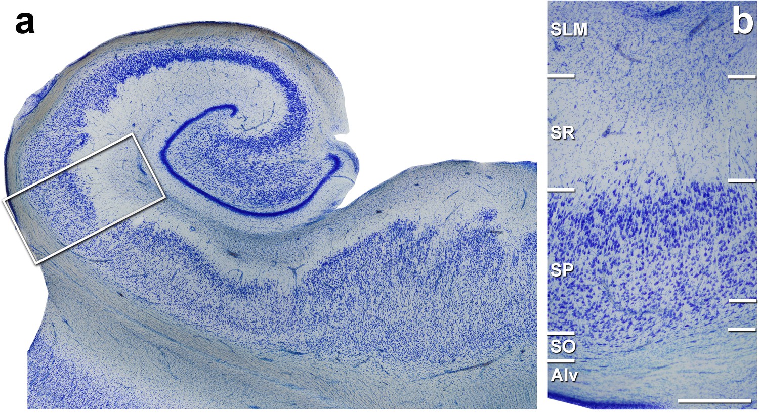
Coronal section of the human hippocampus at the level of the hippocampal body.
(a) Low-power photomicrograph of a Nissl-stained coronal brain section from human hippocampus. (b) Higher magnification image of the boxed area shown in (a) showing the medial CA1 hippocampal field. Alv: alveus; SO: stratum oriens: SP: stratum pyramidale; SR: stratum radiatum; SLM: stratum lacunosum-moleculare. Scale bar in (b) corresponds to: 1,430 μm in (a), 490 μm in (b).
Figure 1—figure supplement 2
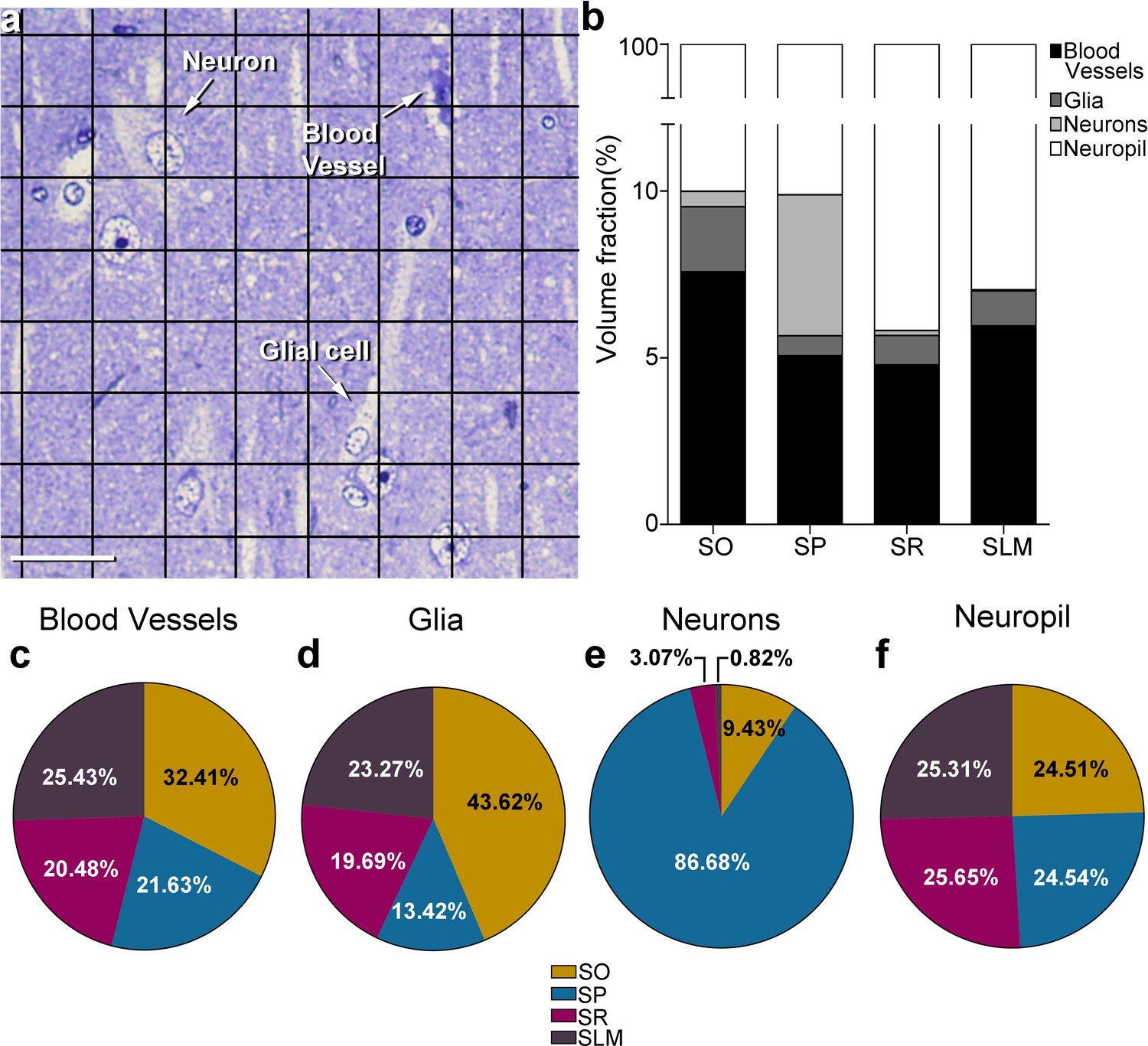
Stereological estimation of the volume occupied by different cortical elements in the CA1 using a stereological grid.
(a) Photomicrograph of a toluidine blue-stained 1 µm thick semithin section. Points hitting the different cortical elements (blood vessels, soma of glial cells and neurons) are labelled and indicated by arrows. (b) The volume fraction occupied by each cortical element in every stratum is represented with a bar chart. (c–f) Shown by pie charts the relative volume fraction including all layers of blood vessels (c), glial cells (d), neurons (e) and neuropil (f). SO: stratum oriens; SP: stratum pyramidale; SR: stratum radiatum; SLM: stratum lacunosum-moleculare. Scale bar in (a): 30 µm.
Figure 2 with 2 supplements
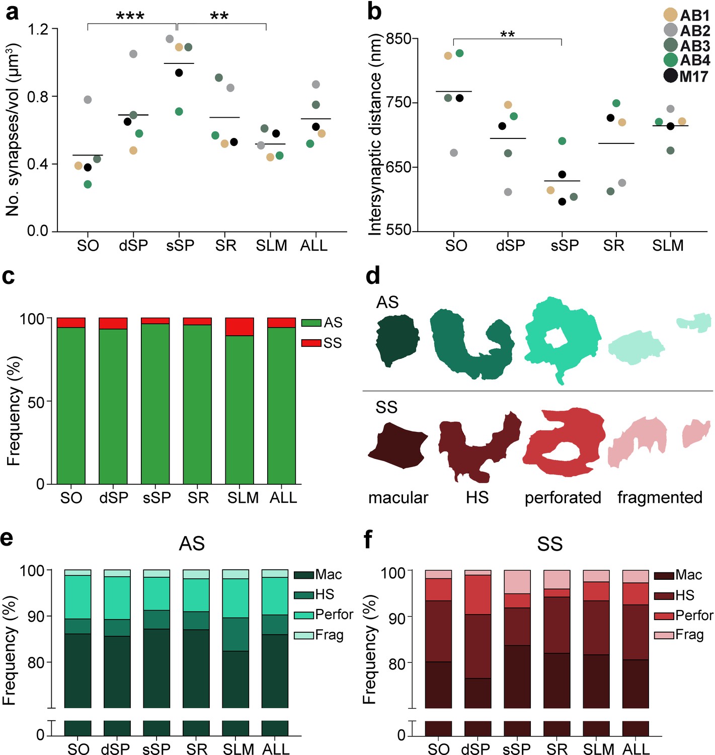
Synaptic density, intersynaptic distance, proportion of asymmetric synapses (AS) and symmetric synapses (SS), and proportion of synaptic shapes in CA1.
(a) Graph showing the mean synaptic density in all layers. (b) Graph showing the mean intersynaptic distance in all layers. Each dot in (a) and (b) represents the data from each case, with the grey line showing the mean value. (c) Shows the percentages of AS and SS in all layers. (d) Illustrates examples of the different types of synapses based on the shape of the synaptic junction: macular, horseshoe-shaped (HS), perforated and fragmented. The upper and lower rows show examples of shapes of AS and SS, respectively. (e, f) Percentages of the different types of synaptic shapes within the population of AS (e) and SS (f) in all layers. SO: stratum oriens; dSP: deep stratum pyramidale; sSP: superficial stratum pyramidale; SR: stratum radiatum; SLM: stratum lacunosum-moleculare. **p<0.01; ***p<0.001. See related Figure 2—figure supplements 1 and 2 for further information.
Figure 2—figure supplement 1

Analysis of the synaptic spatial distribution in the neuropil.
(a−e) F, G and K functions obtained in each layer: SLM (a), SR (b), sSP (c), dSP (d) and SO (e). Red dashed traces correspond to a theoretical homogeneous Poisson process for each function (F, G, K). The black continuous traces correspond to the experimentally observed function. The shaded areas represent the envelopes of values calculated from a set of 99 simulations. All plots show a distribution which fits a Poisson function in all strata which is representative of a random spatial distribution. SO: stratum oriens; dSP: deep stratum pyramidale; sSP: superficial stratum pyramidale; SR: stratum radiatum; SLM: stratum lacunosum-moleculare.
Figure 2—figure supplement 2
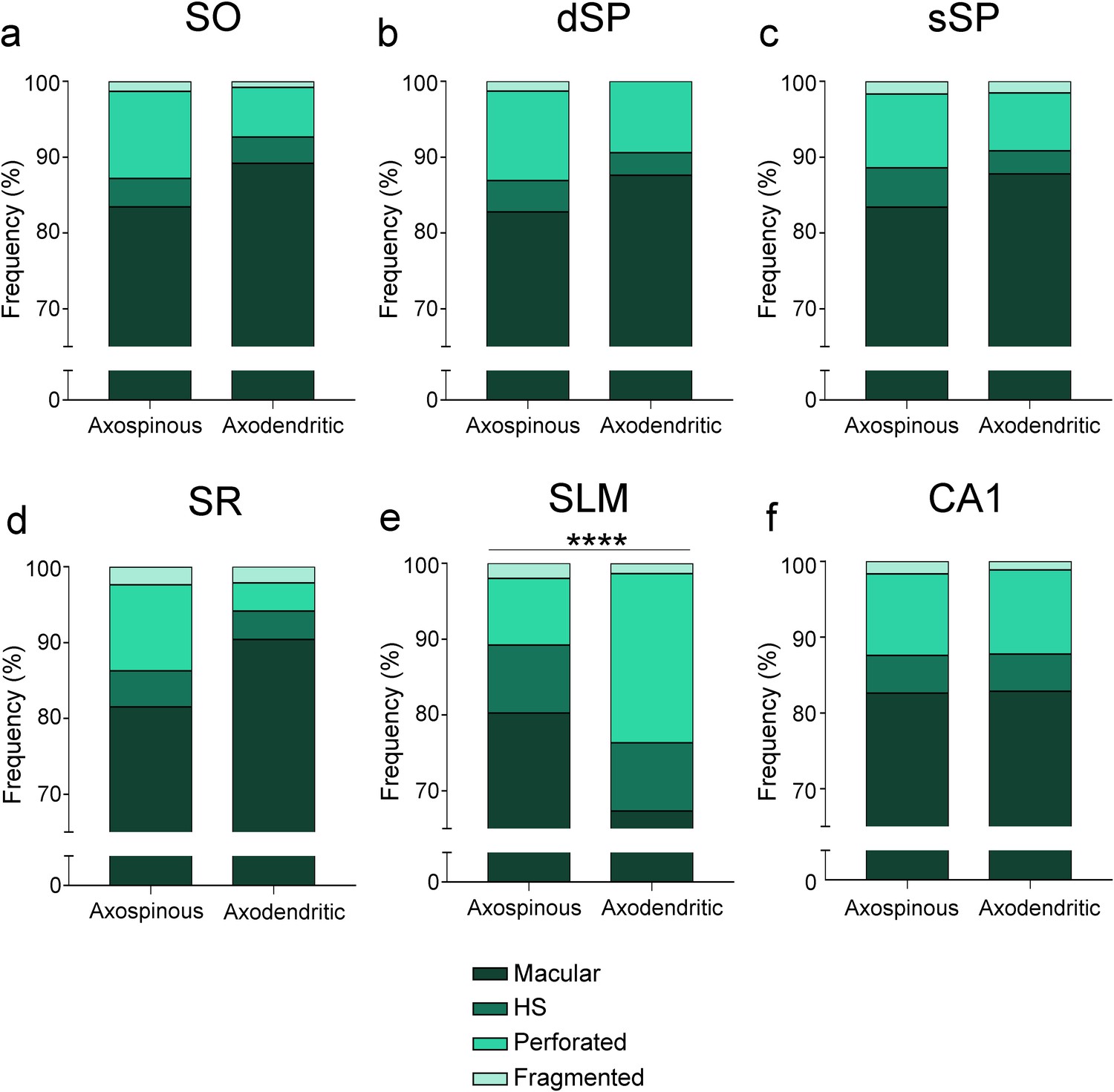
Frequency plots for every type of synaptic shape found among axospinous AS and axodendritic AS.
(a−f) Plots are shown for all layers (a−e) and for the CA1 region as a whole (f). Only in SLM, non-macular synapses are more abundant in the axodendritic AS population than in the axospinous AS one. Moreover, overall, SLM presents a higher frequency of complex-shaped synapses than other layers (see Figure 2). AS: asymmetric synapses; SO: stratum oriens; dSP: deep stratum pyramidale; sSP: superficial stratum pyramidale; SR: stratum radiatum; SLM: stratum lacunosum-moleculare. ****p<0.0001.
Figure 3
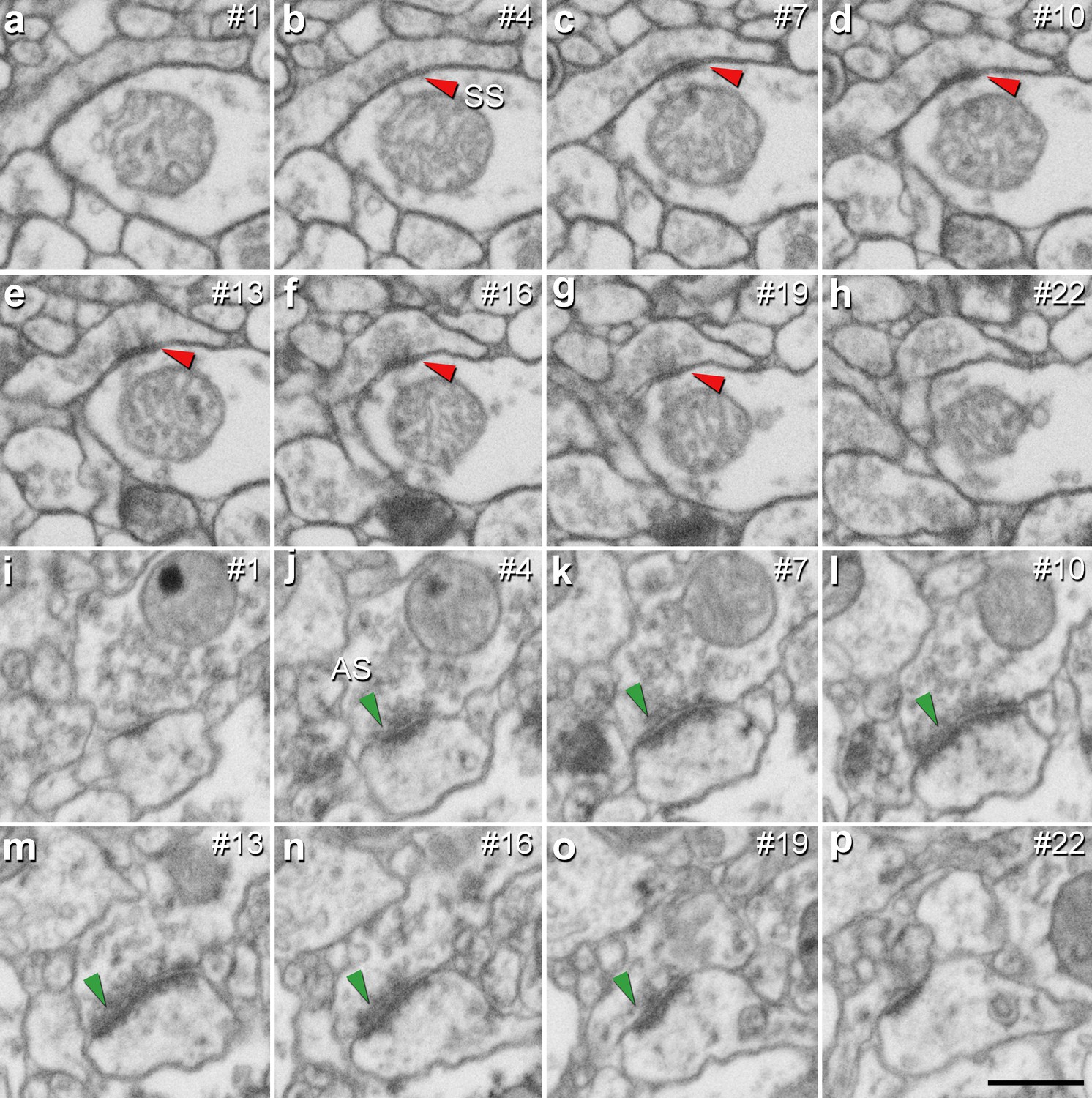
Identification of an asymmetric synapse (AS) and a symmetric synapse (SS) in the neuropil of the human CA1 region.
(a−h) Crops from electron microscopy serial sections obtained by FIB/SEM to illustrate an SS (red arrowhead). (i−p) Crops from electron microscopy images following an AS (green arrowhead). The number of the section is indicated in the top right hand corner of each section, with a 60 nm thickness separation between images. Synapse classification was based on the examination of the full sequence of serial material. Scale bar in (p) corresponds to: 500 nm in a−p.
Figure 4

Postsynaptic target identification in serial electron microscopy images.
(a) A crop from an electron microscopy section obtained by FIB/SEM to illustrate a dendritic shaft (blue) with three dendritic spines (purple) emerging from the shaft (the neck and head have been indicated in one of the spines). A symmetric synapse (SS) on the dendritic shaft is pointed out with an arrowhead. An axospinous asymmetric synapse (AS) (marked with an arrowhead) is established on the head of one of the spines. Another AS is indicated (arrowhead with asterisk); however, the nature of the postsynaptic element where the synapse is established cannot be distinguished in a single section. (b−k) Crops from electron microscopy serial sections to illustrate the nature of the postsynaptic element of the AS (arrowhead with asterisk) in (a). By following up from this AS through the stack of images (the number of the section is indicated in the top right hand corner of each section; 40 nm thickness separation between images), a dendritic spine (purple), whose neck has been labeled emerging from the dendritic shaft (blue), can be unequivocally identified. (l, m) The percentage of axospinous and axodendritic synapses within the AS (l) and SS (m) populations in all layers of CA1. SO: stratum oriens; dSP: deep stratum pyramidale; sSP: superficial stratum pyramidale; SR: stratum radiatum; SLM: stratum lacunosum-moleculare. Scale bar in (k) corresponds to: 1 µm in (a); 500 nm in (b−k).
Figure 5 with 1 supplement
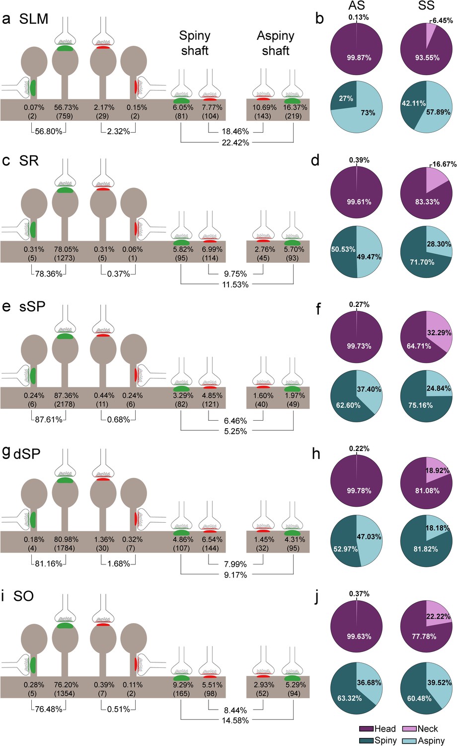
Representation of the distribution of synapses according to their postsynaptic targets in all layers of CA1.
(a, c, e, g, i) Shows the percentages of axospinous (both on the head and the neck of dendritic spines) and axodendritic (both on spiny and aspiny shafts) asymmetric synapses (AS; green) and symmetric synapses (SS; red). The numbers of each synaptic type are shown in brackets. (b, d, f, h, j) Pie charts to illustrate the proportions of AS and SS according to their location as axospinous synapses (i.e., on the head or on the neck of the spine) or axodendritic synapses (i.e., spiny or aspiny shafts). SO: stratum oriens; dSP: deep stratum pyramidale; sSP: superficial stratum pyramidale; SR: stratum radiatum; SLM: stratum lacunosum-moleculare. See related Figure 5—figure supplement 1 for further information.
Figure 5—figure supplement 1

Schematic representation of the distribution of synapses regarding postsynaptic targets and dendritic spines in the whole CA1.
(a) Frequency of axospinous synapses (both on the head and neck of dendritic spines) and axodendritic synapses (both on spiny and aspiny shafts) for asymmetric synapses (AS; green) and symmetric synapses (SS; red). Percentage and number of each synaptic type (below in brackets) are shown. (b) Proportions of the exact location of axospinous synapses (i.e., the head or neck of the spine) and axodendritic synapses (i.e., spiny or aspiny shafts) in both AS and SS, represented as pie charts. (c) Percentage of dendritic spines receiving single or multiple synaptic contacts. AS: asymmetric synapse; SS: symmetric synapse.
Figure 6 with 3 supplements
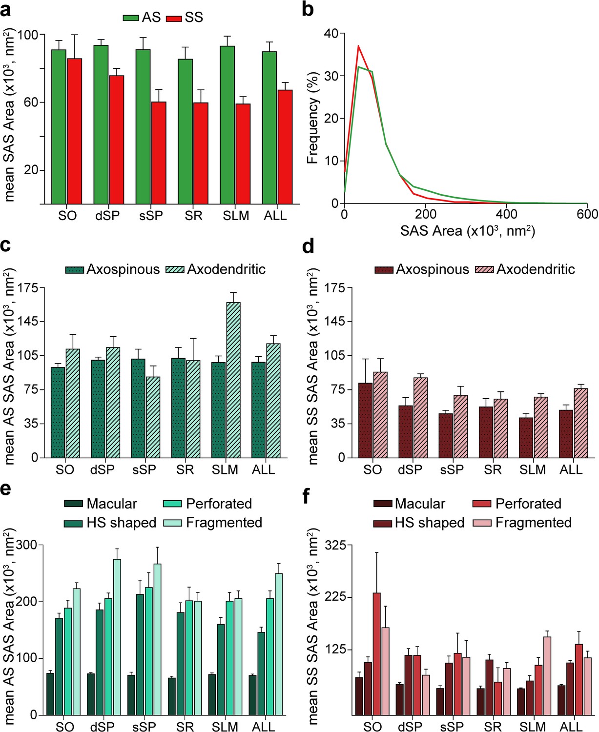
Synaptic apposition surface (SAS) area measurements from 5 subjects.
(a) Mean SAS area of asymmetric synapses (AS; green) and symmetric synapses (SS; red) are represented for each layer of CA1 (mean ± sem). (b) Frequency distribution of SAS areas for both AS (green line; n = 18,138 synapses) and SS (red line; n = 1,131 synapses) in all layers of CA1. No differences were observed in the frequency distribution of SAS areas between the two synaptic types (KS, p>0.05). (c), (d) Mean SAS area of axospinous and axodendritic synapses are also shown for AS (c) and SS (d) in the whole CA1 and per layer (mean ± sem). Both axodendritic AS and SS were larger in SLM than axospinous AS (MW, p<0.01) and SS (MW, p<0.05), respectively, while in the rest of the layers, no differences were observed. (e), (f) Mean SAS area related to the different synaptic shapes are plotted for both AS (e) and SS (f) in all layers of CA1 (mean ± sem). Macular synapses are significantly smaller than the other more complex-shaped ones (i.e., horseshoe-shaped (HS), perforated and fragmented); however, this difference is only significant for AS (ANOVA, p<0.0001). SO: stratum oriens; dSP: deep stratum pyramidale; sSP: superficial stratum pyramidale; SR: stratum radiatum; SLM: stratum lacunosum-moleculare. See related Figure 6—figure supplements 1 and 2 for further information.
Figure 6—figure supplement 1

Frequency distribution histograms of the synaptic apposition surface (SAS) area and curvature in CA1.
(a,b) Frequency distribution histograms of SAS area in all layers of CA1 for asymmetric synapses (AS) (a) and symmetric synapses (SS) (b). Note there is a clear overlap in the frequency distribution among layers both for AS and SS. (c,d) Frequency distribution histograms of SAS curvature ratio in every CA1 layer for AS (c) and SS (d). Note there is a clear overlap in the frequency distribution among layers both for AS and SS. All histograms show a positive skewness with a higher frequency of smaller values than bigger ones. SO: stratum oriens; dSP: deep stratum pyramidale; sSP: superficial stratum pyramidale; SR: stratum radiatum; SLM: stratum lacunosum-moleculare.
Figure 6—figure supplement 2
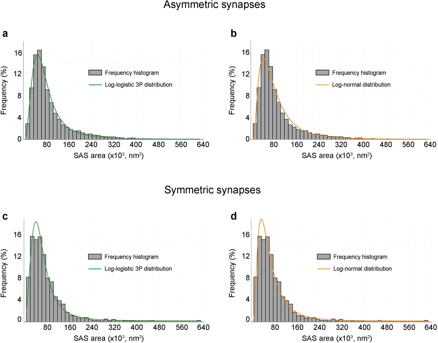
Frequency histograms of synaptic apposition surface (SAS) areas and their corresponding best-fit probability density functions.
(a,b) AS from all layers have been pooled together to build the frequency histograms (blue bars). (c,d) SS from all layers have been pooled together to build the frequency histograms (blue bars). The best-fit distributions representing the theoretical probability density functions have been represented with their corresponding frequency histograms: the log-logistic 3P (green trace) in (a, c) and the log-normal (orange trace) distribution in (b, d). Note the similarity between the log-logistic 3P and the log-normal distribution. The parameters α, β and γ of the log-logistic 3P curves and the parameters σ and μ of the log-normal curves are shown in Supplementary file 1L.
Figure 6—figure supplement 3
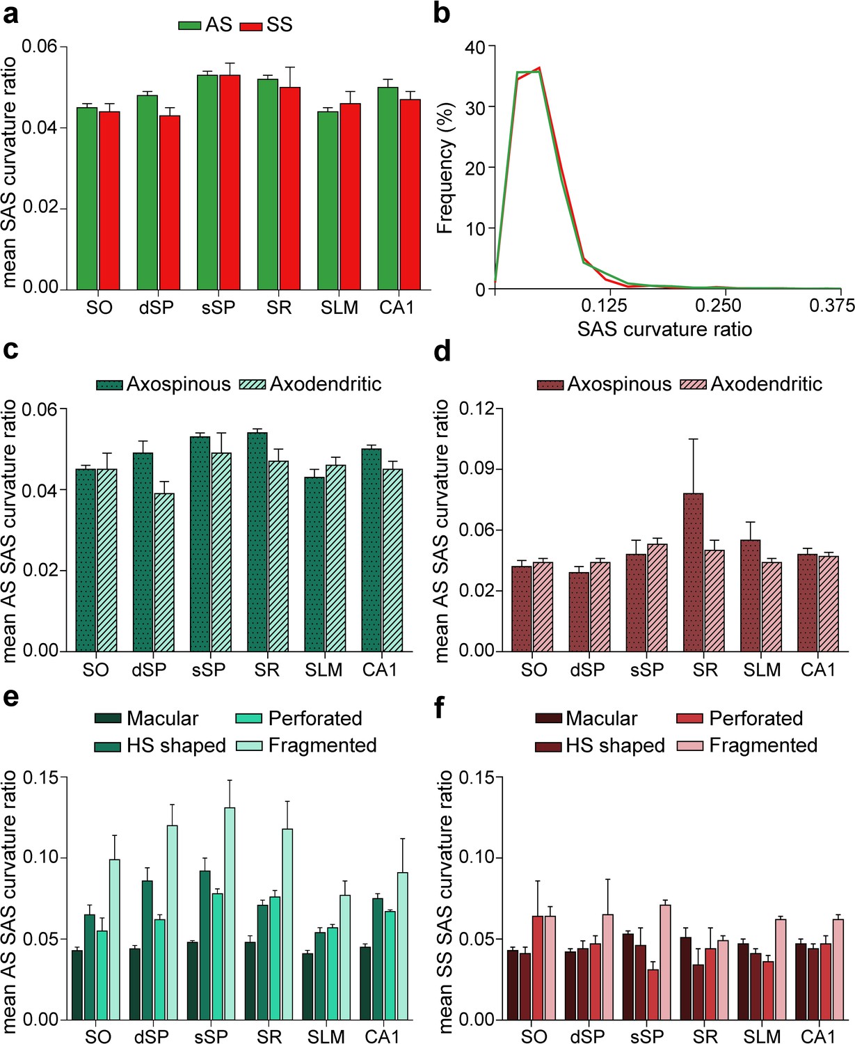
Synaptic size: synaptic apposition surface (SAS) curvature ratio from 5 subjects.
(a) Mean SAS curvature ratio of asymmetric synapses (AS) and symmetric synapses (SS) are represented for each layer and all layers of CA1 (mean ± sem). No differences were observed in the curvature ratio between AS and SS. (b) Frequency distribution of the SAS curvature ratio for AS (green line; n = 18,138 synapses) and SS (red line; n = 1,131 synapses) in all layers. Histograms show a positive skewness with a higher frequency of smaller values than bigger ones, both for AS and SS. (c,d) The mean SAS curvature of axospinous and axodendritic synapses has been plotted for AS (c) and for SS (d) in each layer and all layers (mean ± sem). No differences were observed for either AS (c) or SS (d). (e−f) The mean SAS curvature of synapses according to their shape has been plotted for AS (e) and for SS (f) in each layer and all layers (mean ± sem). Differences in the curvature ratio between the different synaptic shapes were observed. Fragmented AS were more curved than macular AS in the whole CA1 (e) — a difference that was maintained throughout all layers (ANOVA, ranged from p<0.001 to p<0.0001). Additionally, fragmented SS were more curved than the rest of the morphological types of SS (f), although this difference was only significant in SLM when taking the layers into account (ANOVA, p<0.05). Differences in the mean SAS curvature could also be observed within the same synaptic shape type between layers. In this regard, SLM presented flatter horseshoe-shaped (HS) AS than both dSP (ANOVA, p<0.01) and sSP (p<0.001), while SO exhibited flatter perforated AS than sSP and SR (ANOVA, p<0.0001). SO: stratum oriens; dSP: deep stratum pyramidale; sSP: superficial stratum pyramidale; SR: stratum radiatum; SLM: stratum lacunosum-moleculare.
Figure 7

Schematic representation of the main direct connections between CA1 and other brain regions in primates (monkeys, unless otherwise specified; note that all abbreviations are defined in the figure itself).
Photomicrograph of a Nissl-stained coronal brain section from the human CA1 (in black and white) with reconstructed pyramidal neurons (taken from Benavides-Piccione et al., 2020) superimposed on the same scale. The pyramidal neurons have been placed in the middle of the SP, approximately where they were injected with Lucifer Yellow. The apical and basal dendritic arbors are colored in blue and red, respectively. Major and minor projections have been represented with large and small arrows, respectively. See Appendix 1 for further information on human CA1 connectivity.
Tables
Table 1
Data regarding synapses in all layers of the CA1.
Data in parentheses are not corrected with the shrinkage factor. AS: asymmetric synapse; CF: counting frame; SAS: synaptic apposition surface; SD: standard deviation; SO: stratum oriens; dSP: deep stratum pyramidale; sSP: superficial stratum pyramidale; SR: stratum radiatum; SLM: stratum lacunosum-moleculare; SS: symmetric synapse.
| SO | dSP | sSP | SR | SLM | All layers | |
|---|---|---|---|---|---|---|
| No. AS | 2,648 | 3,849 | 5,183 | 3,836 | 2,622 | 18,138 |
| No. SS | 166 | 281 | 196 | 172 | 316 | 1,131 |
| No. synapses (AS+SS) | 2,814 | 4,130 | 5,379 | 4,008 | 2,938 | 19,269 |
| % AS | 94.10% | 93.20% | 96.36% | 95.71% | 89.24% | 94.13% |
| % SS | 5.90% | 6.80% | 3.64% | 4.29% | 10.76% | 5.87% |
| CF volume (µm3) | 6,221 (5,878) | 6,004 (5,486) | 5,400 (5,260) | 6,007 (5,697) | 5,690 (5,295) | 29,322 (27,616) |
| No. AS/µm3 (mean ± SD) | 0.43± 0.19 (0.45± 0.22) | 0.64± 0.22 (0.70± 0.29) | 0.96± 0.18 (0.98± 0.20) | 0.64± 0.19 (0.67± 0.22) | 0.46± 0.07 (0.49± 0.10) | 0.63± 0.21 (0.66± 0.21) |
| No. SS/µm3 (mean ± SD) | 0.03± 0.01 (0.03± 0.01) | 0.05± 0.02 (0.05± 0.02) | 0.04± 0.01 (0.04± 0.01) | 0.03± 0.01 (0.03± 0.01) | 0.06± 0.02 (0.06± 0.01) | 0.04± 0.01 (0.04± 0.01) |
| No. all synapses/µm3 (mean ± SD) | 0.45± 0.19 (0.48± 0.23) | 0.69± 0.22 (0.75± 0.31) | 0.99± 0.18 (1.02± 0.19) | 0.67± 0.19 (0.70± 0.22) | 0.52± 0.08 (0.55± 0.11) | 0.67± 0.21 (0.70± 0.21) |
| Intersynaptic distance (nm; mean ± SD) | 742.81± 63.06 (717.55± 60.92) | 669.81± 54.18 (647.04± 52.34) | 604.00± 38.08 (583.46± 36.79) | 653.77± 69.51 (637.54± 67.15) | 689.65± 23.72 (666.20 22.91) | - |
| Area of SAS AS (nm2; mean ± sem) | 86,716.52± 1,371.02 (80,906.52± 1,279.16) | 92,045.29± 1,192.92 (85,878.26± 1,112.99) | 88,061.63± 1,038.49 (82,161.50± 968.91) | 82,841.26± 1,201.47 (77,290.90± 1,120.97) | 91,419.95± 1,376.38 (85,294.81± 1,284.16) | 89,727.65± 5,775.90 (83,715.90± 5,388.91) |
| Area of SAS SS (nm2; mean ± sem) | 85,737.60± 5,869.60 (79,993.18± 5,476.62) | 74,764.69± 3,057.33 (69,755.46± 2,852.49) | 58,305.43± 2,612.01 (54,398.67± 2,437.01) | 63,183.20± 2,734.96 (58,949.93± 2,551.72) | 57,390.19± 2,071.04 (53,545.05± 1,932.38) | 67,236.17± 4,456.52 (62,731.35± 4,157.93) |
Key resources table
| Reagent type (species) or resource | Designation | Source or reference | Identifiers | Additional information |
|---|---|---|---|---|
| Chemical compound, drug | Paraformaldehyde | Sigma-Aldrich | Sigma-Aldrich: 24898648 | |
| Chemical compound, drug | Glutaraldehyde 25% EM | TAAB | TAAB: G002 | |
| Chemical compound, drug | Calcium chloride | Sigma-Aldrich | Sigma-Aldrich C2661 | |
| Chemical compound, drug | Sodium cacodylate trihydrate | Sigma-Aldrich | Sigma-Aldrich C0250 | |
| Chemical compound, drug | Osmium tetroxide | Sigma-Aldrich | Sigma-Aldrich O5500 | |
| Chemical compound, drug | Potassium ferricyanide | Probus | Probus: 23345 | |
| Chemical compound, drug | Uranyl acetate | EMS | EMS: 8473 | |
| Chemical compound, drug | Araldite | TAAB | TAAB: E201 | |
| Chemical compound, drug | Toluidine blue | Merck | Merck: 115930 | |
| Chemical compound, drug | Sodium borate | Panreac | Panreac: 141644 | |
| Chemical compound, drug | Silver paint | EMS | EMS: 12630 | |
| Software, algorithm | Stereo Investigator stereological package | MicroBrightField Inc | Version 8.0 | |
| Software, algorithm | Espina Interactive Neuron Analyzer | EspINA https://cajalbbp.es/espina | Version 2.4.1 | |
| Software, algorithm | ImageJ | ImageJ http://imagej.nih.gov/ij/ | ImageJ 1.51 | |
| Software, algorithm | GraphPad Prism | GraphPad Prism https://graphpad.com | Version 7.00 | |
| Software, algorithm | IBM SPSS Statistics for Windows | SPSS Software https://www.ibm.com/es-es/analytics/spss-statistics-software | Version 24.0 | |
| Software, algorithm | R project | R software http://www.R-project.org | Version 3.5.1 | |
| Software, algorithm | Easyfit Proffesional | Easyfit http://www.mathwave.com/es/home.html | Version 5.5 |
Additional files
-
Supplementary file 1
Supplementary tables.
- https://cdn.elifesciences.org/articles/57013/elife-57013-supp1-v1.pdf
-
Transparent reporting form
- https://cdn.elifesciences.org/articles/57013/elife-57013-transrepform-v1.pdf
Download links
A two-part list of links to download the article, or parts of the article, in various formats.
Downloads (link to download the article as PDF)
Open citations (links to open the citations from this article in various online reference manager services)
Cite this article (links to download the citations from this article in formats compatible with various reference manager tools)
Three-dimensional synaptic organization of the human hippocampal CA1 field
eLife 9:e57013.
https://doi.org/10.7554/eLife.57013


