Whole-organism behavioral profiling reveals a role for dopamine in state-dependent motor program coupling in C. elegans
- Picower Institute for Learning & Memory, Department of Brain & Cognitive Sciences, Massachusetts Institute of Technology, United States
Figures
Figure 1 with 3 supplements
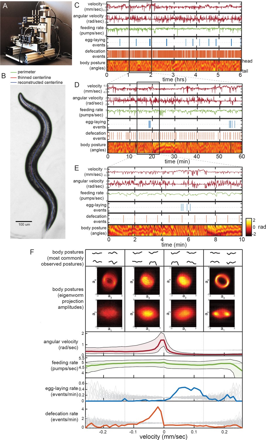
Simultaneous measurement of the diverse C. elegans motor programs.
(A) Image of the tracking microscope. (B) Example image of a C. elegans animal from the tracking microscope. Green line denotes detected outline of worm; red line indicates worm’s centerline, obtained by thinning the thresholded image; blue line is the centerline as reconstructed from a spline-based 14-parameter representation. (C–E) Example dataset from the tracking microscope, showing the main C. elegans motor programs over 6 hr (C), 1 hr (D), or 10 min (E). (F) Average behaviors observed while animals travel at different velocities. Data are from 30 wild-type animals, and data points were separated into bins based on instantaneous velocity. The average motor outputs in each bin are plotted. For angular velocity and feeding rate, data are shown as medians, as well as 25th and 75th percentiles. For egg-laying rate and defecation rate, data are shown as mean event rates (gray lines indicate random samples). For posture, data were segregated into four bins ranging from −0.25 mm/sec to 0.25 mm/sec. For each bin, we analyzed posture in two ways: by identifying and displaying the four most commonly observed postures of the 100 compendium postures described in Figure 2 (top), or by plotting 2D histograms of the projection amplitudes of the four eigenworms (middle). Eigenworm analysis was conducted using the full datasets using previously described methods (Stephens et al., 2008; and see Materials and methods) and then the projection amplitudes in each velocity bin were plotted as 2D histograms.
Figure 1—figure supplement 1
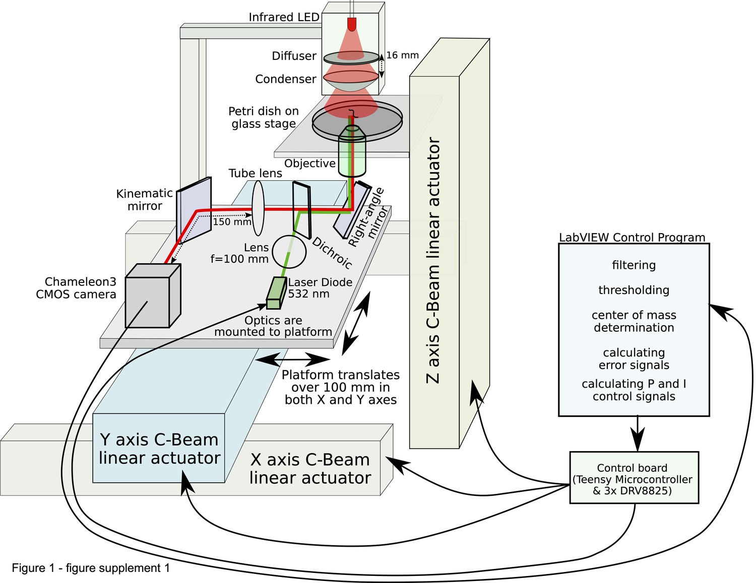
Schematic of the tracking microscope.
An infrared LED trans-illuminates the sample from above via a diffuser and a condenser lens. Light from the sample (red line) is collected by a low-magnification objective underneath the sample, and relayed via mirrors through a tube lens and finally onto a CMOS camera. For clarity, this schematic omits a dichroic mirror, laser diode, and long-pass filter enabling optogenetic stimulation or fluorescence imaging. All the optics (including the transillumination LED, diffuser, and condenser lens) are mounted on a platform that can translate over 100 mm in the X and Y axes. The stage is mounted to a third linear actuator that moves up and down, providing focusing. All linear actuators are controlled by a driver board containing three stepper driver modules (one per axis). The driver board in turn is controlled by the computer, which adjusts the microscope’s motion based on the location of the worm in the camera image. The further the worm’s center of mass is from the middle of the image, the further the microscope is instructed to move.
Figure 1—figure supplement 2
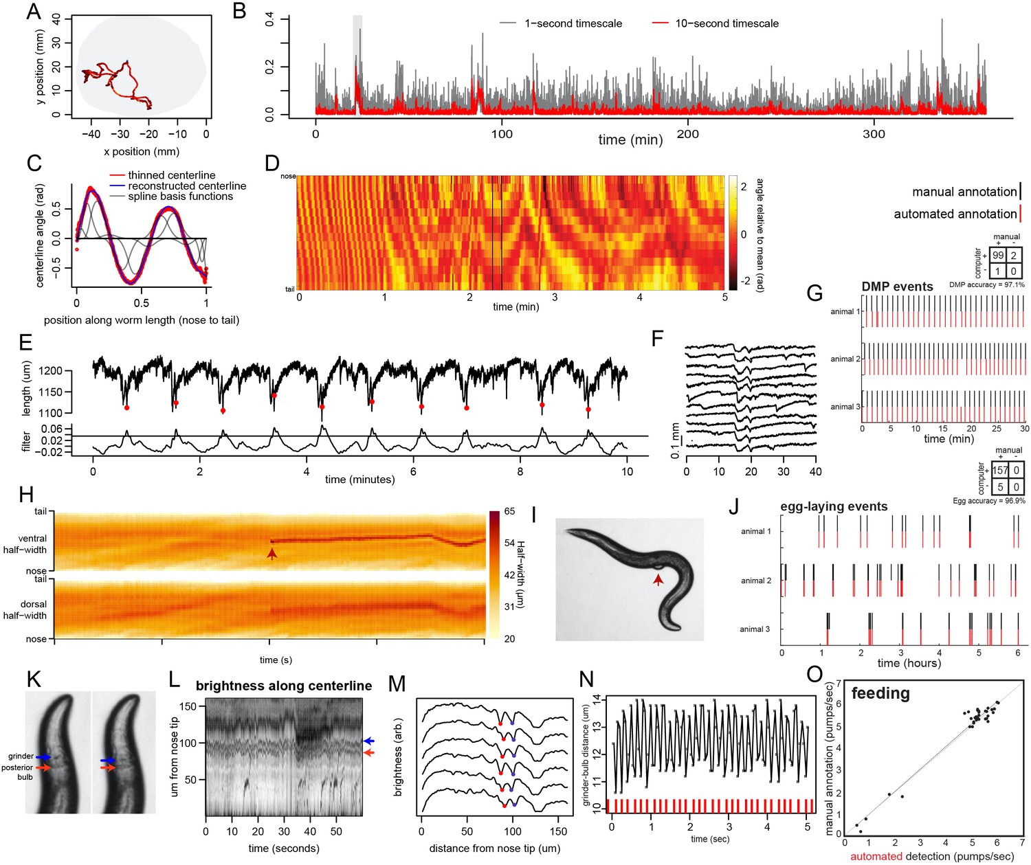
Extraction of behavioral parameters from video recordings, and validation of methods.
(A) Movement path of C. elegans animal during recording on tracking microscope. Path is color-coded by velocity (black is slow; red is fast; blue is reverse). (B) Example speed traces over a 6 hr recording of a wild-type animal. Gray shows speed calculated with a 1 s time step; red shows it calculated with a 10 s time step. (C) Body angles are accurately captured by 14-point parameterization. Data are body angles from a worm in one example frame. Centerline angles are compressed to a 14-point vector consisting of weights for a spline basis (basis functions shown as grey lines). (D) Body angles over a five-minute example dataset. Missing data (due to self-intersecting loops in body posture) are in black. (E) The defecation motor program (DMP) is detectable as a stereotyped pattern of body length contractions. Top line shows body length over 10 min. Bottom shows the data after filtering with a kernel approximating the shape of the DMP body contraction. The filter enables straightforward thresholding to detect defecation events (red dots). (F) Ten sequential defecation events are shown, revealing the stereotyped nature of body contractions during defecation events. (G) Validation of DMP detection. For three animals recorded on different microscopes, we compared the automated detection of DMP events to manual user annotation for a random 30 min segment of each video. Rasters indicate detected DMPs. Inset confusion matrix indicates accuracy. (H) Egg-laying events are detectable via instantaneous increases in body width. Example of an egg-laying event, with the widths of the dorsal and ventral sides of the body shown. Note that the width increases at the mid-body suddenly (arrowhead), reflecting the presence of an egg in this location, immediately adjacent to the animal’s body. This increase is limited to the ventral side, where the vulval muscles are located. (I) Image of a worm at the moment of an egg-laying event for the dataset in (H). (J) Validation of egg-laying detection. For three animals recorded on different microscopes, we compared the automated detection of egg-laying events to manual user annotation for all six hours of each video. Rasters indicate detected egg-laying events. Inset confusion matrix indicates accuracy. (K) Pharyngeal pumping is detected via movement of the grinder. Two sequential frames (50 ms apart) illustrating pharyngeal pumping. Pumping involves rapid retraction of the grinder, relative to the posterior end of the terminal bulb. (L) The grinder and posterior end of the terminal bulb can be detected as local minima in centerline brightness profiles. Heatmap shows brightness along the centerline for the first 160 μm of the worm’s length. Red and blue arrows show the positions of the grinder and posterior end of the terminal bulb, respectively. (M) Six sequential frames of the data in (L), plotted as line traces. Traces are offset for clarity. Red and blue dots denote the detected position of the grinder and the posterior end of the terminal bulb. (N) Pumping is clearly visible as negative peaks in the distance between the grinder and the posterior end of the terminal bulb. Plot is a time series of the distance between the grinder and posterior end of the terminal bulb, showing oscillations (pumps) at roughly 5 Hz. Red ticks at the bottom denote detected pumps. (O) Validation of pumping detection. For 35 short (20 s.) video segments (taken from 15 different recordings), we compared the automated detection of pumping rates to manual annotation by users watching videos in slow motion. R2 value is 0.9671, p<0.0001.
Figure 1—figure supplement 3
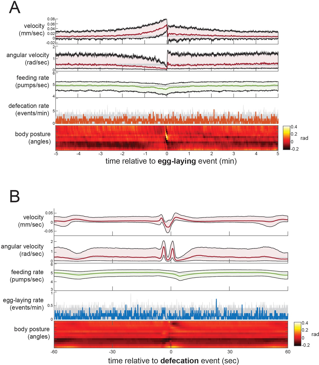
Event-triggered averages showing behavioral coordination surrounding egg-laying and DMP events.
(A) Event-triggered behavioral averages surrounding egg-laying events. Velocity, angular velocity, feeding rate, and defecation rate are shown as medians ± 25th and 75th percentiles (gray lines indicate random samples of identical size). Average body posture is shown as a heatmap of angles along the body. (B) Event-triggered behavioral averages surrounding DMP events, shown as in (A). n = 30 animals.
Figure 2 with 7 supplements
Identifying behavioral states through time series analysis of C. elegans posture.
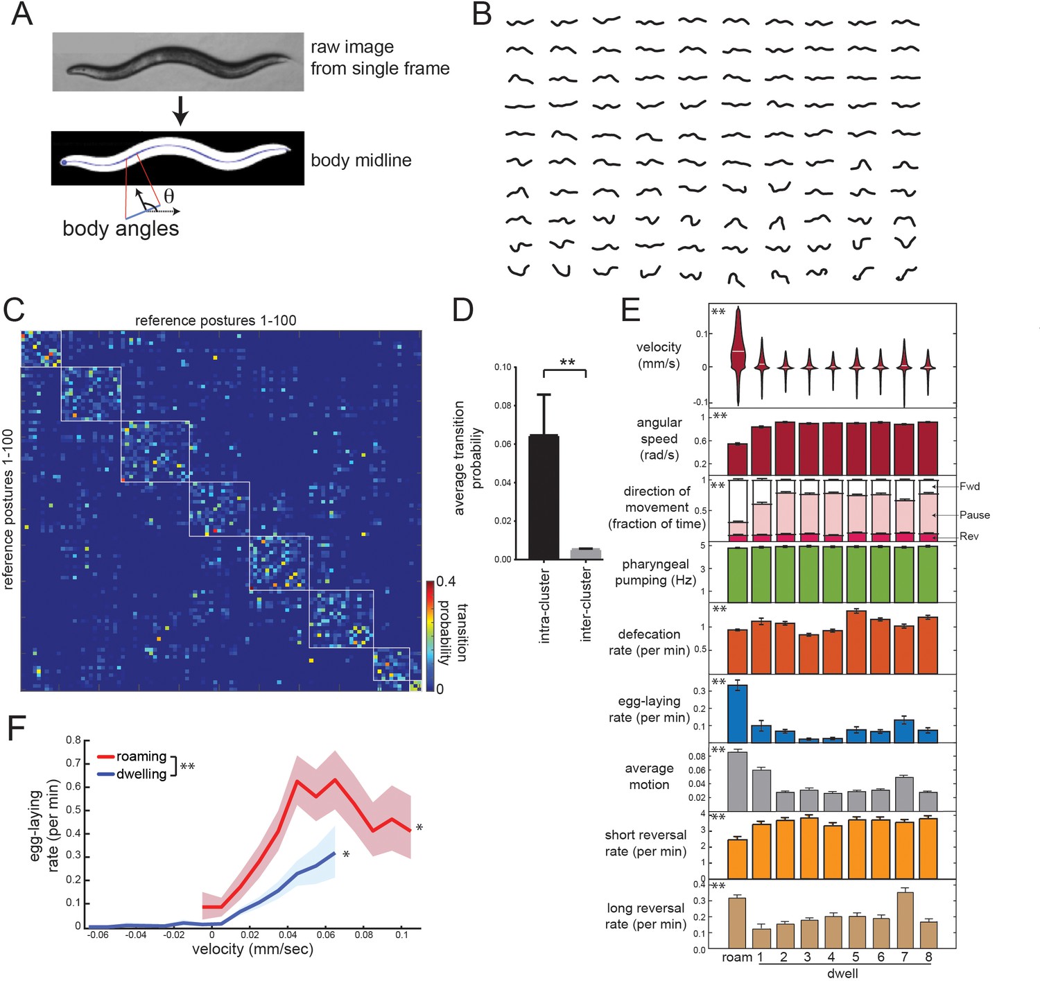
(A) Schematic showing that body posture is quantified as a vector of relative body angles, from head to tail. (B) Compendium of 100 reference postures that encompass the range of typical C. elegans postures. The compendium was derived by hierarchical clustering of many observed postures. (C) Transition matrix that shows probability of transitioning from each reference posture to the others. Self-transitions were excluded from this analysis. The rows of the matrix were clustered, and reference postures are sorted according to their cluster membership (eight clusters total; white boxes). (D) Average transition rates between postures within the same cluster, versus average transition rates between postures in different clusters. **p<0.01, Wilcoxon signed rank test. (E) Average behaviors in each hidden state. Velocity is shown as a violin plot, while other behaviors are shown as averages across 30 wild-type animals. Data are means ± standard error of the mean (SEM). ‘Average Motion’ here is defined as the average standard deviation of each of the 14 body angles over 2 s intervals throughout the state, which measures the degree to which body angles change over rapid timescales. Short reversals were backwards movements that lasted <4 s; long reversals lasted >4 s. **p<0.001, behaviors vary across states, Friedman test. (F) Average egg-laying frequency as a function of animal velocity, during roaming and dwelling states. Within each state, data points were segregated into bins based on ongoing animal velocity and egg-laying frequency was calculated across all the data points in each bin. Bins with <4 min of data per animal were excluded due to an insufficient quantity of data to warrant analysis. n = 30 animals. Error shading indicates 95% confidence intervals. **p<0.05, roaming vs dwelling, Bonferroni-corrected permutation test. *p<0.05, positive correlation of velocity versus egg-laying, empirical bootstrap test.
Figure 2—figure supplement 1
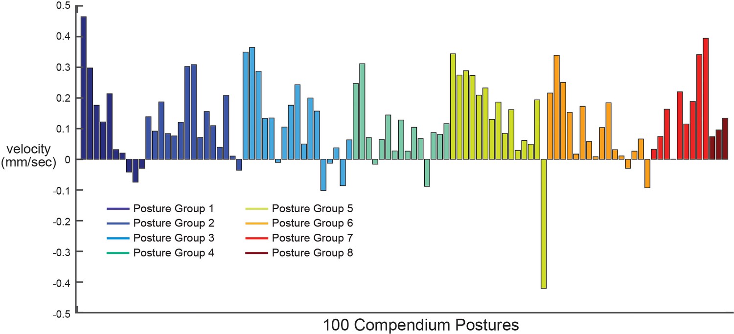
Locomotion during the 100 compendium postures.
Average animal velocity across 30 animals during each of the 100 compendium postures. Postures are ordered by posture group. Note that most posture groups (which contain different numbers of postures; see Figure 2C) contain a mixture of postures that are typically displayed during forwards and backwards movement.
Figure 2—figure supplement 2
Additional analyses related to Posture-HMM.
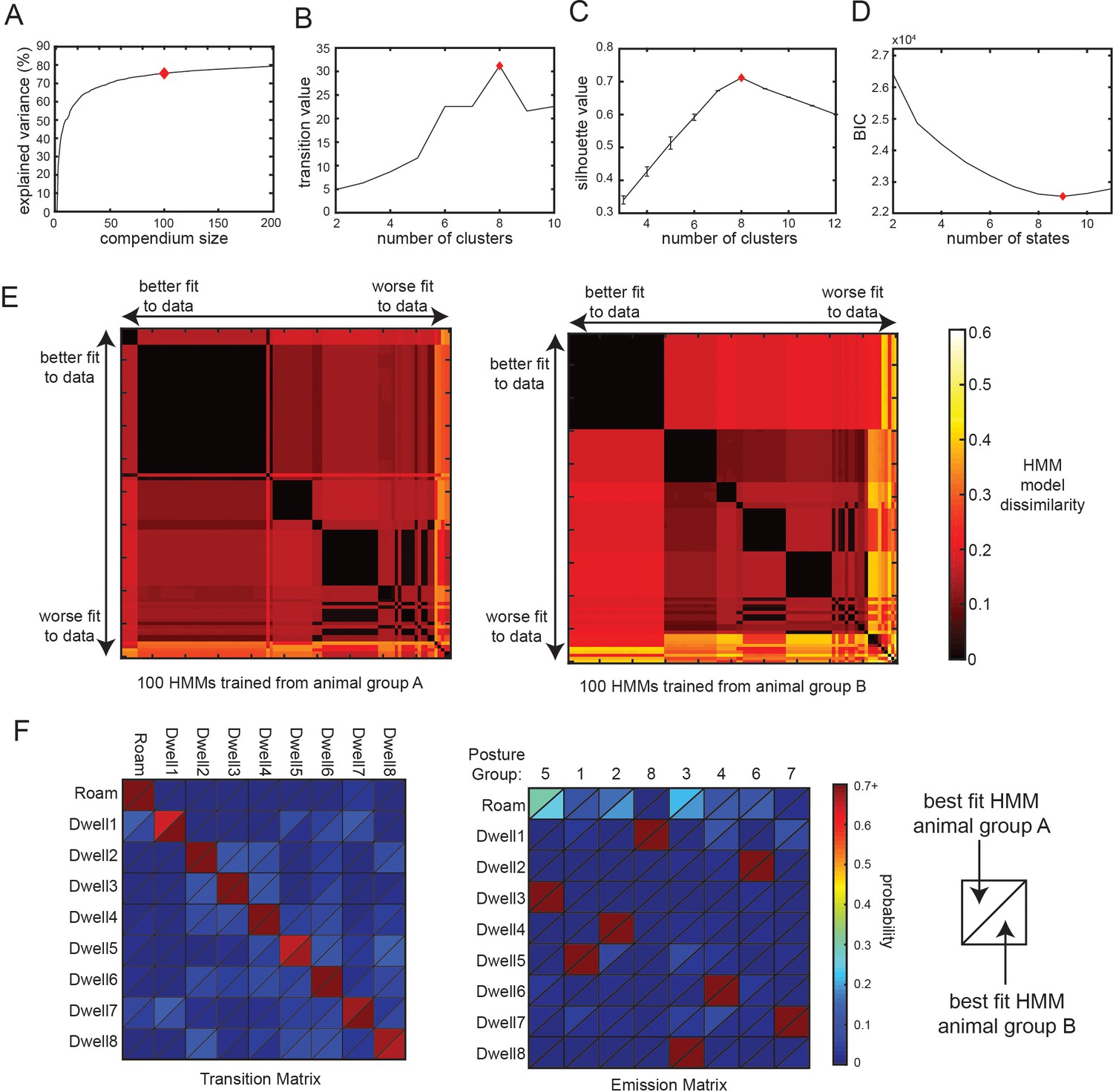
(A) A compendium of reference postures can explain most of the variance of observed animal postures. Increasing the number of postures in the compendium leads to a higher percentage of variance explained, though the impact of adding more postures diminishes gradually (i.e. plateaus). Red diamond indicates the number of reference postures used in all related analyses in this study. (B) Clustering of the transition matrix between discrete body postures maximally separates posture groups when eight clusters (red diamond) are used. ‘Transition value’ is the average intra-group (i.e. intra-cluster) transition rate divided by the average inter-group transition rate. Based on this criterion, the optimal number of clusters was eight. (C) Silhouette value when clustering the 3 s binned posture data in preparation for HMM training. Based on this criterion, the optimal number of clusters was eight. (D) BIC value for HMMs trained with varying numbers of hidden states. Based on this criterion, the best fit to the data was with a nine-state HMM. (E) These plots assess the similarity of 200 different 9-state HMMs that were trained on recorded animal data. 100 of the HMMs were trained on data from one group of animals (animal group A) and the other 100 were trained on data from a separate group of animals (animal group B). The model parameters were initialized randomly for each of the HMMs, which could in principle impact the final model parameters. The two heat maps show the dissimilarity between each pair of models trained from the two groups of animals, providing an indication of how reliably the models converged to similar parameters when they were initialized with different starting conditions. Model dissimilarity is defined here as the average Euclidean distance between the rows of the emission matrices for the two HMMs being compared. A value of 0 (black) would indicate essentially identical model parameters. The 100 HMMs from each animal group are ordered along the x- and y-axes based on their fit to the full set of wild-type data, measured as the log-likelihood of the model given the observed animal data. Note that the best fit HMMs (at the left of the x-axis; and top of the y-axis) have very similar parameters to one another (black color). This suggests that HMMs trained from different starting conditions that provided a good fit to the animal data had very similar model parameters. Panel F compares the best fit HMMs trained from each group of animals. (F) Comparison of the best fit HMMs from animal group A and animal group B shows that the training converged to a very similar solution, despite having totally independent training datasets and different random initial conditions. Data are displayed as heatmaps depicting the transition and emission matrices of the two HMMs. HMM parameters from both states are depicted in each quadrant, separated by a diagonal line (as depicted).
Figure 2—figure supplement 3
Further characterization of behavioral states from Posture-HMM.
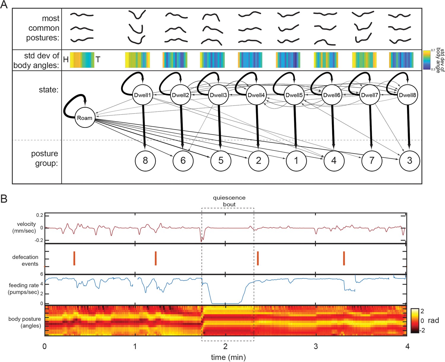
(A) Top: for each state, the most common postures observed (out of the 100 compendium reference postures; Figure 2B) while animals are in the state are shown. The postures exhibited in each of the nine states are significantly different from those exhibited in all other states (p<0.05, Bonferroni-corrected permutation test). Middle: standard deviation of body angles from head to tail across all data points where animals were in the state, providing a measure of how much the body angles vary within the state. Bottom: HMM structure learned from behavioral recordings. Arrows between states depict transition probabilities, while arrows directed to posture groups depict emission probabilities. Arrow thickness indicate probabilities. (B) An example of quiescence behavior in a wild-type animal. Although the tracking approach that we use in the study is able to identify bouts of quiescence, these bouts were extremely infrequent (five bouts detected in 30 wild-type animals recorded for six hours each) under the experimental recording conditions used here.
Figure 2—figure supplement 4
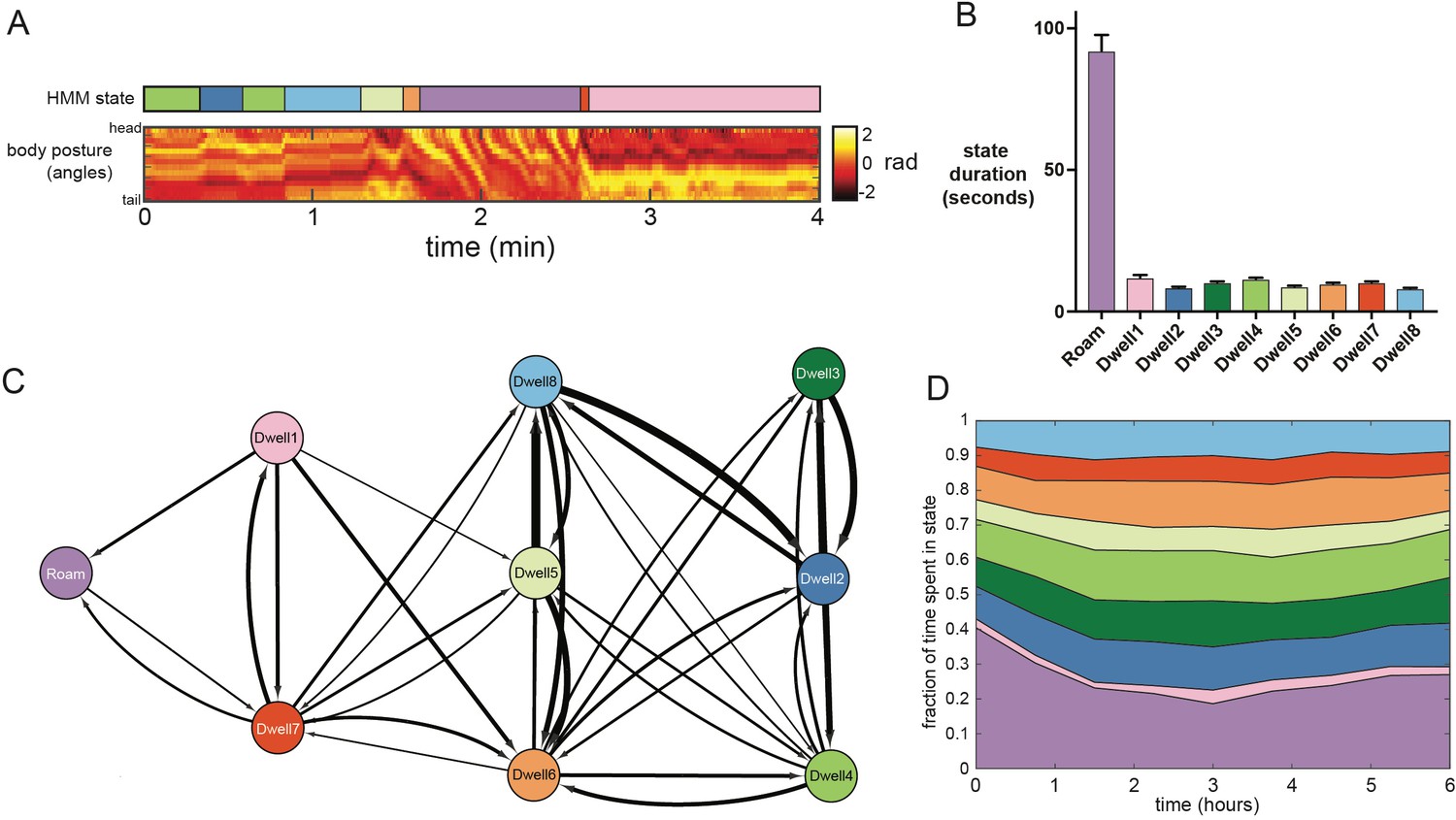
Analysis of the dwelling sub-modes.
(A) Example behavioral data from a wild-type animal showing raw posture data and an ethogram indicating the animal’s behavioral state, inferred from the posture-HMM. The color legend for the ethogram can be found in panel C. (B) Average durations of the nine HMM states. n = 30 animals. (C) Schematic indicating the transition probabilities between the nine HMM states. Arrow thickness indicates transition probability from the learned HMM parameters. For clarity, self-transitions and transitions with probabilities lower than 0.02 are excluded from the image. (D) Average time spent in each of the nine HMM states over the six hour duration of each recording. Data are averaged across 30 animals.
Figure 2—figure supplement 5
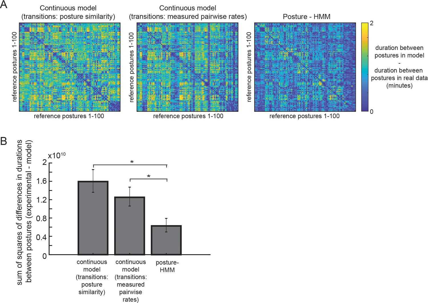
The posture-HMM generates posture sequences that resemble those from real animals.
(A) Heat maps showing the differences between synthetic posture sequences and real posture sequences for three different models of postural transitions during dwelling (see Materials and methods for full description). Each datapoint in each heatmap indicates the absolute value of the difference between synthetic data and real animal data with regards to the average duration of time between two postures (indicated by rows and columns). Lower (blue) values indicate a closer match to real animal data. Plots were constructed the same way for the three alternative models. n = 2174 observations on average for each pair of postures across all real and synthetic data. (B) Average sum of the squares of the errors for the synthetic posture sequences generated by each indicated model, as compared to real animal posture sequences. Error here is defined as the difference between synthetic data and real animal data with regards to the average duration of time between two given postures. Thus, these values are essentially the sum of the squares of the values across the entire matrices in panel A. **p<0.001, Permutation test.
Figure 2—figure supplement 6

Locomotion surrounding egg-laying events.
(A) Egg-laying rates over the durations of roaming states. All roaming states were ‘stretched’ so that they could be properly aligned (t = 0 is the onset of the roaming states), and then the normalized egg-laying rates over the durations of the states were plotted. Note that egg-laying rate are high during most of the roaming states. However, rates are not as high at the very beginnings of these state and the rates are still high for a short while after roaming states terminate. Data are from 1573 roaming states across 30 animals. (B) Event-triggered average of velocity, aligned to egg-laying events. This panel only shows data surrounding egg-laying events that were embedded in roaming states (animal roamed from −1 min to +1 min). (C) Event-triggered average of velocity, aligned to egg-laying events. This panel only shows data surrounding egg-laying events that were during dwelling states.
Figure 2—figure supplement 7
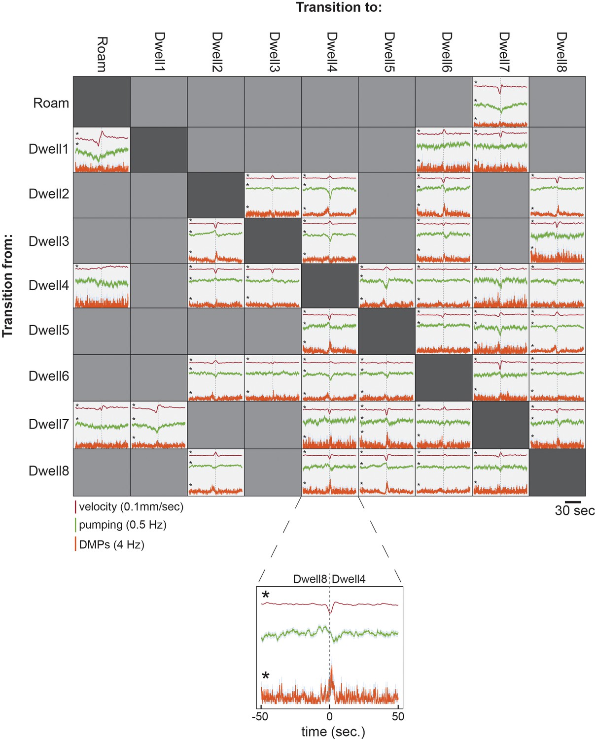
Stereotyped behavioral changes accompany state transitions.
Event-triggered averages are shown for velocity, pumping, and DMPs surrounding the moments of specific types of posture-HMM state transitions, indicated by the rows and columns. Above: we show all data for transitions where we obtained >250 examples of the state transition, so that we excluded noisy measurements. Bottom: zoomed in example of one of the event-triggered averages. Statistical analysis was performed to compare average data values surrounding state transitions (−5 s to +5 s) to random samples of behaviors typical of each state. Measured data at actual state transitions were compared to random samples to determine an empirical p-value. The p-values were multiplied by 480 to correct for the large number of comparisons (three different behaviors, 40 state transitions, two data bins before and after state transitions). *p<0.01, after Bonferroni correction. Data are from 30 wild-type animals.
Figure 3 with 2 supplements
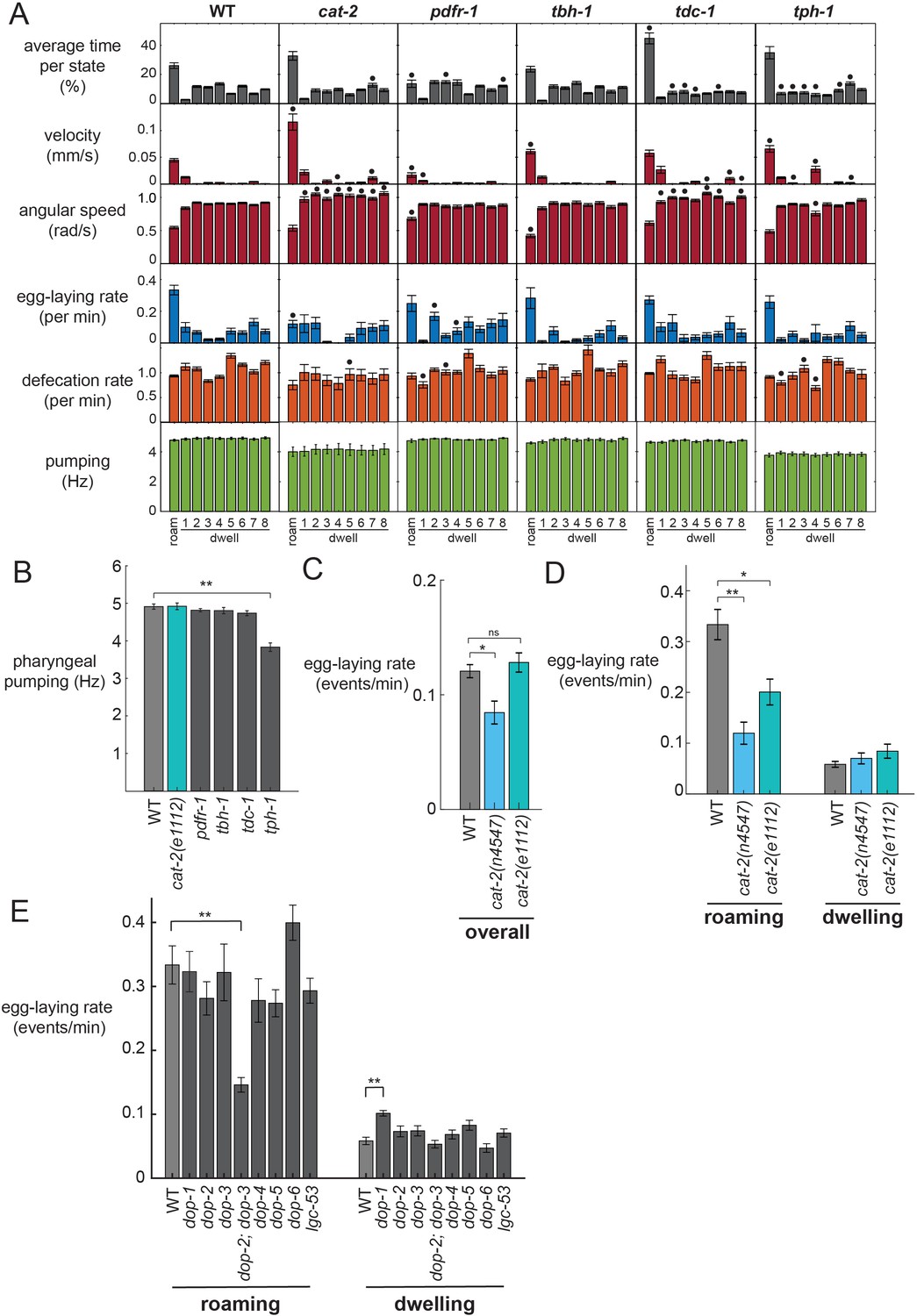
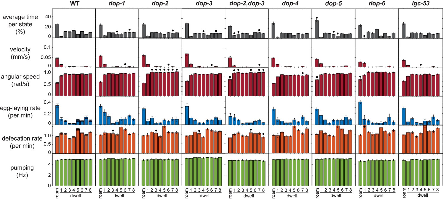
Analysis of neuromodulation mutants reveals a role for dopamine in state-dependent egg-laying.
(A) Behavioral parameters of animals of the indicated genotypes across the posture-HMM states. Black dots indicate significant changes; *p<0.05, Bonferroni-corrected Mann-Whitney U test. The cat-2 mutant displayed here is the n4547 allele. (B) On food pharyngeal pumping rates in the neuromodulation mutants (data are pooled across all states). **p<0.001, Bonferroni-corrected Mann-Whitney U test. For (A–B), n = 10–30 animals per genotype. (C) Overall egg-laying rates in the cat-2 null mutants. *p<0.01, Mann-Whitney U test. (D) Egg-laying rates during roaming and dwelling states in two different dopamine-deficient cat-2 null mutant strains. *p<0.05, Mann-Whitney U test. **p<0.001, Mann-Whitney U test. For (C–D), n = 10–30 animals per genotype. (E) Egg-laying rates during roaming and dwelling for mutant animals lacking specific dopamine receptors. **p<0.01, Bonferroni-corrected Mann-Whitney U test. n = 9–30 animals. All data are shown as means ± SEM.
Figure 3—figure supplement 1

Additional behavioral analysis of mutant strains.
(A) The postures that cat-2 mutant animals display during roaming are similar to those displayed by wild-type. Data are histograms of percent time in each of the eight posture groups during roaming for the indicated genotypes. ANOVA shows no effect of genotype on posture group prevalence. (B) Behavioral parameters across the 9-states for animals of the indicated genotypes. Black dots indicate significant changes; *p<0.05, Bonferroni-corrected Mann-Whitney U test. (C) Introduction of cat-2 genomic fragment into cat-2(n4547) mutants elevates egg-laying rates during roaming. n = 10–30 animals per genotype. †p=0.0757, Mann-Whitney U test. (D) Egg-laying rates during roaming and dwelling for egl-1 mutant animals. **p<0.001, Mann-Whitney U test. n = 21 animals for egl-1 and n = 30 animals for WT. (E) Velocity of mutant animals lacking specific dopamine receptors. n = 9–30 animals per genotype. All data are shown as means ± SEM.
Figure 3—figure supplement 2
Full behavioral parameters of the dopamine receptor mutant animals.
Behavioral parameters during each of nine HMM states are shown for animals of the indicated genotypes. Black dots indicate significant changes; *p<0.05, Bonferroni-corrected Mann-Whitney U test. All data are shown as means ± SEM.
Figure 4 with 1 supplement
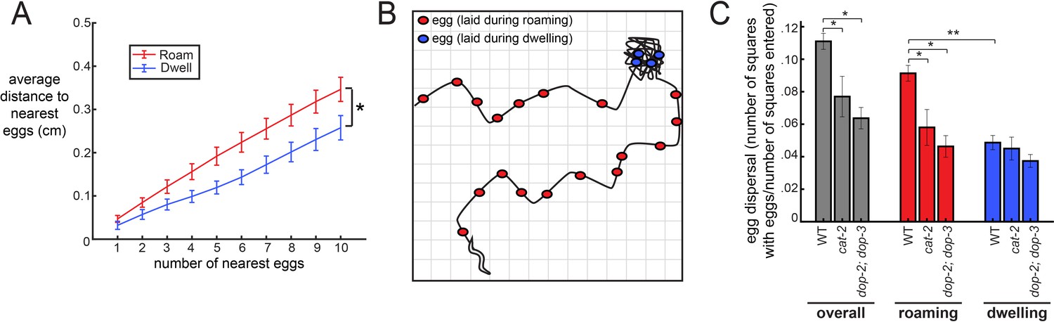
The coupling between egg-laying and roaming states leads to greater dispersal of eggs along a food source.
(A) Average distance between a given egg and its k nearest eggs for wild-type animals, separated out for eggs laid while roaming and dwelling. *p<0.01, roaming versus dwelling for all k > 3, Bonferroni-corrected Wilcoxon ranked sign test. n = 30 animals. Data are means ± SEM. (B) Schematic of the assay for egg dispersal used in panel C. A grid is virtually superimposed upon the animal’s movement path and the number of squares that contain at least one egg is counted and divided by the number of squares where the animal explored. (C) Egg dispersal overall, as well as during roaming and dwelling, for WT (n = 30), cat-2(n4547) (n = 10), and dop-2;dop-3 (n = 19), quantified as the fraction of regions explored with egg-laying events. See panel B for a schematic of the assay. Data are means ± SEM. **p<0.0001, Wilcoxon signed rank test. *p<0.05, Mann-Whitney U test.
Figure 4—figure supplement 1
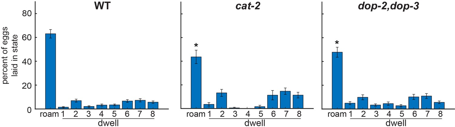
Fraction of eggs laid per state in dopamine pathway mutants.
Quantification of the fraction of eggs that were laid in each of the nine HMM states. Note that this measurement is distinct from egg-laying rate in each state, since this metric also takes into account the time spent in each state. *p<0.05, Bonferroni-corrected Mann-Whitney U test. All data are shown as means ± SEM.
Figure 5 with 1 supplement

Optogenetic control of dopaminergic neurons alters egg-laying.
(A) Inhibition of dopaminergic neurons via activation of dat-1::GtACR2 reduces egg-laying rates. Data are shown as egg-laying rates, normalized to pre-stimulation baseline rates. Gray lines show wild-type animals stimulated with the same light pattern. **p<0.0001, Wilcoxon signed rank test. (B) Average egg-laying rates during light exposure for dat-1::GtACR2 and wild-type animals. Data are shown as overall rates, as well as rates during roaming and dwelling states specifically. *p<0.05, Mann-Whitney U test. For (A–B), n = 416 light stimulation events across 12 animals for dat-1::GtACR2, and n = 769 light events across 22 animals for wild-type. (C–D) Activation of dopaminergic neurons via activation of dat-1::CoChR increases egg-laying rates. Data are shown as in (A–B). **p<0.001, Wilcoxon signed rank test. *p<0.05 Mann-Whitney U test. n = 1221 light stimulation events across 35 animals for dat-1::CoChR, and n = 769 light events across 22 animals for wild-type. (E–F) Effects of dat-1::CoChR activation in animals that are in the absence of food. Data are shown as in (A–B), except only overall egg-laying rates are shown since animals do not roam/dwell in the absence of food. *p<0.05, Mann-Whitney U test. **p<0.0001, Wilcoxon signed rank test. n = 387 light stimulation events across 44 animals for dat-1::CoChR, and n = 327 light events across 38 animals for wild-type. Data are means ± SEM.
Figure 5—figure supplement 1
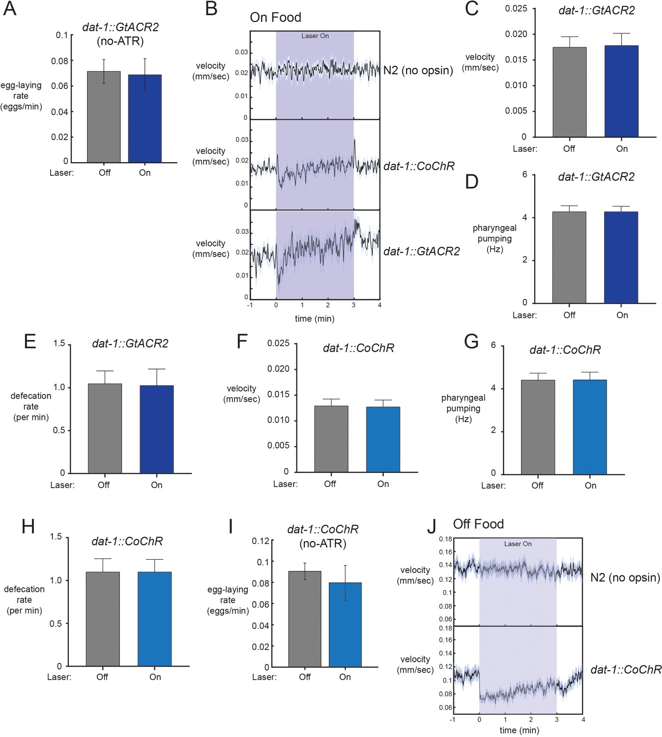
Additional optogenetic studies and analysis.
(A) No effect of laser illumination on egg-laying rates in the absence of all-trans retinal (ATR) co-factor for dat-1::GtACR2 animals. n = 12 animals. (B) Average velocity during light exposure for wild-type, dat-1::CoChR, and dat-1::GtACR2 animals for experiments conducted in the presence of food. Note that the dat-1::CoChR and dat-1::GtACR2 groups have transient changes in velocity upon light activation and termination. These changes on their own cannot explain egg-laying effects, which are persistent during the lights-on period. n = 416–1221 light stimulation events across 12–35 animals for the three genotypes. (C) Average velocity for dat-1::GtACR2 animals during lights-off and lights-on periods. n = 12 animals. (D) Average pharyngeal pumping for dat-1::GtACR2 animals during lights-off and lights-on periods. n = 12 animals. (E) Average defecation rates for dat-1::GtACR2 animals during lights-off and lights-on periods. n = 12 animals. (F) Average velocity for dat-1::CoChR animals during lights-off and lights-on periods. n = 35 animals. (G) Average pharyngeal pumping for dat-1::CoChR animals during lights-off and lights-on periods. n = 35 animals. (H) Average defecation rates for dat-1::CoChR animals during lights-off and lights-on periods. n = 35 animals. (I) No effect of laser illumination on egg-laying rates in the absence of all-trans retinal (ATR) co-factor for dat-1::CoChR animals. n = 10 animals. (J) Effects of dat-1::CoChR activation on velocity in the absence of food. Consistent with previous studies, we observe a robust reduction in speed when dopaminergic neurons are activated in the absence of food. WT control shows no effect of the light alone. n = 327–385 light stimulation events across 38–44 animals. All data are shown as means ± SEM.
Figure 6 with 1 supplement
Dopaminergic PDE neurons display activity patterns phase-locked to egg-laying during roaming.
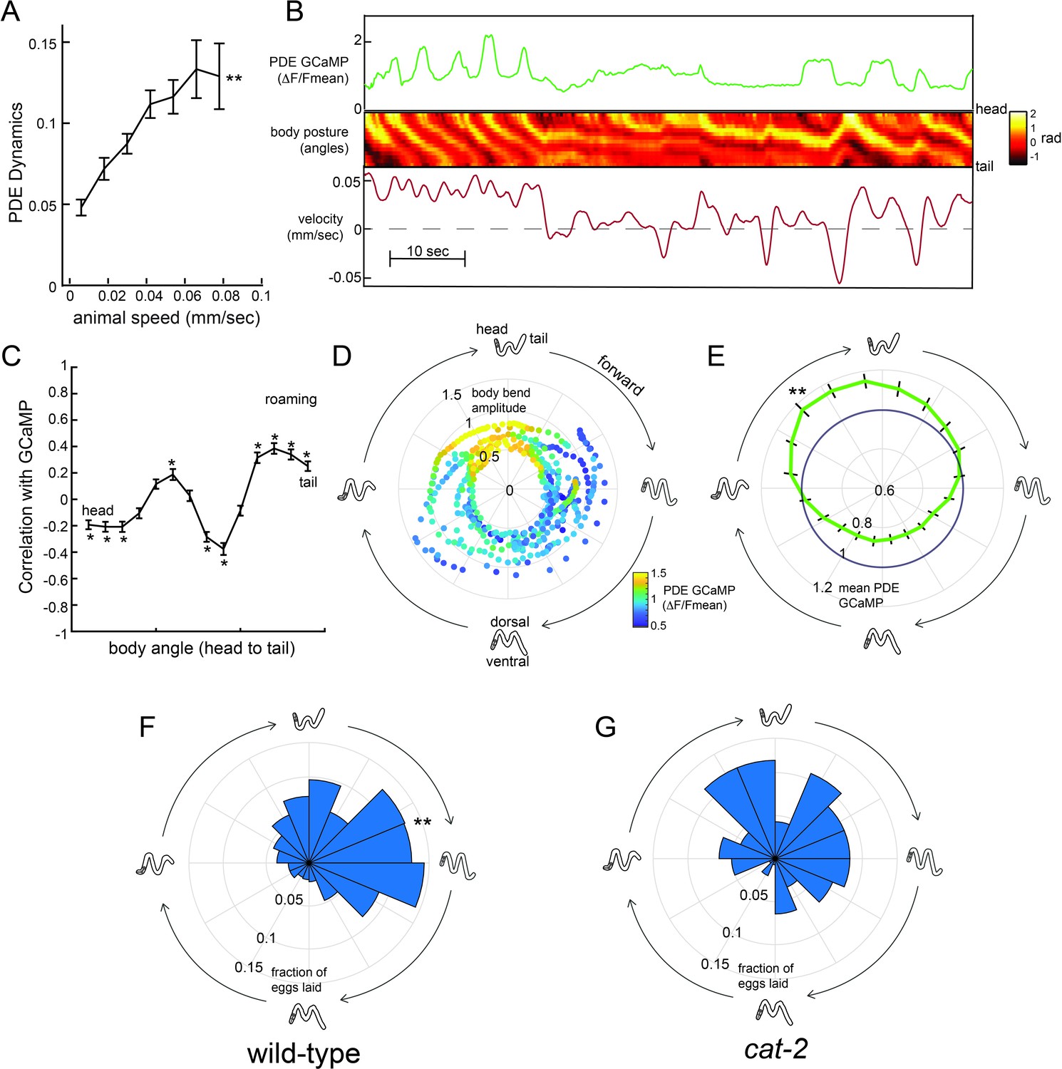
(A) PDE dynamics increase with animal speed. PDE dynamics here is defined as the absolute value of the time derivative of the PDE GCaMP signal. **p<0.001, empirical bootstrap test. (B) Example dataset from a wild-type animal, showing PDE::GCaMP6m signal, body posture (shown as body angles, from head to tail), and animal velocity. (C) Correlation coefficient of PDE activity with each of the 14 body angles. *p<0.05, empirical bootstrap test (Bonferroni-corrected). (D) Example dataset showing how PDE activity (indicated by color) changes as animals proceed through stereotyped forward propagating bends during roaming. Theta values on the polar plot correspond to the phase of the forward propagating bend; radius corresponds to the depth of the body bends (which was quantified as the standard deviation of the mean-subtracted body angles). Corresponding body postures and the direction of the trajectories during forward movement are indicated. Note that PDE activity reliably increases during a specific phase of the forward propagating bend. (E) Average PDE activity at different phases of the forward propagating bend. Theta values are defined as in (D) and the radius indicates the mean PDE GCaMP signal. **p<0.001, Mann-Whitney U test. (F) Histogram depicting frequency of egg-laying events for wild-type animals at different phases during the forward-propagating bend. **p<0.001, Rayleigh z test. (G) Histogram depicting frequency of egg-laying events for cat-2 mutants at different phases during the forward-propagating bend. *p<0.05 versus wild-type, Fisher’s exact test. For (A), (C), and (E), n = 39 animals and data are shown as means ± SEM. For (F) and (G), n = 30 and 10 animals, respectively.
Figure 6—figure supplement 1
Additional analyses related to PDE activity and egg-laying.
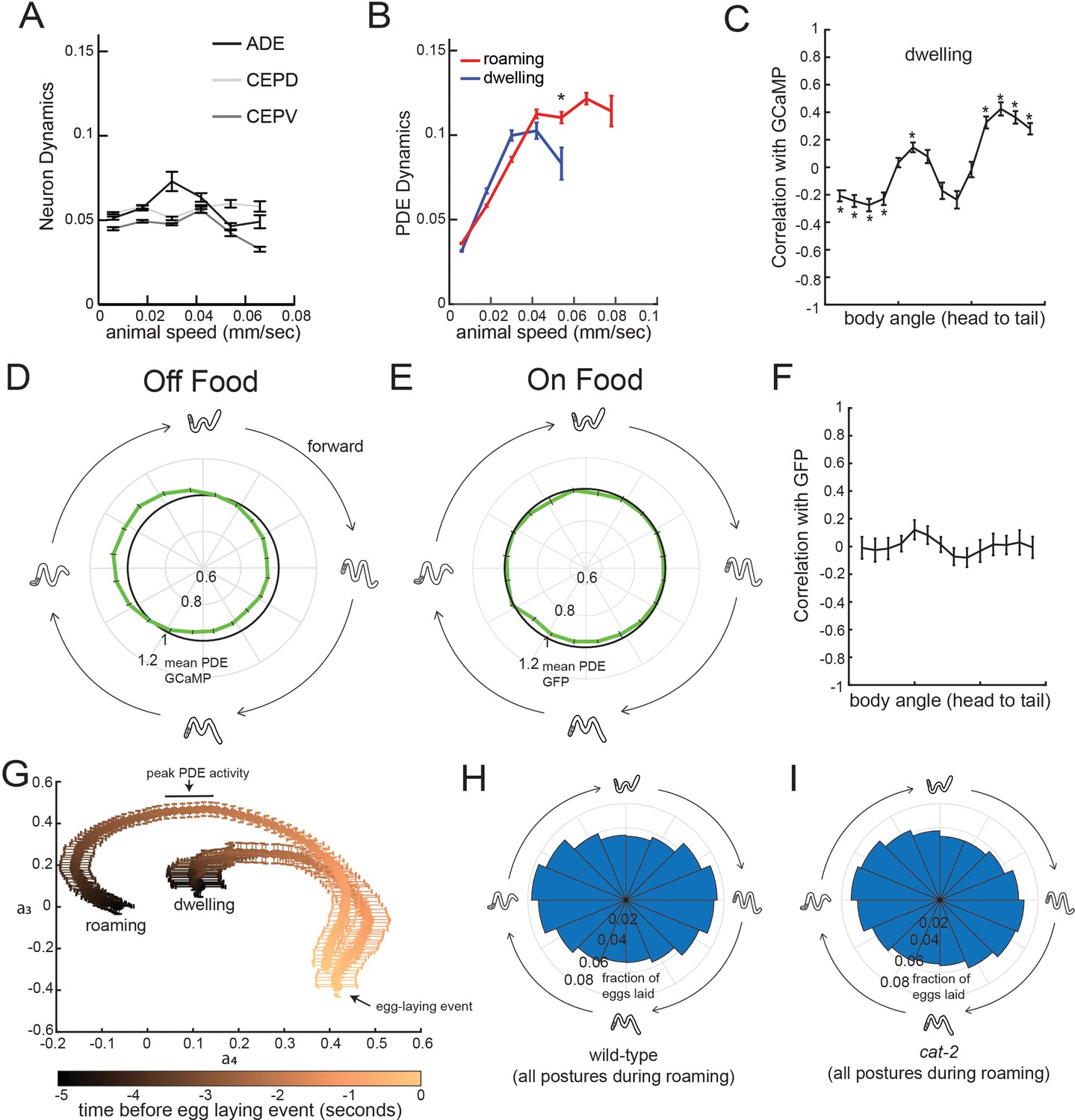
(A) Dynamics of ADE, CEPD, and CEPV do not vary with animal speed. Dynamics here is defined as the absolute value of the time derivative of the GCaMP signal for each neuron. n = 22–28 animals per condition. (B) Average PDE calcium dynamics for animals traveling at different speeds in different states. Calcium dynamics are defined here as the absolute value of the time derivative of the GCaMP signal. N = 39 animals. *p<0.001, roaming versus dwelling, Mann-Whitney U test. (C) Correlation between each of the body angles and PDE activity during dwelling states. N = 39 animals. *p<0.05, empirical bootstrap test (Bonferroni-corrected). (D) Average PDE GCaMP activity during forward-propagating bends for animals recorded in the absence of food. There is significantly reduced activity at the peak phase relative to animals on food (p<0.05, Mann-Whitney U test). n = 56 animals off food and n = 39 animals on food. (E) Average PDE GFP signal during forward-propagating bends for animals recorded in the presence of food. Compare to actual PDE::GCaMP signal in Figure 6E. n = 12. (F) Average correlations of PDE::GFP signal with body curvature. Compare to actual PDE::GCaMP signal in Figure 6C. n = 12. (G) Average postural changes for the five seconds that precede egg-laying events in roaming versus dwelling states. Data are shown as average trajectories through PCA space, where the two axes are the projection amplitudes of the third and fourth eigenworms (see Figure 1F for full 2D histograms; the third and fourth eigenworms are most relevant to undulatory locomotion). Note that the posture trajectories differ in the seconds preceding egg-laying, even though they converge to be almost the same at the moment of egg-laying. n = 30 animals. (H) Histogram depicting phases of the propagating forward bend that wild-type animals display overall, shown as same format as in Figure 6G–H. n = 30 animals. (I) Histogram depicting phases of the propagating forward bend that cat-2 mutants display overall. Note that there is no significant difference between wild-type and cat-2. n = 10 animals. For (A–G), data are shown as means ± SEM.
Figure 7
Dopamine elevates egg-laying in a GABA-dependent manner.
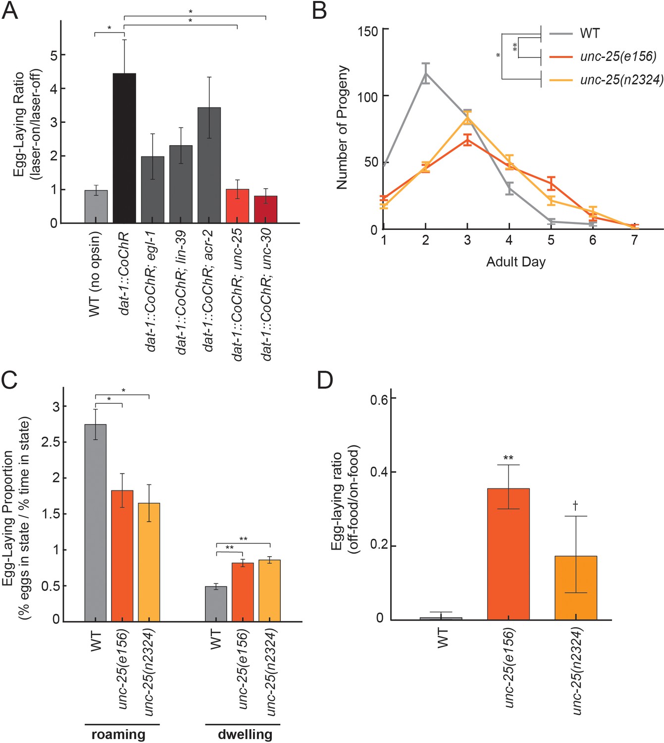
(A) Effects of dat-1::CoChR activation in genetic mutants with disrupted components of egg-laying circuitry. Data are shown as the fold increase in egg-laying during lights-on period, compared to lights-off period (a value of 1 indicates no effect of the light on egg-laying). *p<0.05, Mann-Whitney U test. n = 9–35 animals per genotype. (B) Two independent null mutants lacking unc-25, which is required for GABA synthesis, have an altered profile of egg-laying. Data are shown as average eggs laid per day, with the first day being the first 24 hr after L4. *p<0.05 and **p<0.01, effect of genotype in two-factor ANOVA and post-hoc pairwise Dunnett test. n = 5–10 animals per genotype. (C) Percent of eggs laid during roaming and dwelling for two independent null mutants of unc-25, which are defective in GABA synthesis. Here, we display data in this format to normalize for the reduced brood size in unc-25. *p<0.05, Mann-Whitney U test. **p<0.001, Mann-Whitney U test. n = 11–30 animals per genotype. (D) Egg-laying in the absence of food is elevated in unc-25 mutants. Data are shown as a ratio of eggs laid off food divided by eggs laid on food. **p<0.01 and †p<0.1 in ANOVA and post-hoc pairwise Dunnett test. n = 5–6 plates per genotype, each with 10 animals per plate.
Videos
Video 1
Examples of behavioral states captured through posture-HMM.
This video shows examples of the nine different behavioral states identified through posture-HMM. Note that videos are of different durations and are looped.
Tables
Key resources table
| Reagent type (species) or resource | Designation | Source or reference | Identifiers | Additional information |
|---|---|---|---|---|
| Strain, strainbackground (E. coli) | OP50 | CGC | ID_FlavellDatabase:OP50 | OP50 |
| Strain, strainbackground (C. elegans) | MT13113 | CGC | ID_FlavellDatabase: MT13113 | tdc-1(n3419) |
| Strain, strainbackground (C. elegans) | MT15620 | CGC | ID_FlavellDatabase: MT15620 | cat-2(n4547) |
| Strain, strainbackground (C. elegans) | MT9455 | CGC | ID_FlavellDatabase: MT9455 | tbh-1(n3247) |
| Strain, strainbackground (C. elegans) | CX11078 | Stern et al., 2017 | ID_FlavellDatabase: CX11078 | cat-2(e1112) |
| Strain, strainbackground (C. elegans) | CX14295 | CGC | ID_FlavellDatabase: CX14295 | pdfr-1(ok3425) |
| Strain, strainbackground (C. elegans) | LX645 | CGC | ID_FlavellDatabase: LX645 | dop-1(vs100) |
| Strain, strainbackground (C. elegans) | LX702 | CGC | ID_FlavellDatabase: LX702 | dop-2(vs105) |
| Strain, strainbackground (C. elegans) | LX703 | CGC | ID_FlavellDatabase: LX703 | dop-3 (vs106) |
| Strain, strainbackground (C. elegans) | LX704 | CGC | ID_FlavellDatabase: LX704 | dop-2(vs105); dop-3(vs106) |
| Strain, strainbackground (C. elegans) | SWF261 | this study | ID_FlavellDatabase: SWF261 | dop-4(ok1321); backcrossed to N2 8x |
| Strain, strainbackground (C. elegans) | CX13111 | this study | ID_FlavellDatabase: CX13111 | dop-5(ok568); backcrossed to N2 3x |
| Strain, strainbackground (C. elegans) | RB1680 | CGC | ID_FlavellDatabase: RB1680 | dop-6(ok2070) |
| Strain, strainbackground (C. elegans) | MT1082 | CGC | ID_FlavellDatabase: MT1082 | egl-1(n487) |
| Strain, strainbackground (C. elegans) | SWF266 | this study | ID_FlavellDatabase: SWF266 | lgc-53(n4330); MT13952 was backcrossed to N2 4x |
| Strain, strainbackground (C. elegans) | SWF181 | this study | ID_FlavellDatabase: SWF181 | cat-2(n4547), flvEx87[cat-2 genomic PCR product, myo-3::mCherry] |
| Strain, strainbackground (C. elegans) | SWF325 | this study | ID_FlavellDatabase: SWF325 | flvEx133[dat-1::GtACR2-t2a-GFP,myo-3::mCherry] |
| Strain, strainbackground (C. elegans) | SWF141 | this study | ID_FlavellDatabase: SWF141 | flvEx74[dat-1::CoChR, myo-3::mCherry] |
| Strain, strainbackground (C. elegans) | SWF207 | this study | ID_FlavellDatabase: SWF207 | egl-1(n487); flvEx74[dat-1::CoChR, myo-3::mCherry] |
| Strain, strainbackground (C. elegans) | SWF208 | this study | ID_FlavellDatabase: SWF208 | lin-39(n709); flvEx74[dat-1::CoChR, myo-3::mCherry] |
| Strain, strainbackground (C. elegans) | SWF258 | this study | ID_FlavellDatabase: SWF258 | acr-2(n2595 n2420); flvEx74[dat-1::CoChR, myo-3::mCherry] |
| Strain, strainbackground (C. elegans) | SWF257 | this study | ID_FlavellDatabase: SWF257 | unc-25(e156); flvEx74[dat-1::CoChR, myo-3::mCherry] |
| Strain, strainbackground (C. elegans) | SWF314 | this study | ID_FlavellDatabase: SWF314 | unc-30(e191); flvEx74[dat-1::CoChR, myo-3::mCherry] |
| Strain, strainbackground (C. elegans) | SWF331 | this study | ID_FlavellDatabase: SWF331 | flvEx127[dat-1::GCaMP6m, myo-3::mCherry] |
| Strain, strainbackground (C. elegans) | BZ555 | CGC | ID_FlavellDatabase: BZ555 | egIs1 [dat-1::GFP] |
| Strain, strainbackground (C. elegans) | CX14453 | Bendesky et al., 2012 | ID_FlavellDatabase: CX14453 | unc-25(n2324) |
| Strain, strainbackground (C. elegans) | CX13851 | Bendesky et al., 2012 | ID_FlavellDatabase: CX13851 | unc-25(e156) |
| Recombinant DNA reagent | pYCH1 | this study | ID_FlavellDatabase: pYCH1 | dat-1::GtACR2-sl2-GFP |
| Recombinant DNA reagent | pSKY1 | this study | ID_FlavellDatabase: pSKY1 | dat-1::CoChR |
| Recombinant DNA reagent | pSKY2 | this study | ID_FlavellDatabase: pSKY2 | dat-1::GCaMP6m |
| Software, algorithm | ImageJ | ImageJ (http://imagej.nih.gov/ij/) | RRID:SCR_003070 | Version 1.52 |
| Software, algorithm | GraphPad Prism | GraphPad Prism (graphpad.com) | RRID:SCR_002798 | Version 7.03 |
| Software, algorithm | MATLAB | MathWorks (www.mathworks.com) | RRID:SCR_001622 | Version 2019a |
| Software, algorithm | National Instruments | LabView (www.ni.com/en-us/shop/labview.html) | RRID:SCR_014325 | Version 16.0 |
| Software, algorithm | NIS Elements | Nikon (www.nikoninstruments.com/products/software) | RRID:SCR_014329 | V4.51.01 |
| Software, algorithm | The R Project | R (r-project.org) | RRID:SCR_001905 | v3.6.1 |
| Software, algorithm | R Studio | R Studio (rstudio.com) | RRID:SCR_000432 | v1.2.1335 |
Additional files
-
Supplementary file 1
Details about statistical tests.
This excel sheet includes a detailed description of each statistical test carried out in this study.
- https://cdn.elifesciences.org/articles/57093/elife-57093-supp1-v2.xlsx
-
Transparent reporting form
- https://cdn.elifesciences.org/articles/57093/elife-57093-transrepform-v2.pdf
Download links
A two-part list of links to download the article, or parts of the article, in various formats.
Downloads (link to download the article as PDF)
Open citations (links to open the citations from this article in various online reference manager services)
Cite this article (links to download the citations from this article in formats compatible with various reference manager tools)
Whole-organism behavioral profiling reveals a role for dopamine in state-dependent motor program coupling in C. elegans
eLife 9:e57093.
https://doi.org/10.7554/eLife.57093


