Integrative frontal-parietal dynamics supporting cognitive control
- Department of Psychology, Florida State University, United States
Figures
Figure 1
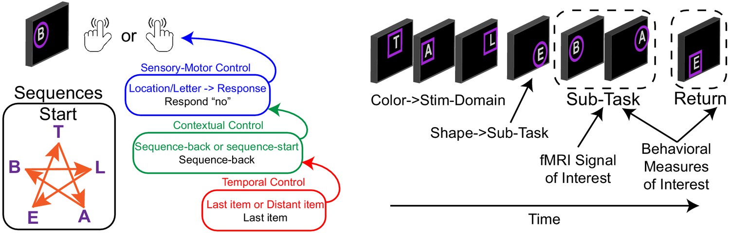
Comprehensive control task.
On each trial, participants observed a letter at a spatial location and made a keypress in response. Keypresses mapped onto ‘yes’/'no' responses. Participants either responded ‘no’ to the stimulus without regard to the stimulus features, or made a choice response based on a pre-learned sequence to a color cued feature (T-A-B-L-E-T for letters; star trace for locations) thereby engaging sensory-motor control. The correct response was either based upon a reference stimulus for which participants responded regarding whether the present stimulus followed a reference stimulus (sequence-back), or whether the stimulus was the start of the sequence (sequence-start). Switching among these tasks engages contextual control. Finally, the reference stimulus could either be the last item presented, or a distant item. In the latter case, the reference item had to be sustained over several trials requiring temporal control to prepare for the future. Colored frames indicated relevant stimulus features (letter or location), whereas frame shapes indicated cognitive control demands which were manipulated in the middle of each block (sub-task). Stimulus domain and cognitive control demands were independently manipulated in a factorial design wherein orthogonal contrasts separately isolated sensory-motor control, contextual control, and temporal control. Refer to the Materials and methods and Nee and D'Esposito, 2016; Nee and D'Esposito, 2017 for a more complete description.
Figure 2 with 2 supplements
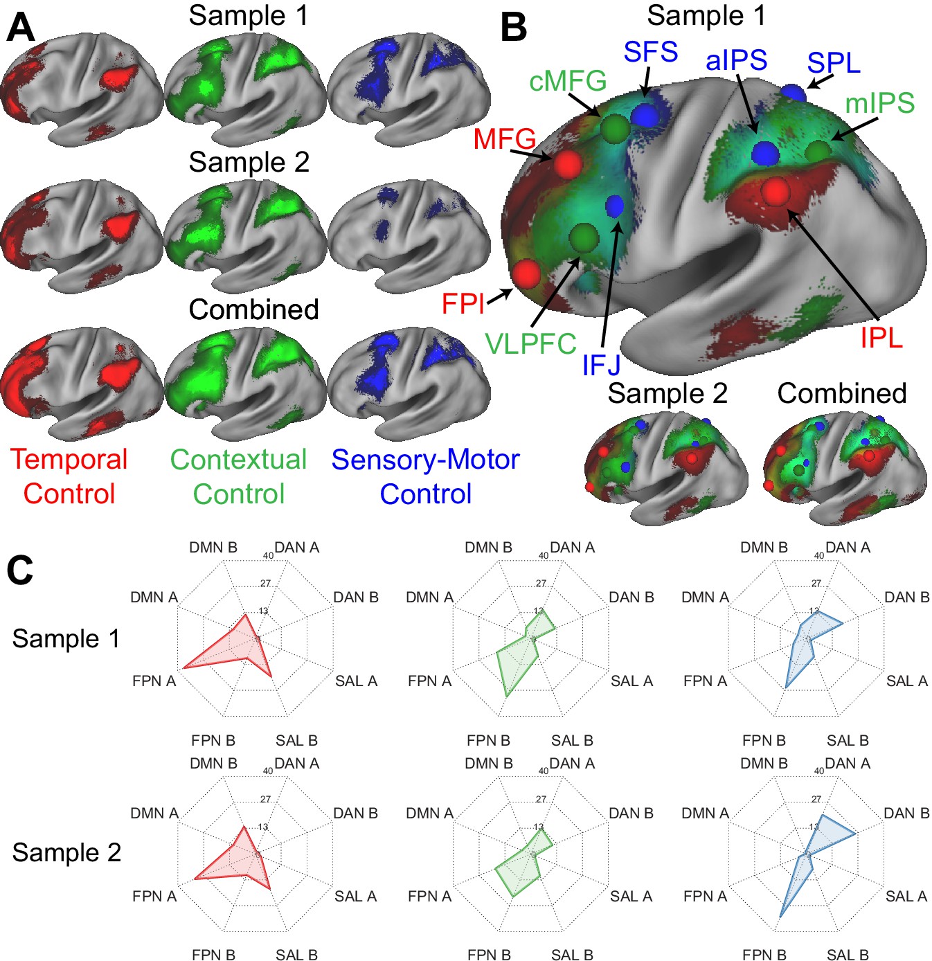
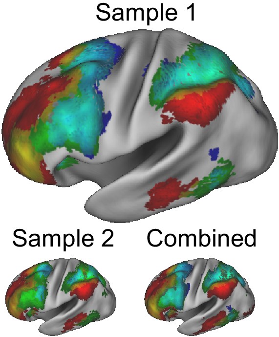
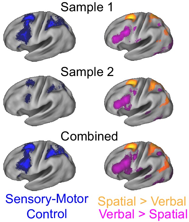
Control sub-networks.
(A) Activations for temporal control (red), contextual control (green), and sensory-motor control (blue). Activations are depicted separately for each sample, as well as the samples combined. (B) Activations overlaid to demonstrate the gradient of cognitive control. Spheres indicate the location of regions-of-interest based upon activation peaks. (C) Overlap between activation contrasts (red – temporal control; green – contextual control; blue – sensory-motor control) and the 17-network parcellation described by Yeo et al. FPl – lateral frontal pole; MFG – middle frontal gyrus; VLPFC – ventrolateral prefrontal cortex; cMFG – caudal middle frontal gyrus; IFJ – inferior frontal junction; SFS – superior frontal sulcus; aIPS – anterior intra-parietal sulcus; IPL – inferior parietal lobule; mIPS – mid intra-parietal sulcus; SPL – superior parietal lobule; DMN – default-mode network; DAN – dorsal attention network; SAL – salience network; FPN – frontoparietal network.
Figure 2—figure supplement 1
Contrasts of temporal control (red), contextual control (green), and sensory-motor control (blue) and their overlap using reduced, 4 mm full-width half-maximum volumetric smoothing to reduce blurring.
Figure 2—figure supplement 2
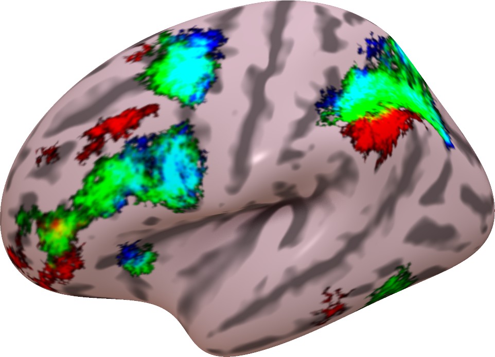
Contrasts of temporal control (red), contextual control (green), and sensory-motor control (blue) and their overlap using surface-based processing and reduced smoothing to minimize blurring.
Figure 3 with 1 supplement
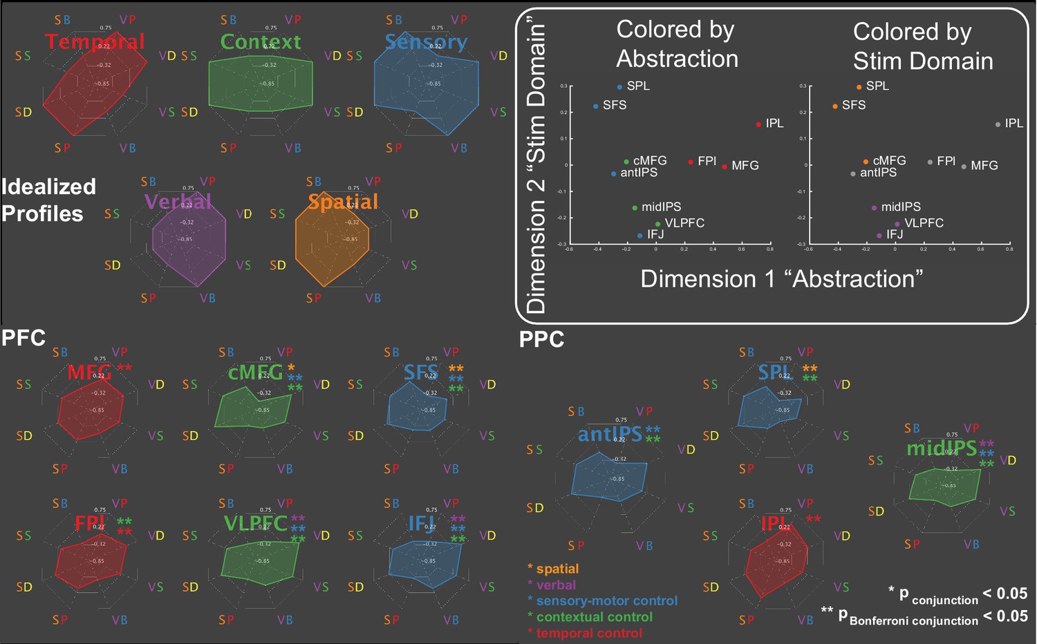
Activation profiles.
Activations across the eight conditions of the task design are depicted as radar plots (SB – spatial baseline; VB – verbal baseline; SS – spatial switching; VS – verbal switching; SP – spatial planning; VP – verbal planning; SD – spatial dual; VD – verbal dual). The top panel depicts idealized profiles for areas sensitive solely to temporal control (red), contextual control (green), sensory-motor control (blue), verbal stimulus domain (purple), and spatial stimulus domain (orange). Inset: results of multi-dimensional scaling of the activation profiles across regions. Colored by abstraction refers to coloring as a function of position along the control gradient (blue – sensory-motor proximal; green – intermediary; red – sensory-motor distal). Colored by stim domain refers to coloring as a function of sensitivity to stimulus domains (orange – spatial; purple – verbal; gray – neither).
Figure 3—figure supplement 1
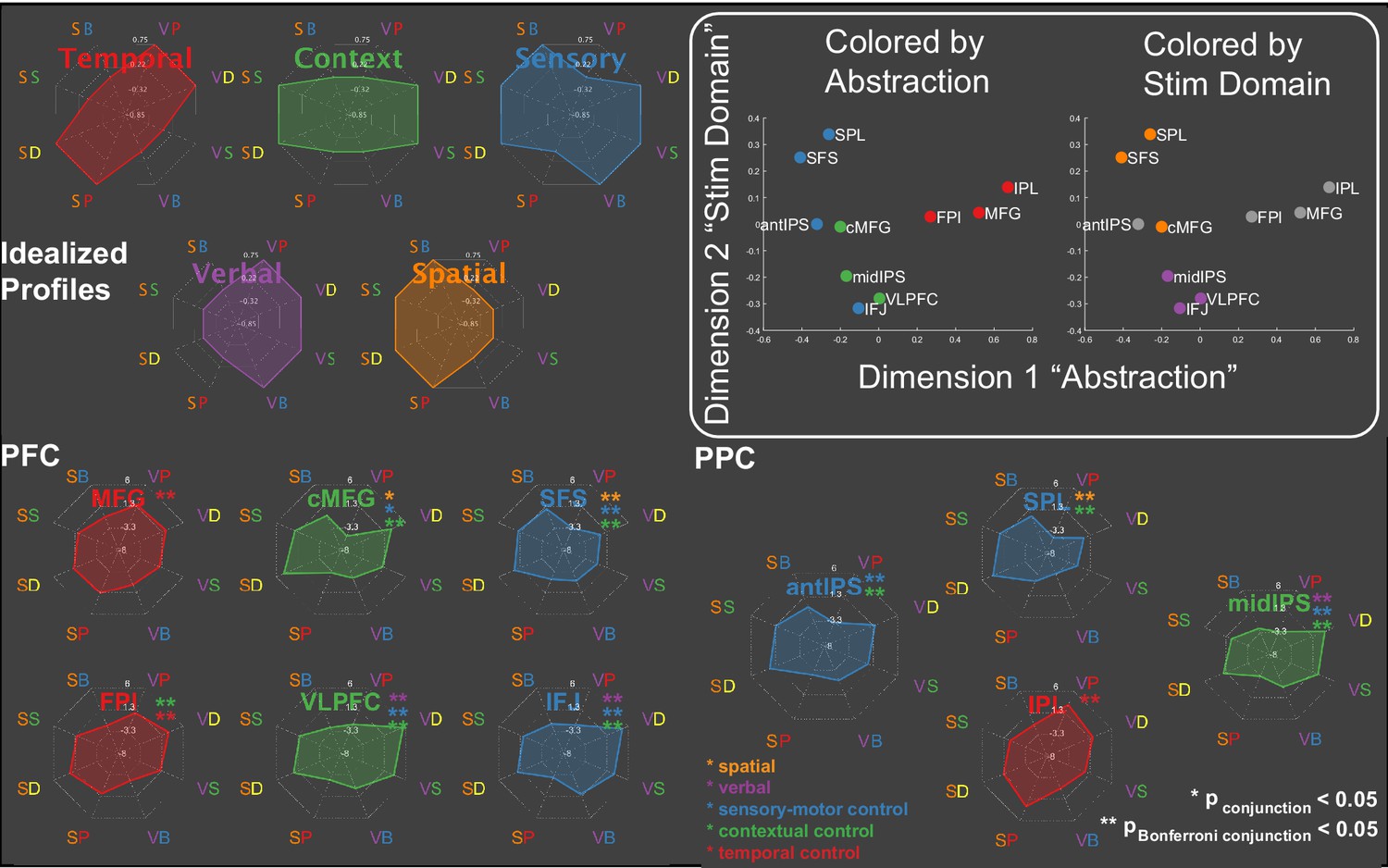
Activation profiles with reduced smoothing.
Details are identical to Figure 3.
Figure 4 with 1 supplement
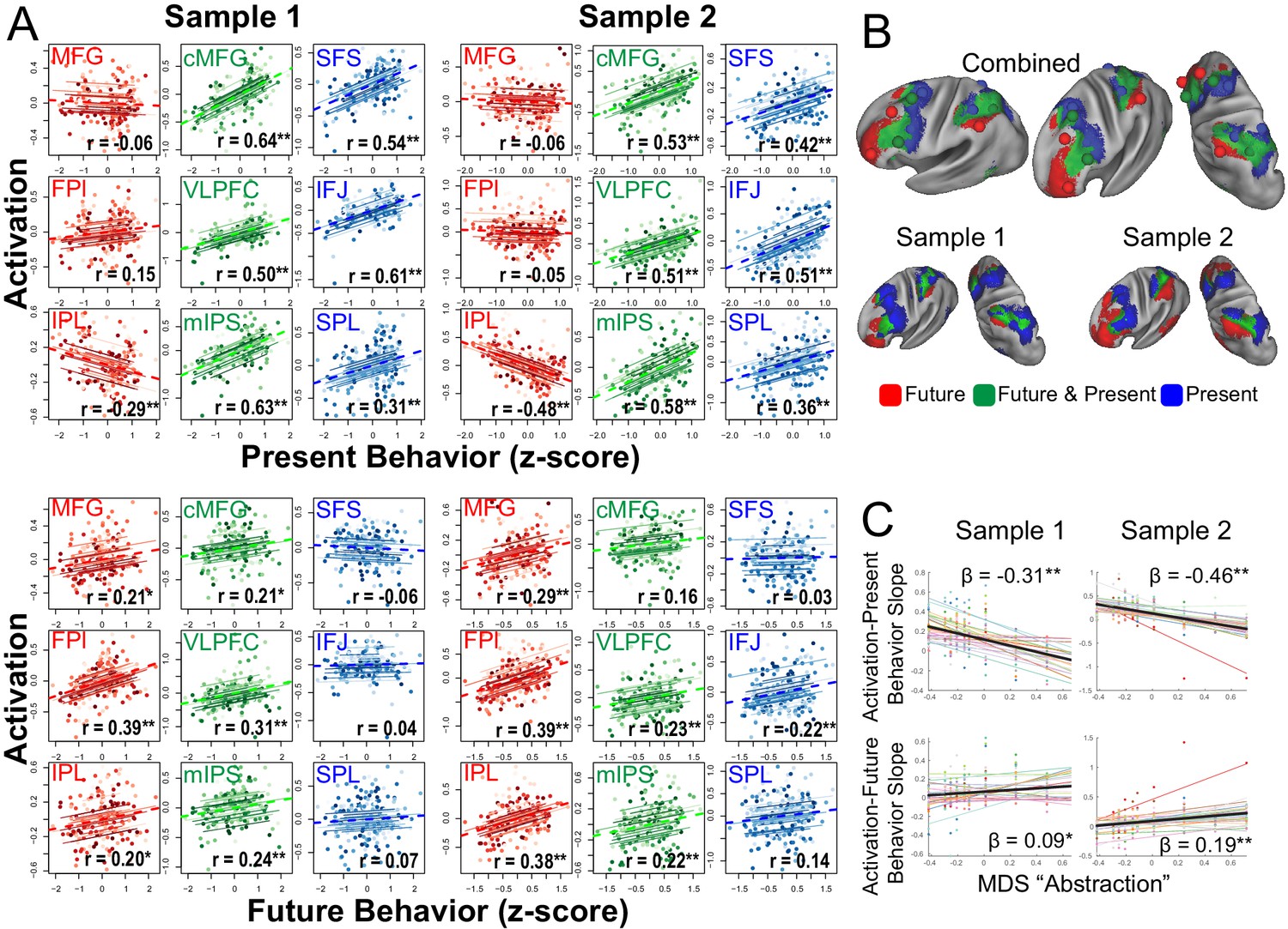
Brain-behavior relationships.
(A) Top: Repeated measures correlations between activation and present behavior (i.e. behavior during sub-task trials; see Figure 1). Areas related to sensory-motor control (blue) and contextual control (green) showed positive associations, while areas related to temporal control (red) showed no or negative associations. Bottom: Repeated measures correlations between activation and future behavior (i.e. behavior during return trials; see Figure 1). Areas related to temporal control (red) and contextual control (green) tended to show positive associations, while areas related to sensory-motor control (blue) tended to show no associations. ** indicates Bonferroni-corrected p<0.05. * indicates uncorrected p<0.05. (B) Voxel-wise partial correlations between activation and present behavior (blue), future behavior (red), and both (green). Results are visualized at p<0.001 with 124 voxel cluster extent. (C) Linear mixed effects modeling of the activation-present behavior slope (top) and activation-future behavior slope (bottom) using the first dimension of multi-dimensional scaling (MDS) depicted in Figure 3. * indicates p<0.05; ** indicates p<0.005.
Figure 4—figure supplement 1

Brain-behavior relationships with reduced smoothing.
Details are identical to Figure 4.
Figure 5 with 1 supplement
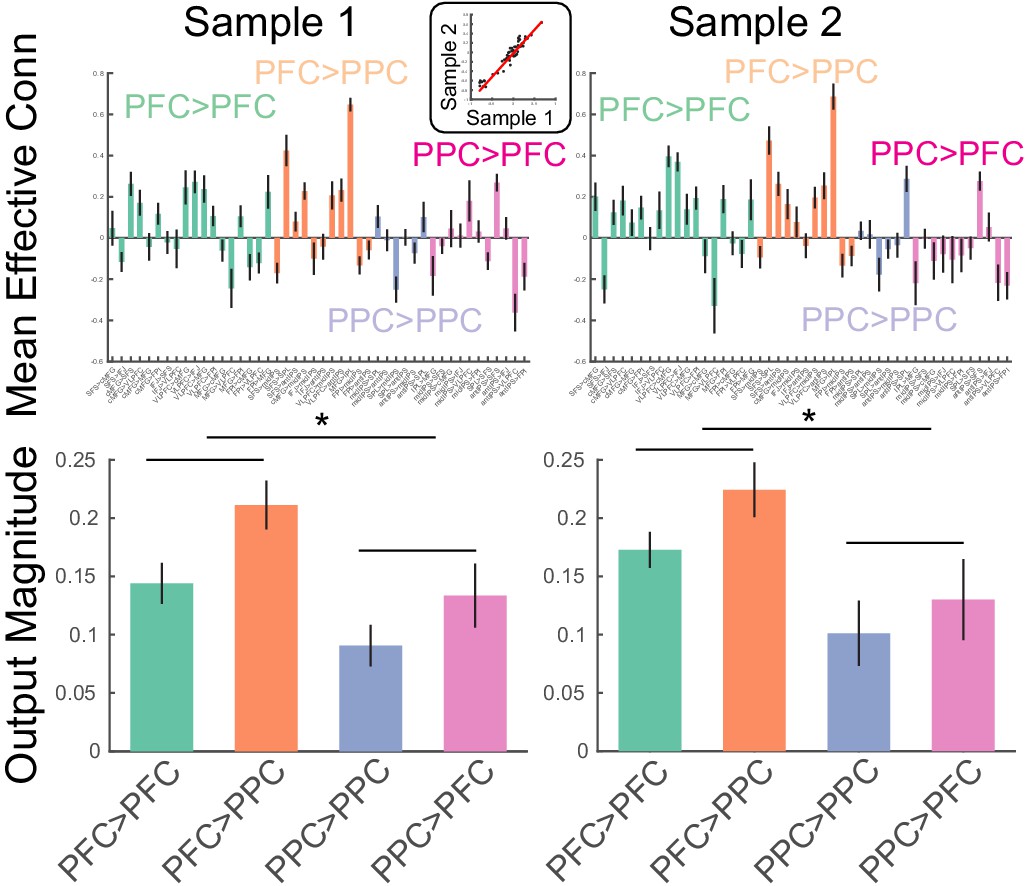
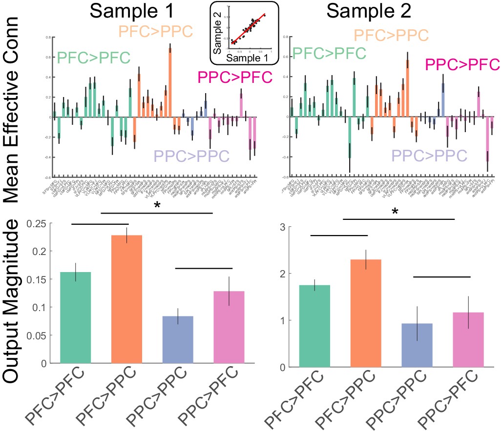
Estimates of static effective connectivity.
Bars are color coded by source>target lobe pairs. Top: estimates for each connection. Inset: correlation among sample averaged parameter estimates. Bottom: estimates averaged over source>target lobe pairs. Influences arising from the PFC were significantly stronger in magnitude than those arising from the PPC. * indicates p<0.05.
Figure 5—figure supplement 1
Estimates of static effective connectivity with reduced smoothing.
Details are identical to Figure 5.
Figure 6 with 2 supplements
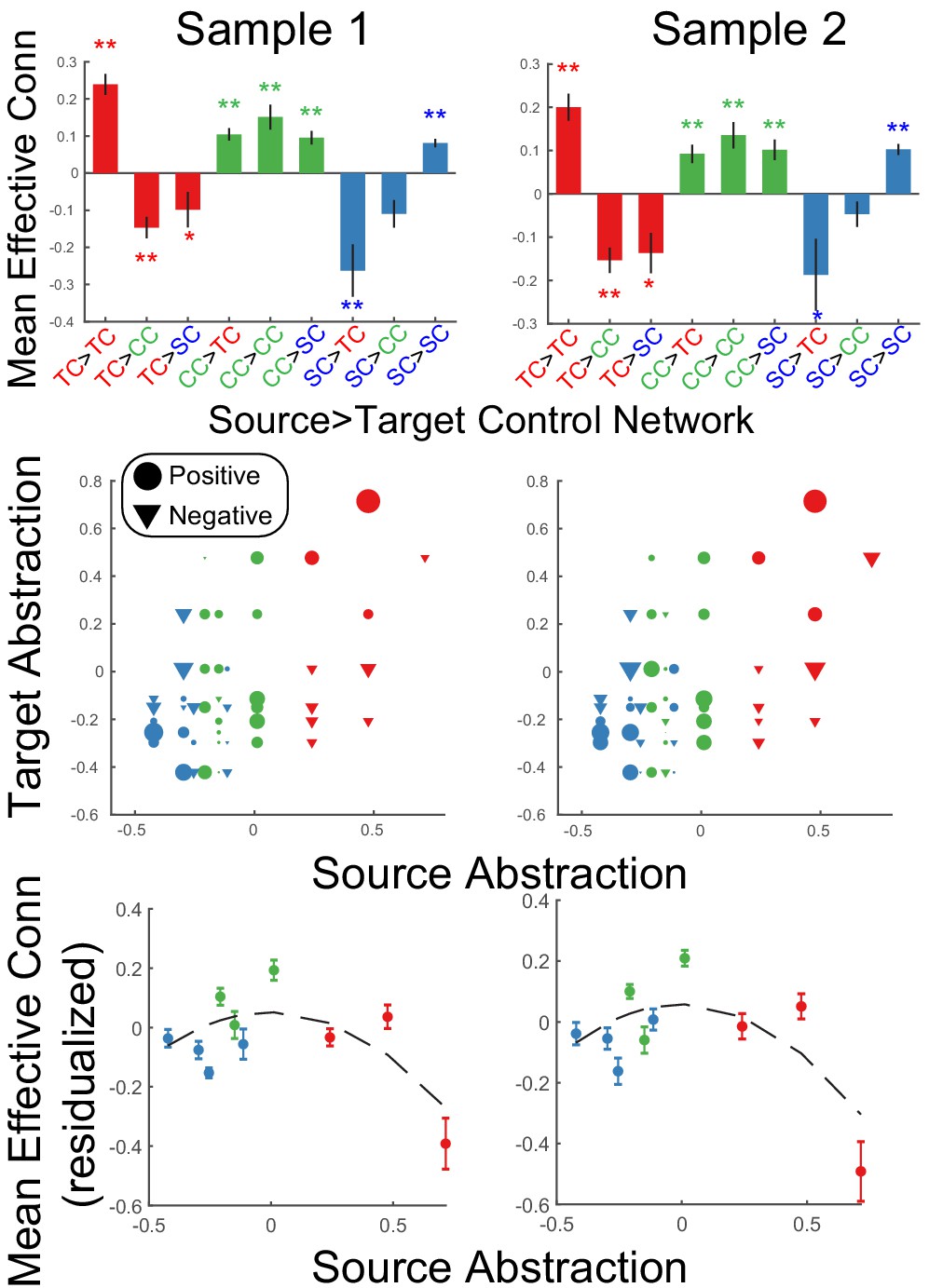
Static network interactions.
Top: Effective connectivity was averaged as a function of source>target network. Bars are colored as a function of the source network: TC – temporal control (red); CC – contextual control (green); SC – sensory-motor control (blue). ** denotes Bonferroni-corrected p<0.05. * denotes p<0.05 uncorrected. Middle: Effective connectivity organized by abstraction (first dimension of multi-dimensional scaling depicted in Figure 3). Circles denote positive interactions and inverted triangles denote negative interactions. Markers are scaled by the magnitude of effective connectivity. Markers are colored by the network assignments. Bottom: Data re-depicted to highlight the quadratic effect of source abstraction. Linear effects of target abstraction, source abstraction, and target x source abstraction have been regressed out to isolate the quadratic effect of source abstraction demonstrating that mean (positive) effective connectivity peaks at areas in the middle of the abstraction gradient.
Figure 6—figure supplement 1
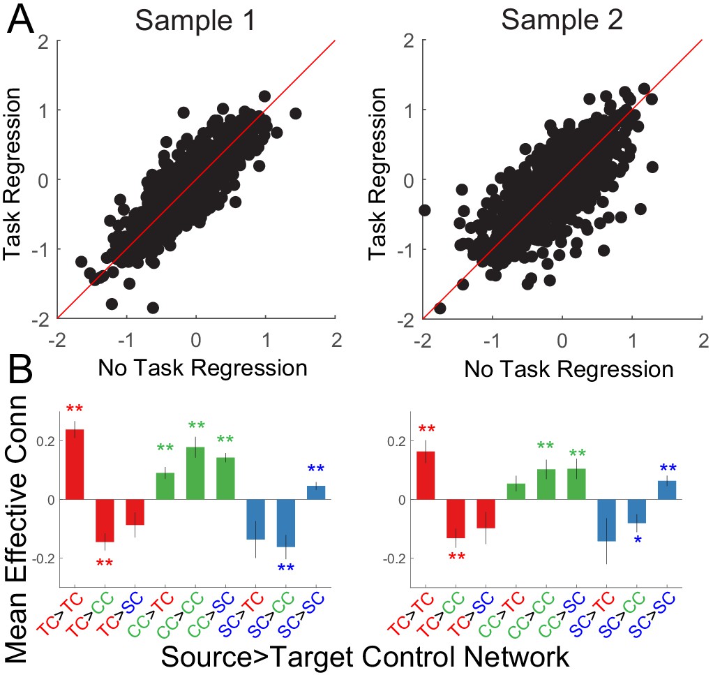
Effect of task signals on effective connectivity parameters and source x network interactions.
(A) Comparison of effective connectivity parameters with and without regressing out task signals. Bias (e.g. task-induced increases) would be apparent as a shift off of the diagonal (red line). No bias was observed. (B) Source x target network interactions after regressing out task signals. The same interaction was observed after regressing out task signals as was observed in the main text indicating that the interactions were not driven by task signals.
Figure 6—figure supplement 2
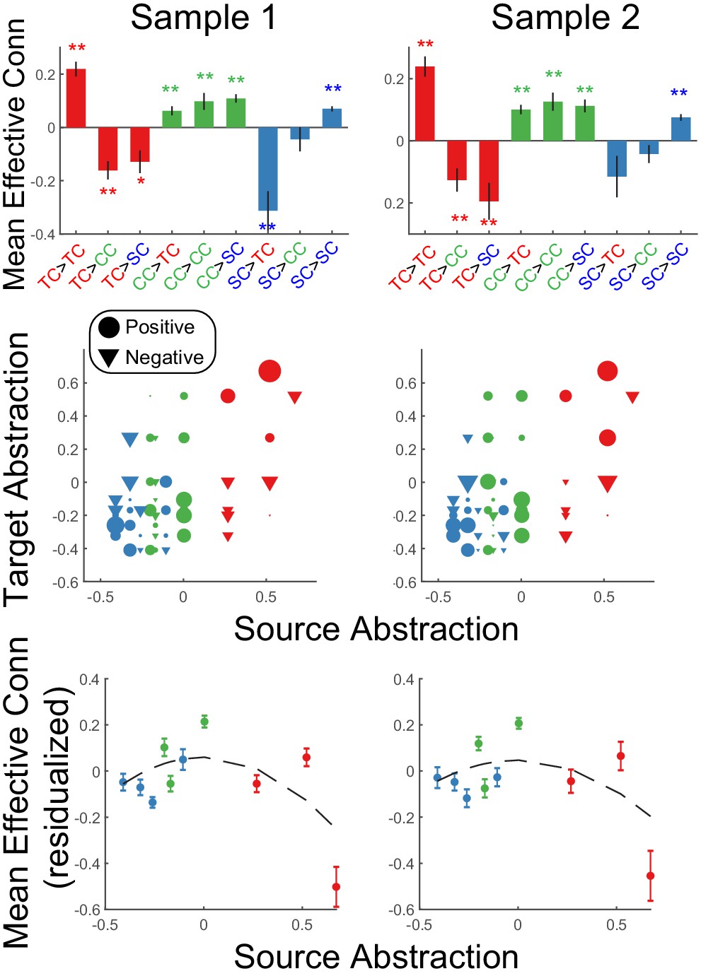
Static network interactions with reduced smoothing.
Details are identical to Figure 6.
Figure 7 with 3 supplements
Dynamic Interactions.
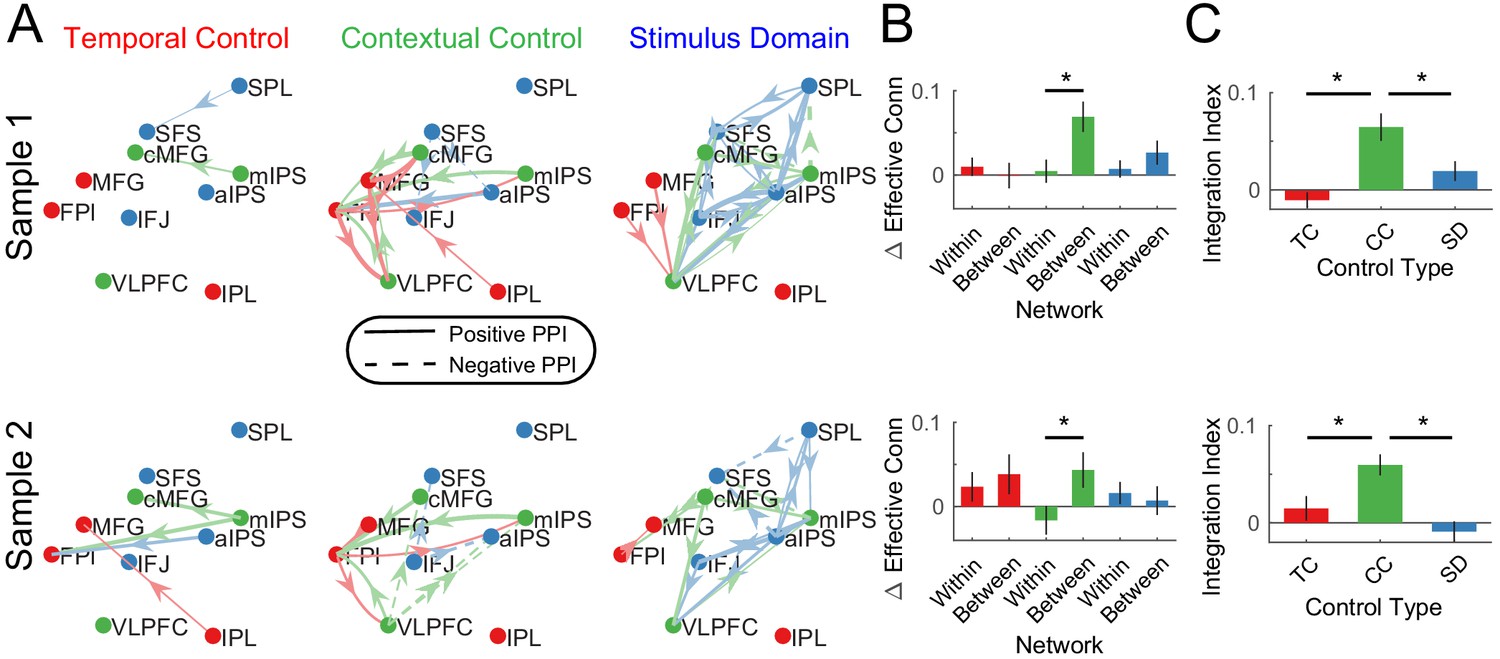
(A) Psychophysiological interactions (PPIs) for temporal control, contextual control, and stimulus domain contrasts. Solid lines indicate positive modulations of effective connectivity while dashed lines indicate negative modulations of effective connectivity. Arrows are colored by the network of the source node. Thickness of the arrows indicates the strength of modulations. Modulations are visualized at p<0.05 uncorrected. (B) Averaged within- and between-network modulations for the temporal control (red), contextual control (green), and stimulus domain (blue) contrasts. (C) Integration indices computed by contrasting between- minus within-network modulations for temporal control (TC), contextual control (CC), and stimulus domain (SD) contrasts.
Figure 7—figure supplement 1
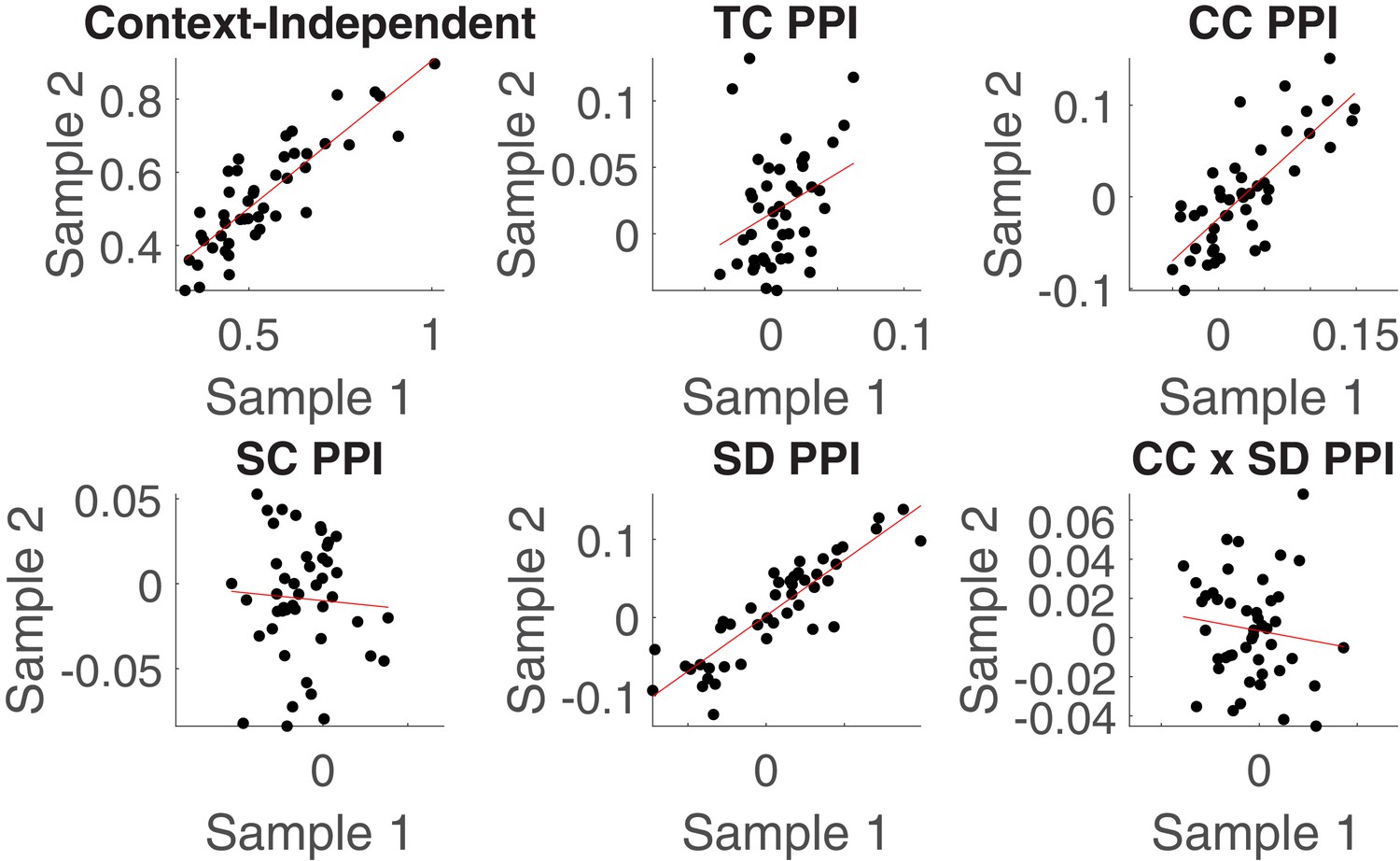
Sample averaged psychophysiological interaction (PPI) parameter estimates.
TC – temporal control; CC – contextual control; SC – sensory-motor control; SD – stimulus domain.
Figure 7—figure supplement 2
Comparison of the sensory-motor control contrast and stimulus domain contrasts.
Stimulus domain is jointly determined by verbal > spatial and spatial > verbal.
Figure 7—figure supplement 3

Dynamic interactions with reduced smoothing.
Details are identical to Figure 7.
Figure 8 with 3 supplements
Integration predicts higher level cognitive ability.
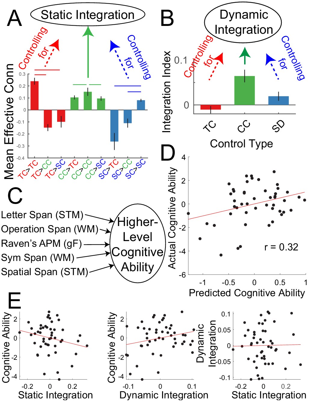
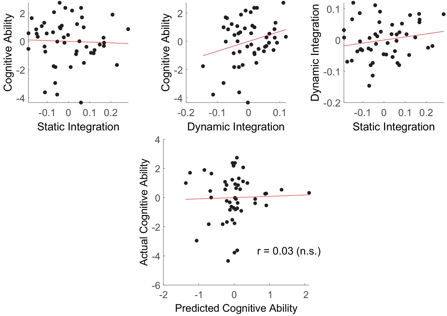
(A) Static integration was computed by contrasting between minus within-network effective connectivity of the contextual control network while controlling for (regressing out) the same contrast of the temporal control network and sensory-motor control network and individual differences in head motion. (B) Dynamic integration was based upon the integration index of the contextual control PPI’s while controlling for (regressing out) the integration indices of the temporal control and stimulus domain PPI’s and individual differences in head motion. (C) Higher level cognitive ability was computed as the first principle component of a battery of cognitive tests measuring capacity. (D) Cross-validated ridge regression was used to predict cognitive capacity based upon static and dynamic integration. The scatterplot depicts correlations between the predicted cognitive ability and actual cognitive ability. (E) Correlations among static integration, dynamic integration, and cognitive ability.
Figure 8—figure supplement 1
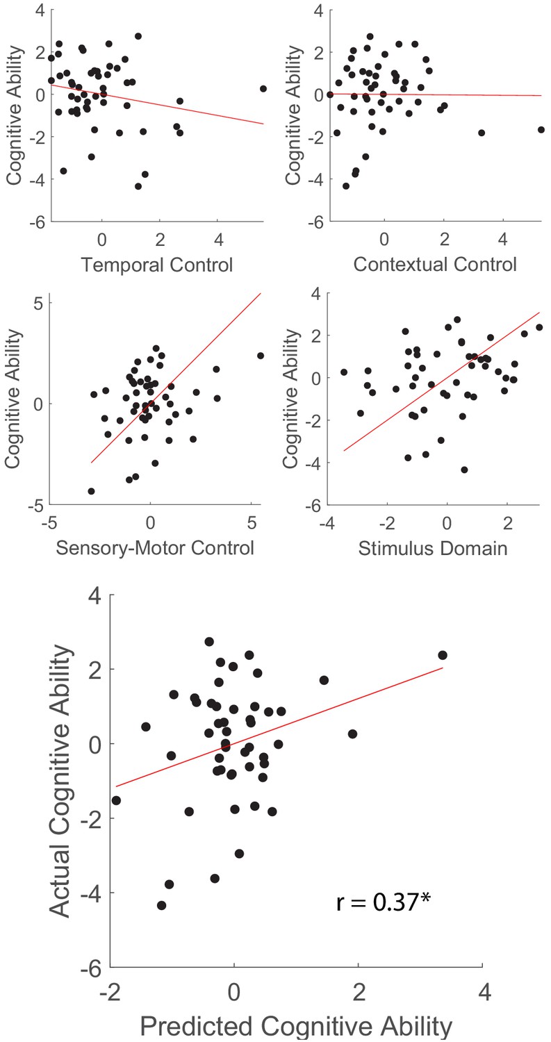
Activations predict higher level cognitive ability.
Cognitive control and stimulus domain related activations were used as features to predict cognitive ability in a similar manner to the use of integration measures to predict cognitive ability. Principle components analysis was used to create factors associated with temporal control (temporal control contrast activations in FPl, MFG, and IPL), contextual control (contextual control contrast activations in VLPFC, cMFG, and midIPS), sensory-motor control (sensory-motor control contrast activations in IFJ, SFS, antIPS, and SPL), and stimulus domain (stimulus domain contrast activations in IFJ, SFS, antIPS, and SPL). Note that all contrasts are orthogonal to one another. Cross-validated ridge regression was used to predict cognitive ability based upon the activation measures.
Figure 8—figure supplement 2
Integration does not predict higher-level cognitive ability with reduced smoothing.
Details are identical to Figure 8D–E.
Figure 8—figure supplement 3
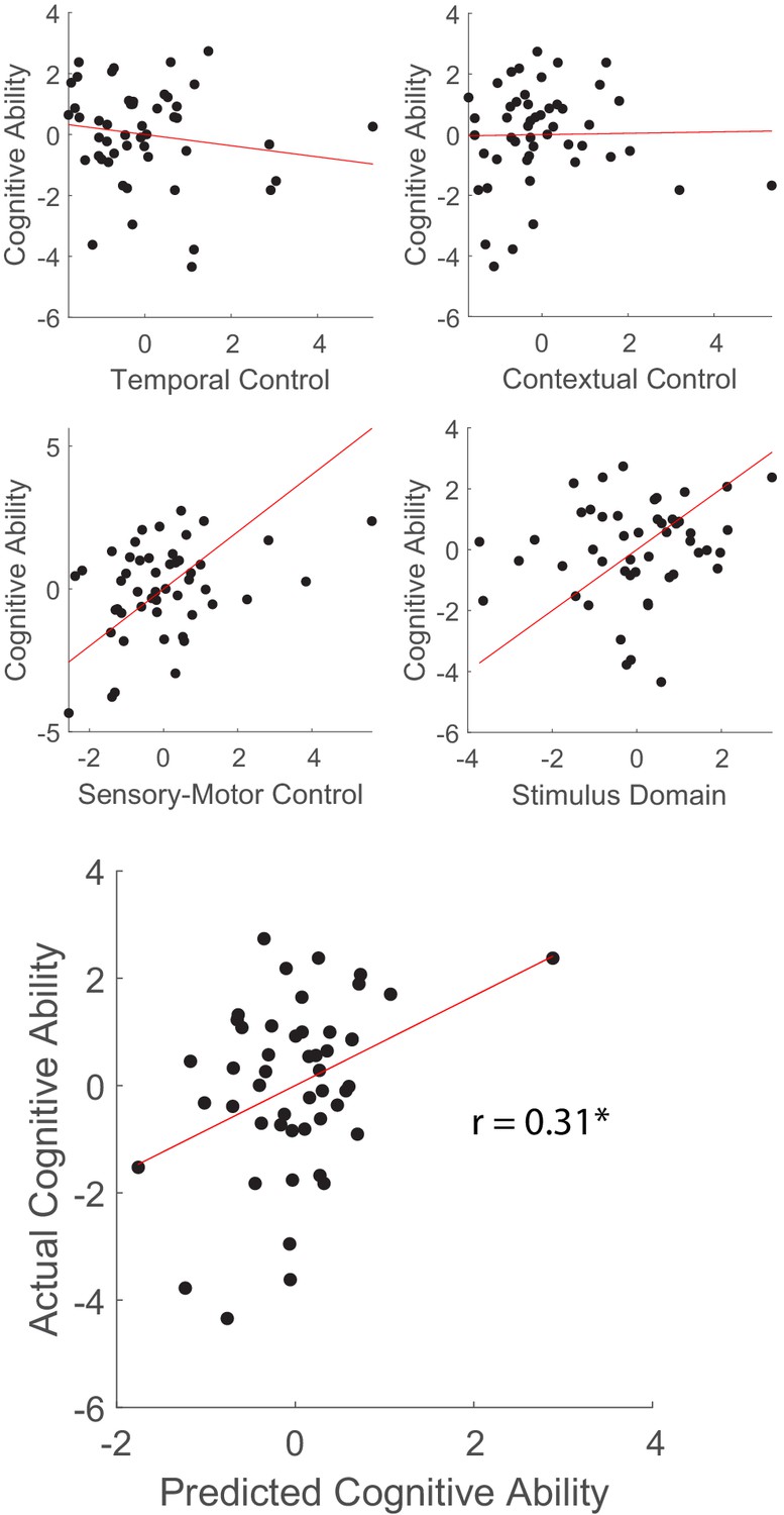
With reduced smoothing, activation-based measures remain significantly predictive of higher-level cognitive ability.
Figure 9 with 4 supplements
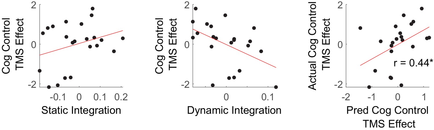
Integration predicts transcranial magnetic stimulation (TMS) effects.
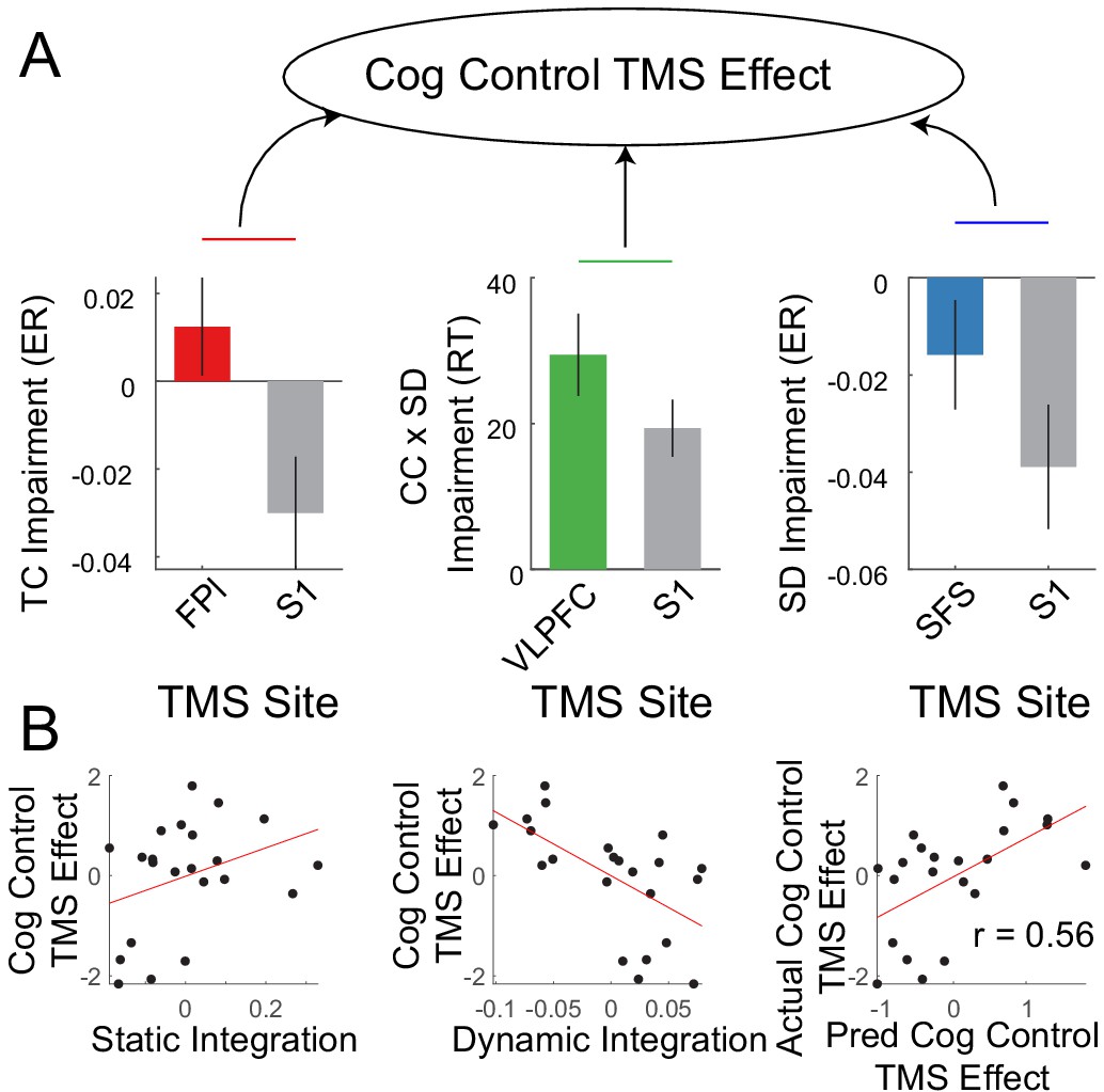
(A) Previously reportedNee and D'Esposito, 2017 cognitive control impairments induced by continuous theta-burst TMS were combined using principle components analysis to derive a general susceptibility to PFC TMS. (B) Correlations between cognitive control TMS effects and static and dynamic integration. Leave-one-out cross-validated ridge regression was used to predict TMS effects using static and dynamic integration. Scatterplot depicts the correlation between predicted and actual TMS impairments.
Figure 9—figure supplement 1
Integration predicts transcranial magnetic stimulation (TMS) effects with reduced smoothing.
Details are identical to Figure 9B.
Figure 9—figure supplement 2

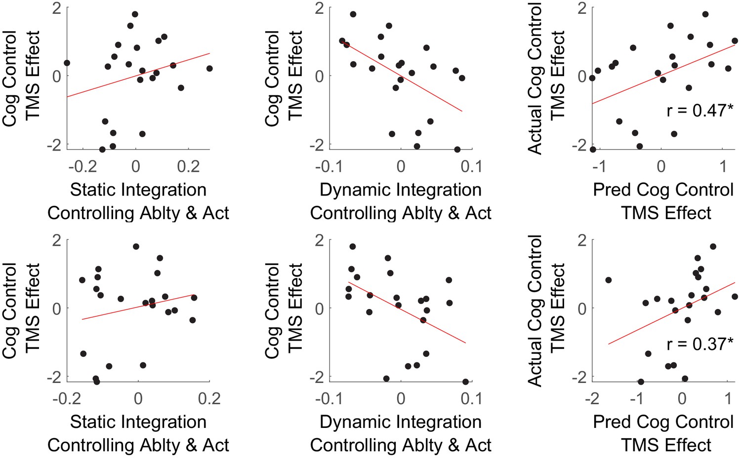
Integration predicts transcranial magnetic stimulation (TMS) effects after controlling for cognitive ability.
Details are the same as Figure 9 except that cognitive ability has been regressed out of static and dynamic integration measures. Top: standard (8 mm smoothing). Bottom: reduced (4 mm smoothing).
Figure 9—figure supplement 3
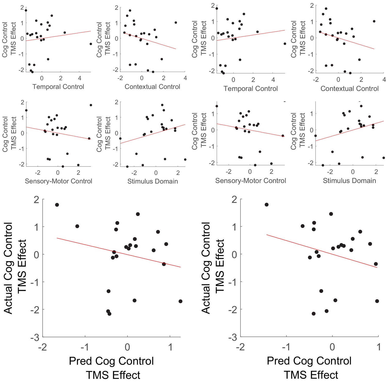
Activations do not predict TMS effects.
Cognitive control and stimulus domain related activations were used as features to predict TMS effects in a similar manner to the use of integration measures to predict TMS effects. Principle components analysis was used to create factors associated with temporal control (temporal control contrast activations in FPl, MFG, and IPL), contextual control (contextual control contrast activations in VLPFC, cMFG, and midIPS), sensory-motor control (sensory-motor control contrast activations in IFJ, SFS, antIPS, and SPL), and stimulus domain (stimulus domain contrast activations in IFJ, SFS, antIPS, and SPL). Note that all contrasts are orthogonal to one another. Cross-validated ridge regression was used to predict TMS effects based upon the activation measures. Note in both cases, predicted and actual TMS effects were negatively correlated indicating that activation measures are not useful for predicting TMS effects. Left: standard (8 mm smoothing). Right: reduced (4 mm smoothing).
Figure 9—figure supplement 4
Integration predicts transcranial magnetic stimulation (TMS) effects after controlling for both cognitive ability and activations.
Details are the same as Figure 9 except that cognitive ability and activations have been regressed out of static and dynamic integration measures. Top: standard (8 mm smoothing). Bottom: reduced (4 mm smoothing).
Tables
Table 1
Coordinates of regions-of-interest reported in MNI space.
FPl – lateral frontal pole; MFG – middle frontal gyrus; VLPFC – ventrolateral prefrontal cortex; cMFG – caudal middle frontal gyrus; IFJ – inferior frontal junction; SFS – superior frontal sulcus; IPL – inferior parietal lobule; mIPS – mid intra-parietal sulcus; aIPS – anterior intra-parietal sulcus; SPL – superior parietal lobule.
| Sample 1 | Sample 2 | |||||
|---|---|---|---|---|---|---|
| Area | X | Y | Z | X | Y | Z |
| FPl | −44 | 48 | 4 | −36 | 52 | 0 |
| MFG | −38 | 28 | 44 | −36 | 34 | 38 |
| VLPFC | −52 | 20 | 28 | −42 | 30 | 20 |
| cMFG | −34 | 10 | 60 | −30 | 6 | 56 |
| IFJ | −38 | 6 | 26 | −42 | 10 | 24 |
| SFS | −22 | 0 | 54 | −20 | 0 | 56 |
| IPL | −54 | −50 | 44 | −56 | −52 | 42 |
| mIPS | −28 | −60 | 42 | −26 | −56 | 44 |
| aIPS | −34 | −40 | 46 | −30 | −42 | 42 |
| SPL | −14 | −52 | 64 | −12 | −60 | 58 |
Additional files
-
Supplementary file 1
Tables containing supplemental behavioral analyses.
Factorial ANOVA’s for the sub-task trials and return trials. RT – reaction time; ACC – accuracy; ME – main effect.
- https://cdn.elifesciences.org/articles/57244/elife-57244-supp1-v2.docx
-
Transparent reporting form
- https://cdn.elifesciences.org/articles/57244/elife-57244-transrepform-v2.docx
Download links
A two-part list of links to download the article, or parts of the article, in various formats.
Downloads (link to download the article as PDF)
Open citations (links to open the citations from this article in various online reference manager services)
Cite this article (links to download the citations from this article in formats compatible with various reference manager tools)
Integrative frontal-parietal dynamics supporting cognitive control
eLife 10:e57244.
https://doi.org/10.7554/eLife.57244


