Curvature domains in V4 of macaque monkey
- Department of Neurology of the Second Affiliated Hospital, Interdisciplinary Institute of Neuroscience and Technology, School of Medicine, Zhejiang University, China
- Key Laboratory for Biomedical Engineering, of Ministry of Education, Zhejiang University, China
- Division of Neuroscience, Oregon National Primate Research Center, Oregon Health & Science University, United States
Figures
Figure 1
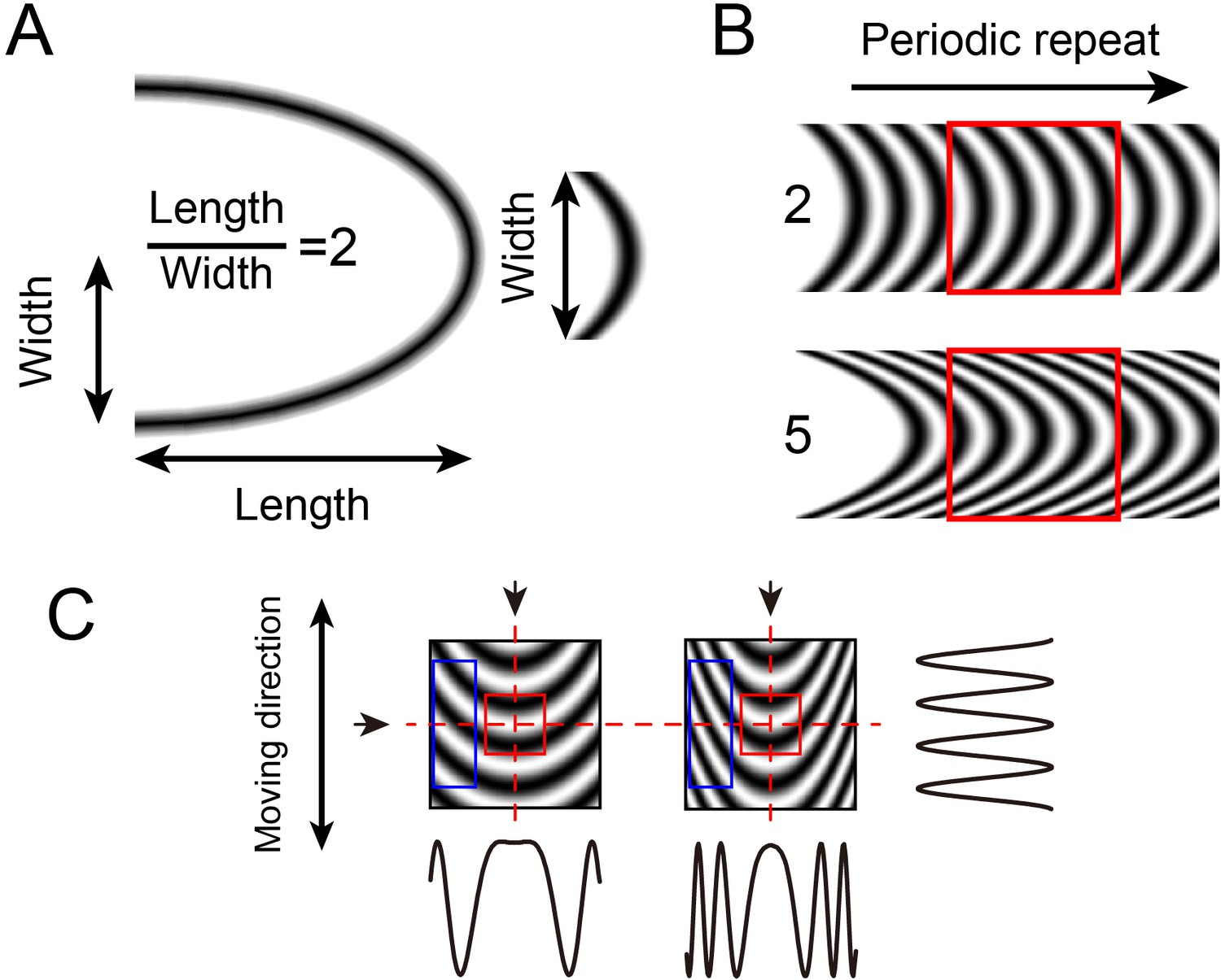
Curvature grating stimuli.
(A) Calculation of curvature index. Width is half of the ellipse width. (B) Constructing curvature grating by periodic repeat. One low (index = 2) and one high (index = 5) curvature grating shown. (C) Luminance profiles of different stimuli in different directions. The profiles at the vertical axis (arrows at top, profile at right) of the two stimuli are similar, but differ in the horizontal axis (arrow at left, profiles below). The higher the curvature degree, the higher the spatial frequency towards the edge of the stimulus. Red square: central region, blue rectangle: flanking regions.
Figure 2 with 13 supplements
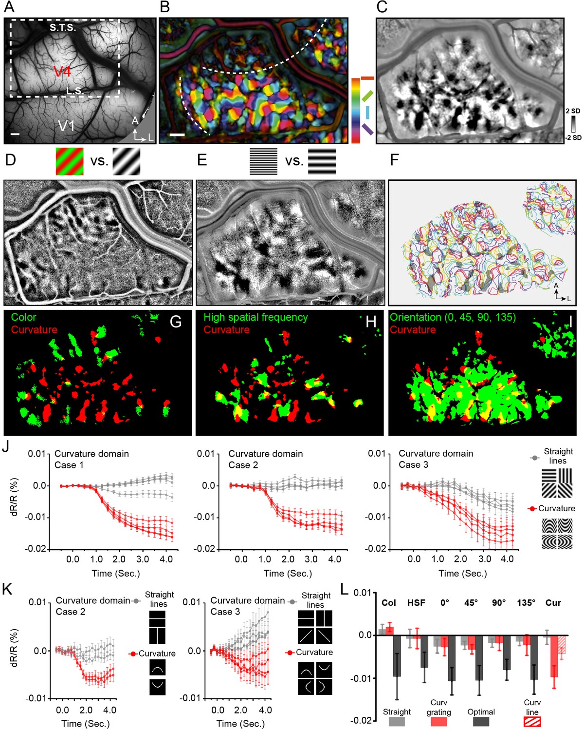
Curvature domains exist and are distinct.
(A) View of cortical surface in Case 1. Dotted box: region shown in B-I. L.S., lunate sulcus. S.T.S., superior temporal sulcus, A, anterior, L, lateral. B-I: Case 1. (B) Color-coded orientation preference map. White dashed lines: approximate borders between color and orientation bands. (C) Curvature map: all curved minus all straight gratings. (D) Color preference map. (E) High spatial frequency preference map (4 cycle/deg vs. 0.5 cycle/deg). (F) Curvature domains (gray patches, two-tailed t-test, p<0.01) superimposed on iso-orientation contours. (G-I) Overlay of curvature domains (red) and G: color domains (green, from D), H: high spatial frequency domains (green, from E), I: all orientation domains (green). (J) Response time courses of curvature domains from Case 1 (left), Case 2 (middle), and Case 3 (right). Red lines: preferred stimuli. Gray lines: non-preferred stimuli. (K) Response time courses of curvature domains to flashed curved lines. Red timecourses: flashed curved lines. Gray timecourses: flashed straight lines. (L) Summary of response amplitudes for color (Col), high spatial frequency (HSF), orientation (0°, 45°, 90°, 135°), and curvature (Cur) domains shown in J, K. Gray: straight grating. Red: Curved grating. Black: optimal stimulus responses (except for Cur). For Cur, optimal response was to curved gratings (red) and to flashed curved lines (hatched red). Scale bar: 1 mm. Error bars: SEM (timecourses in J, K), SD (histogram in L).
Figure 2—figure supplement 1
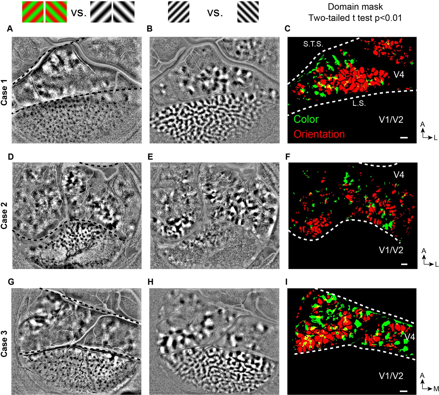
Large field of view of functional maps in Cases 1–3.
Color (left column) and orientation (middle column) maps in V1, V2, and V4. Third column: overlay of color preferring (green) and orientation selective pixels (red). White dotted lines: lunate sulcus (LS) and superior temporal sulcus (STS). For all maps, the locations of functional domains were determined by t-value maps (t-map, two-tailed t test, p<0.01) which were calculated by comparing, pixel by pixel, the responses between two different conditions (A: color vs. achromatic, B: 45° vs. 135°). Case 2: some of cortex in V1 was out of focus in initial session. Map obtained from another session shows clear color and orientation maps in V1. Scale bar: 1 mm.
Figure 2—figure supplement 2

V1/V2 and V4 represent different retinotopic locations in the same field of view.
Case 1 (A–F), Case 2 (G–L), Case 3 (M). A, G. The center of the 4 deg curvature grating (1 deg size red square in A, G) is centered on the field of view in V4 [red oval in B (flashed line at x = 0), H, M (flashed 1 deg square)], as determined by the mapping of vertical (C, I) and horizontal (D, J) dotted lines (shown in A, G) [note the lack of V1 activation]. The region of V1 visible within the same field of view (posterior to lunate) represents a different retinotopic location (green square in A, G; green oval in B, H), as determined by the mapping of vertical (E, K) and horizontal (F, L) dotted lines (shown in A, G). Thus, it was not possible to image the response to the central curvature stimulus in both V1 and V4 simultaneously. Dotted line (line width: 0.2 degrees. Drift direction: along the line) for retinotopic mapping. Xn, Yn: dotted line position (in n degrees) over center of curvature stimulus. M. Retinotopic mapping example from Case 3. For subdomain analysis, we focused on the regions outlined by these red dashed ovals (corresponding to the central 1 deg region).
Figure 2—figure supplement 3
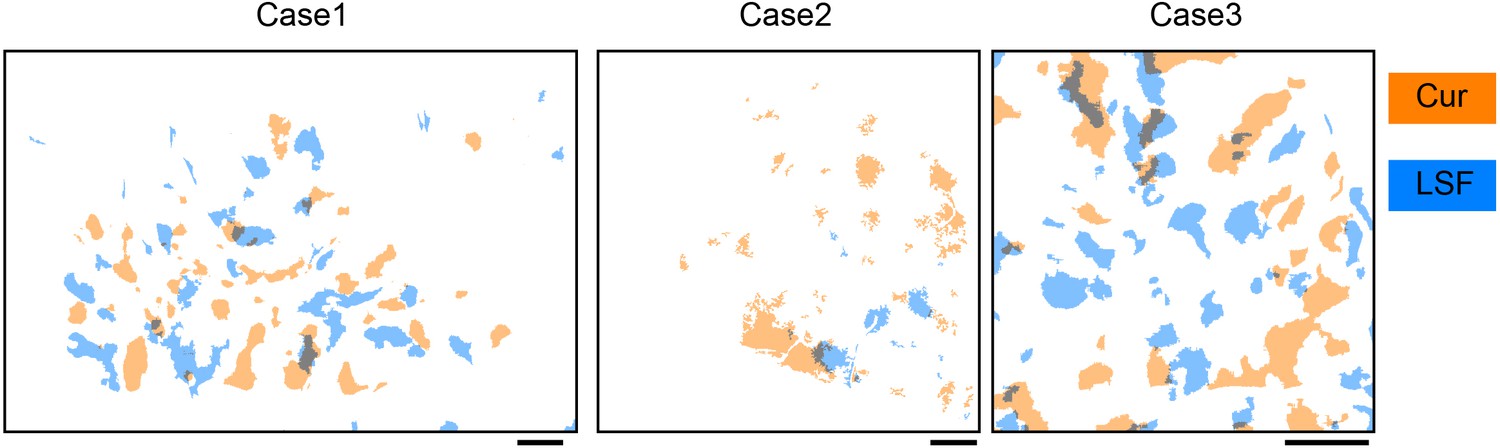
Relationship between curvature domain and low SF domain.
Based on our results, curvature domains and low SF domains are largely separated (curvature domain: orange region; low SF domain: blue region).
Figure 2—figure supplement 4
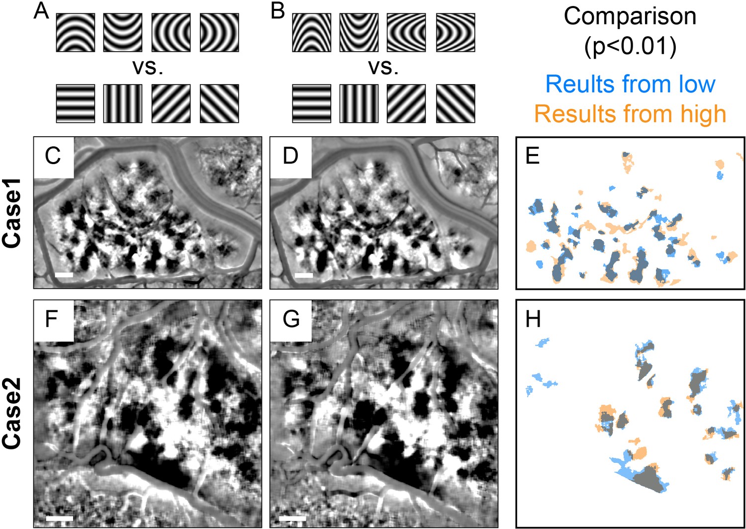
Low and high curvature maps are highly overlapped (two Cases across two sessions).
Maps of low vs. high curvature. (A-B) Stimuli with low (A, Length/width = 2) vs. high (B, Length/width = 5) curvature degrees. These are compared with straight orientation gratings of the same SF. C-G: subtracted curvature maps for Case 1 (C,F) and Case 2 (D,G). (E, H) Overlay of low vs. high T maps (p<0.01). Blue: low SF. Orange: high SF. Scale bar: 1 mm.
Figure 2—figure supplement 5

Stability of curvature response across different days.
Maps of all curvature minus all straight. A and B (Case 1), and C and D (Case 2) imaged on different days. Red dots: corresponding curvature domains imaged on different days. Scale bar: 1 mm.
Figure 2—figure supplement 6

Imaging of curvature responses and scrambled map in the same cortical region (from Case 3).
(A) Scrambled version of a curvature grating created by dividing the grating (each frame) into 64 subunits and rearranging the subunits randomly. (B) Curvature map (curvature vs. straight). (C) Scrambled map (Scrambled vs. Straight, The scrambled stimuli consist of patterns of scrambled patches whose elements are randomly changing frame by frame across time). Scale bar: 1 mm.
Figure 2—figure supplement 7
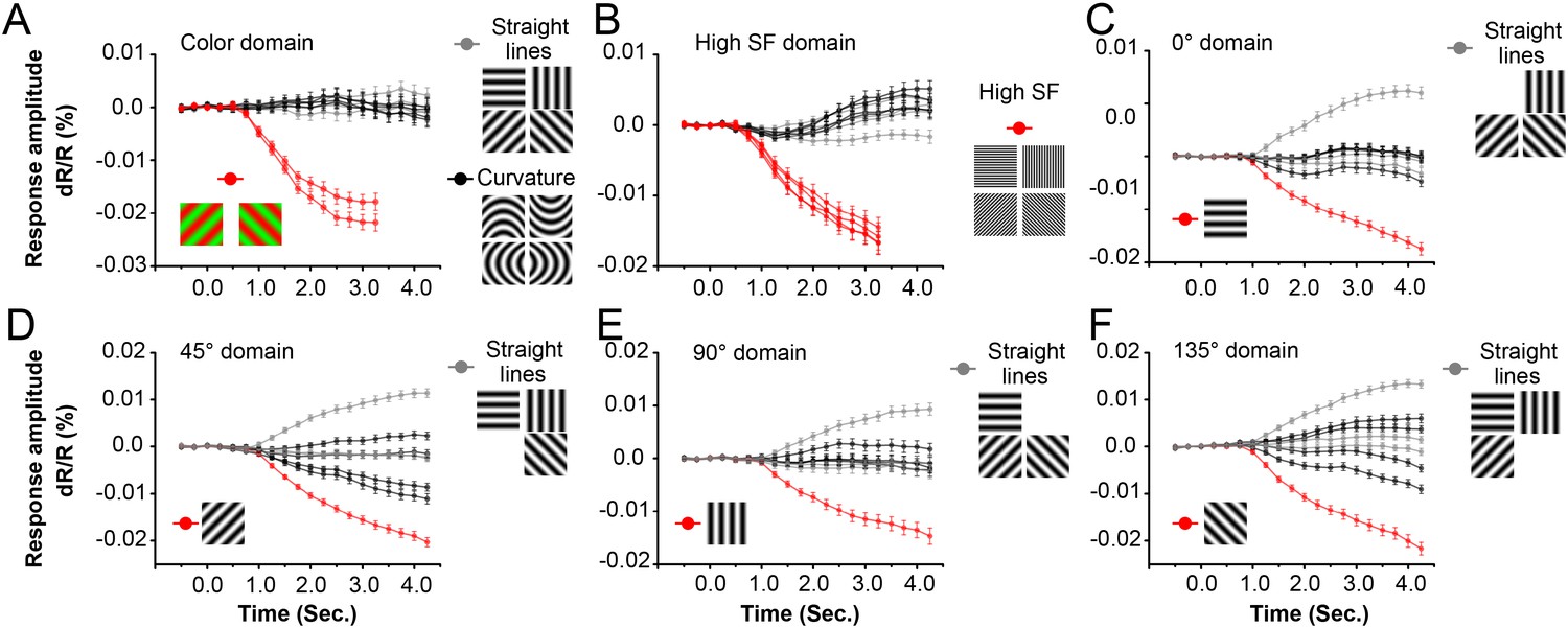
Supporting graphs for Figure 2L.
Red lines: preferred stimuli for each domain type. Gray lines, black lines: non-preferred stimuli (see insets next to each graph). (A) Color domains exhibit robust response to isoluminant color gratings (red line) but weak response to achromatic gratings (gray lines: straight gratings, black lines: curved gratings). (B) High spatial frequency domains responded strongly to achromatic gratings of high spatial frequency (red lines) but poorly to low spatial frequency gratings (either straight, gray lines, or curved, black lines). Note that, both color domains and high spatial frequency domains exhibited poor responses to curvature stimuli. (color mean dR/R = 6.8 × 10⁻⁶; HSF mean dR/R = 1.5 × 10⁻⁶). (C-F) Orientation domains (0°, 45°, 90°, 135°) exhibited strongest response to gratings of their respective optimal orientations (red line), relative suppression to gratings of orthogonal orientation (top gray line), and weak responses to other straight orientations (other gray lines). In comparison, they displayed relatively little response to curved gratings (black lines) (Wilcoxon test, p<10−5 for each of the four optimal orientation responses compared to response to all four curvatures summed).
Figure 2—figure supplement 8
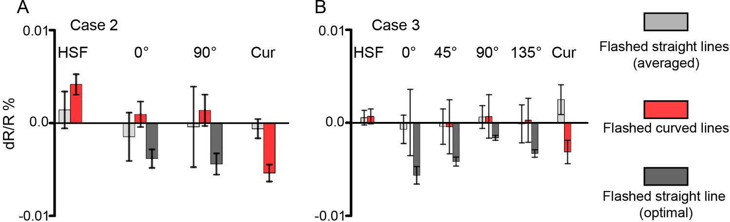
Straight orientation domains and high spatial frequency domains exhibit weak responses to single curved lines.
Peak responses for high spatial frequency (HSF), orientation (Case 2: 0°, 90°; Case3: 0°, 45°, 90°, 135°), and curvature (Cur) domains in Case 2 (A) and Case 3 (B) to flashed lines. Light gray: straight lines. Red: curved lines. Gray: Optimal straight lines. Error bars: SD.
Figure 2—figure supplement 9
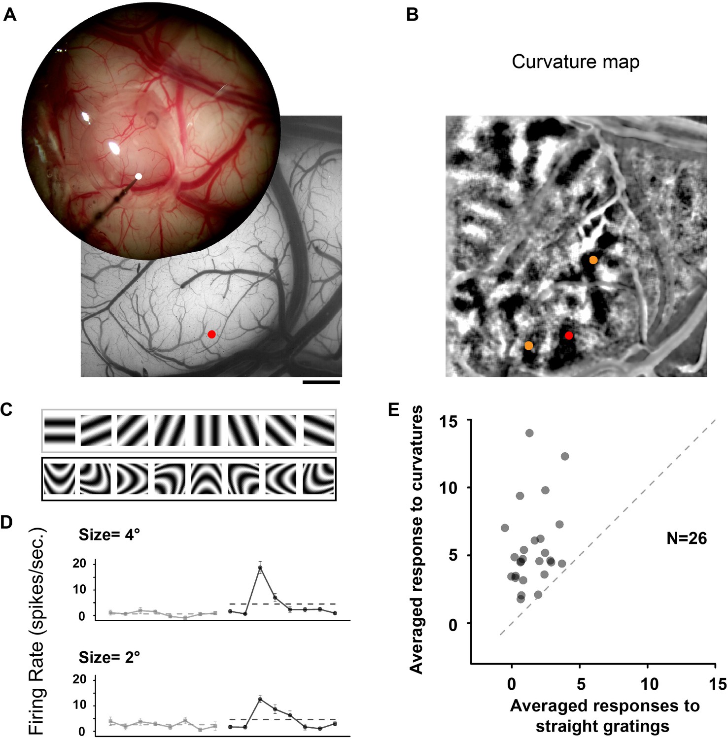
Neurons in curvature domains prefer curvature.
(A) A single electrode targeting a curvature domain in V4 (Case 3). (B) Positions of all three penetrations on the curvature map (all curve minus all straight). (C) Straight stimuli and curved stimuli used for straight and curvature orientation tuning. (D) Straight (light gray) and Curvature (dark gray) orientation tuning of a single unit. This neuron exhibited strong responses to one particular curvature orientation. The stimulus size (upper: 4 degrees, lower: 2 degrees) does not affect the tuning profile. Dashed lines: average firing rates to straight gratings (gray) and curved gratings (black). (E) Comparison between averaged responses to curvature and to straight gratings. 26 units (19 single units and 7 multi-units from three penetrations in three experimental sessions. For 14 units, the stimulus sizes are 3 degrees; for the other 12 units, the stimulus sizes are 4 degrees). On average, these neurons prefer curvature to straight stimuli.
Figure 2—figure supplement 10
Curvature domains were not observed in V1.
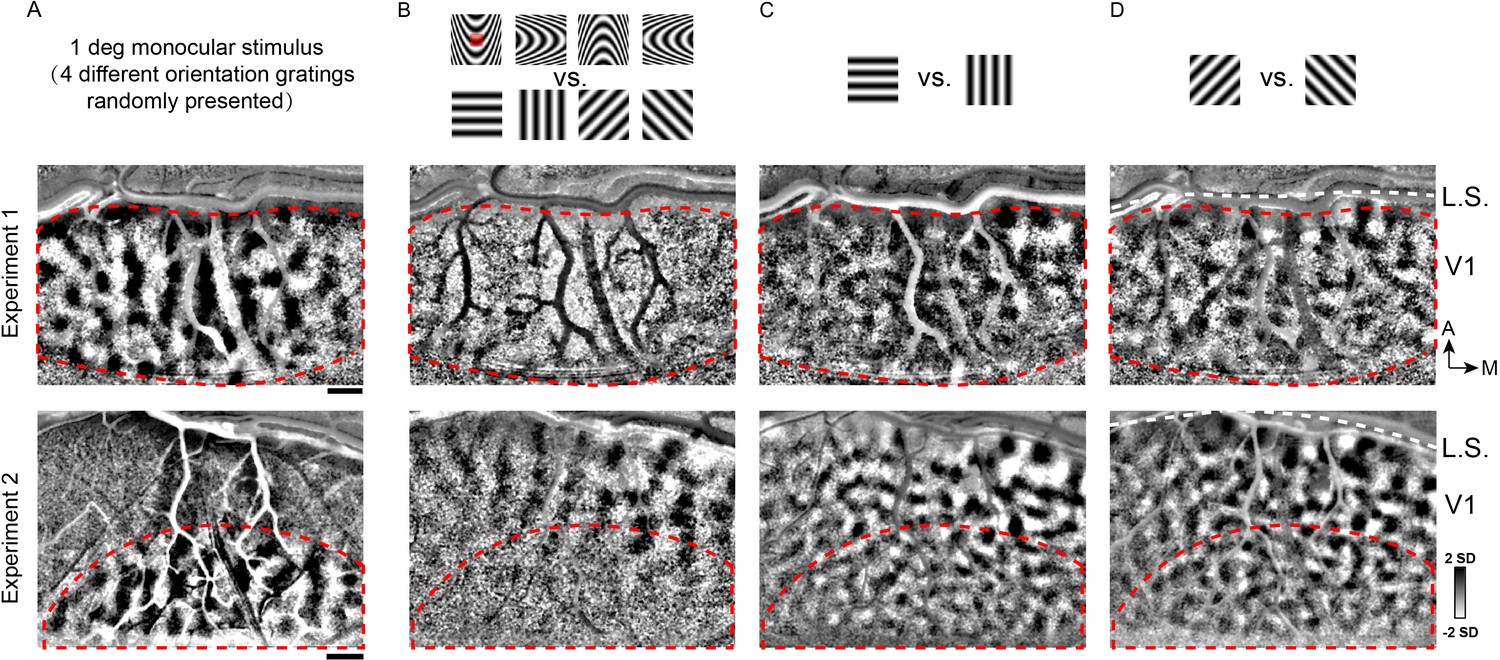
Field of view over V1. (A) Ocular dominance columns acquired by presenting monocular oriented stimuli one degree in size (by summing responses across four orientations). Red dashed line: activated V1 region. (B) Cortical response comparison between curved and straight stimuli (stimulus size: four degrees, from the same experiment session). These stimuli shared the same center locations as shown in A. Within the central 1 deg region (within red dashed line, corresponding to location of central red square), there was no obvious preference or response pattern for curvature over straight. Differences only appeared in response to the flanks of the stimulus (outside the red dotted line), perhaps due to different spatial frequencies between flanking regions of the straight and curvature stimuli. (C, D) Orientation maps acquired with the straight stimuli in B. White dotted lines: lunate sulcus (L.S.).
Figure 2—figure supplement 11
Very little V2 is available on surface.
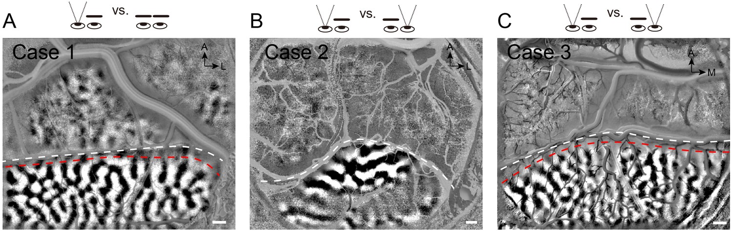
Location of V1/V2 border revealed by ocular dominance mapping (three cases). White dashed line: lunate sulcus. Red dashed line: V1/V2 border.
Figure 2—figure supplement 12
Curvature domains are not pinwheel centers.
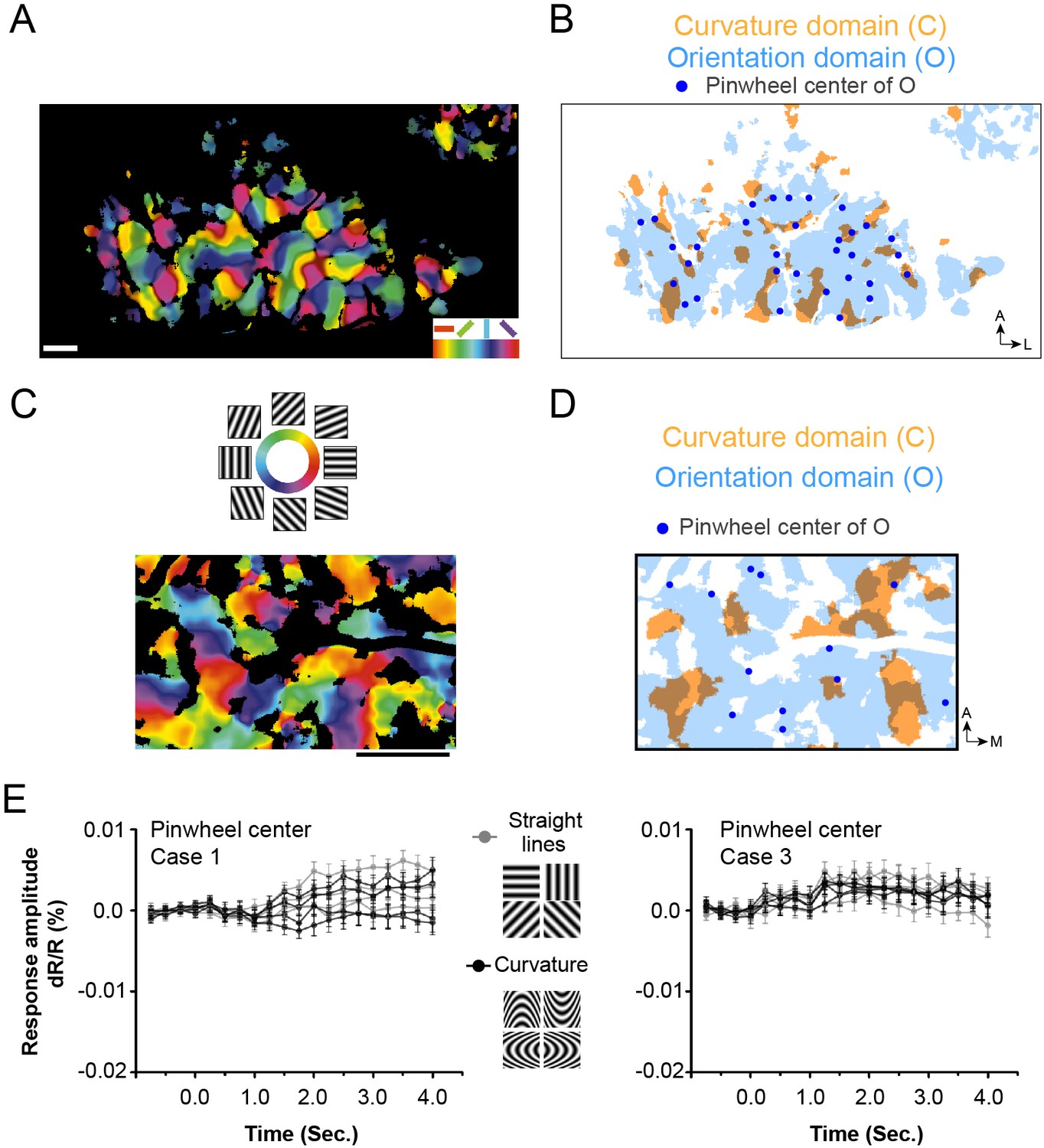
(A-B: Case 1, C-D: Case 3). (A, C) Orientation map from two cases (A: Case 1, C: Case 3). Different colors represent different orientation preferences. Only the pixels that can distinguished two orthogonal orientations (responses comparison between two orthogonal conditions, two tailed t test, p<0.01) and show significant responses (compared with blank condition, two tailed t test, p<0.01) were kept. (B, D). Locations of curvature domains (orange) and orientation domains (blue). Blue dots: pinwheel centers of orientation domains. Most of the curvature domains are not close to orientation pinwheel centers. (E) Response timecourse of pinwheel centers from these two cases. Gray lines: responses to straight gratings (four orientations). Black lines: responses to curvatures (four orientations).
Figure 2—figure supplement 13
Curvature domains can not be fully explained by end-stopping.
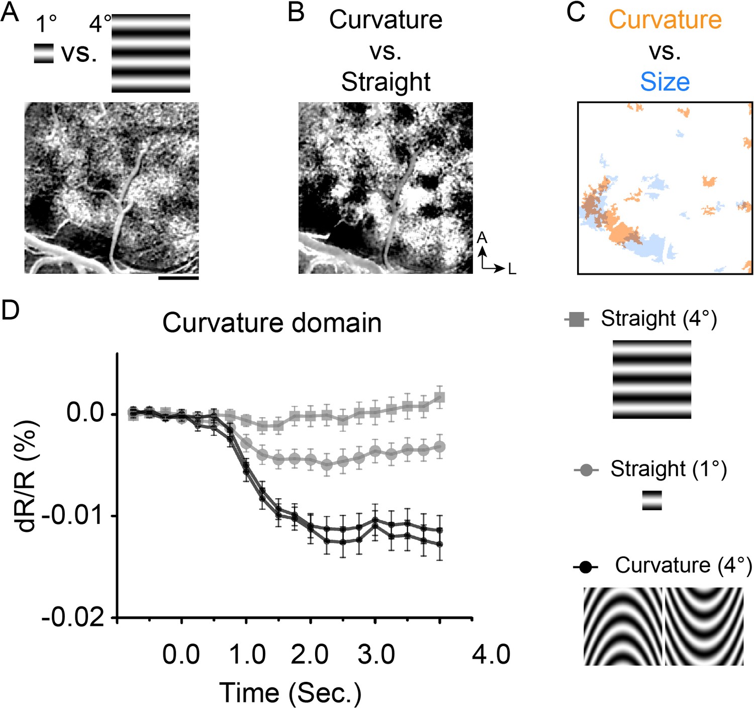
(A) Suppression domains: Subtraction image in response to small (1°, dark pixels) minus large (4°, light pixels) horizontal grating stimuli. (B) Curvature domains: Curvature map: all curved minus all straight. (C) Overlay: Locations of curvature domains (orange, from B, two tailed t test, p<0.01) and small size preferring domains (blue, from A, two tailed t test, p<0.01). There are overlapping and non-overlapping pixels between these two sets of pixels (overlapping: 33.3%, non-overlapping: 66.7%). (D) Response timecourses of curvature domains show poor response to small straight gratings (gray line square dot), slightly better response to large straight gratings (gray line round dot), and far better response to curvature gratings (black lines).
Figure 3 with 2 supplements
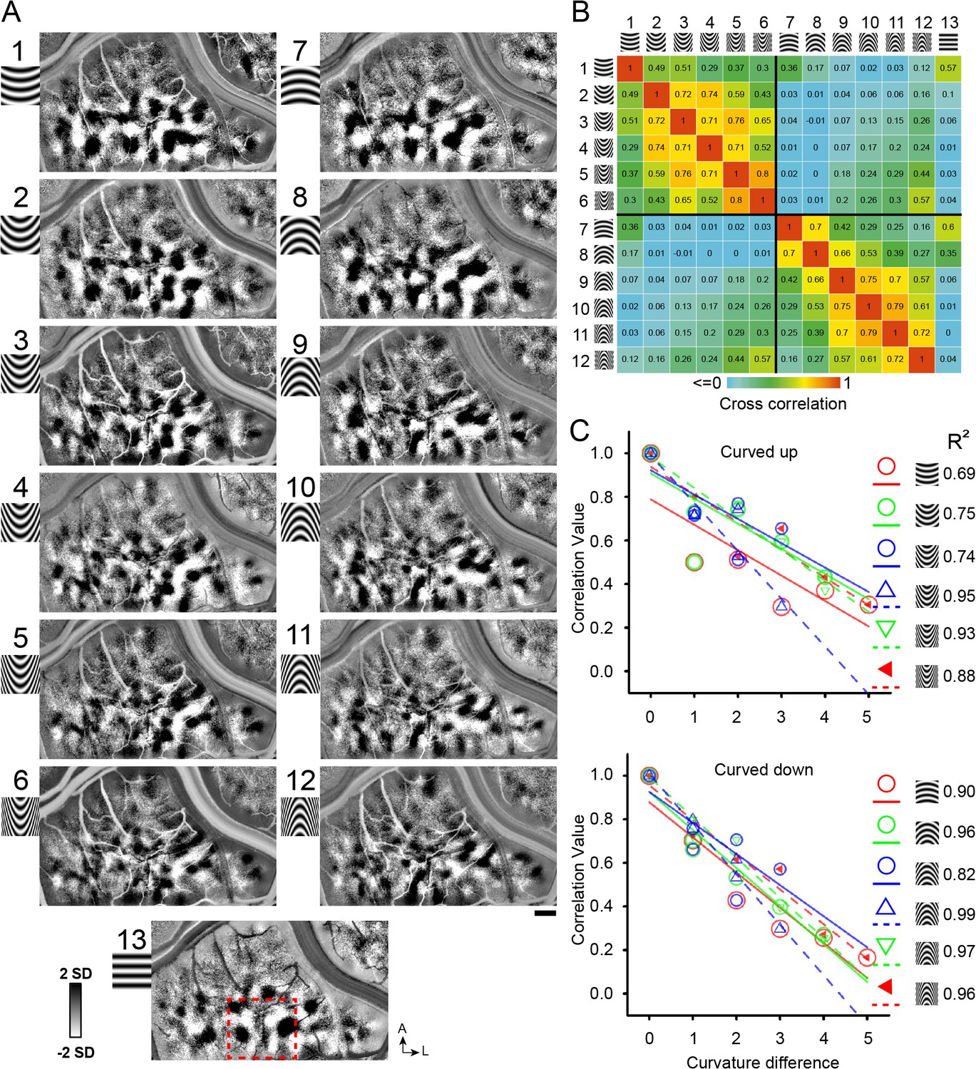
Systematic maps of curvature degree.
(A) Maps of different curvature degrees. Each map is one curvature minus average of all straight gratings (Case 1). 1–6 and 7–12: upwards and downwards curvatures, respectively, from low to high curvature preference, 13: straight grating. Red dotted square marks the region that is further analyzed in Figure 7A,B. Correlation values for pairs of curvature response maps (from A). Color bar: high (red) to low (blue) correlation values. (C) The more similar the curvature the greater the correlation value. X axis: curvature degree difference. Y axis: correlation value. Color symbols: correlation value for each curvature above with respect to its curvature degree distances (each fit with matching color line; regression values are shown on the right). The fitted lines are not meant to indicate linear fits; rather, they help to see the trends. Scale bar, 1 mm.
Figure 3—figure supplement 1
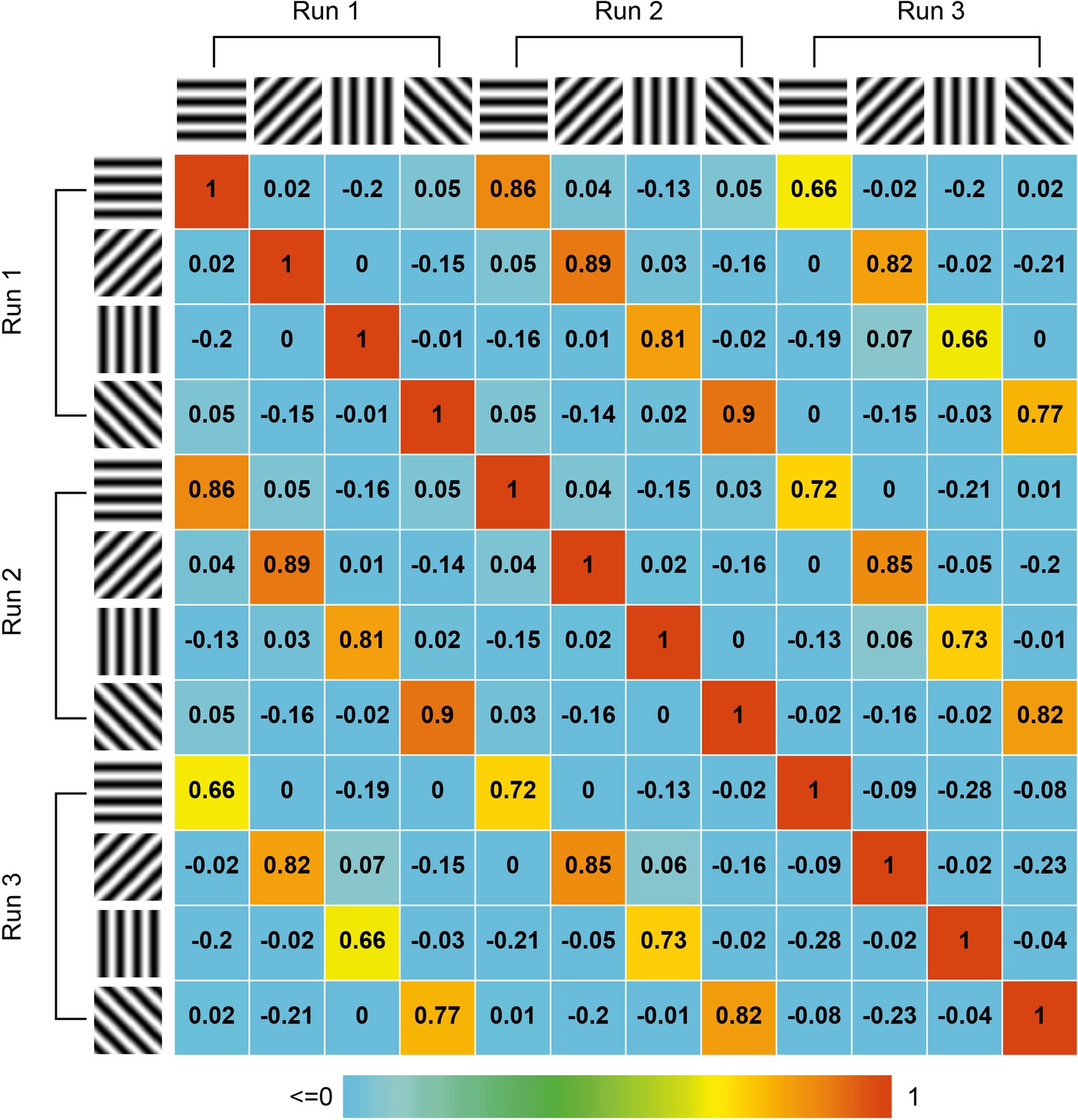
Correlation values between pairs of straight orientation maps obtained in three different runs (from Case 1).
These values are provided to give reader an idea of what high map correlations values are. When results from different runs are compared, only maps of similar orientation have high (orange, yellow) correlation values, while non-matching orientations produce low (blue) values. Color bar: correlation values (high, red, to low, blue) for pairs of maps. Note that negative values often occur for orthogonal orientations and are weaker in magnitude than positive values.
Figure 3—figure supplement 2

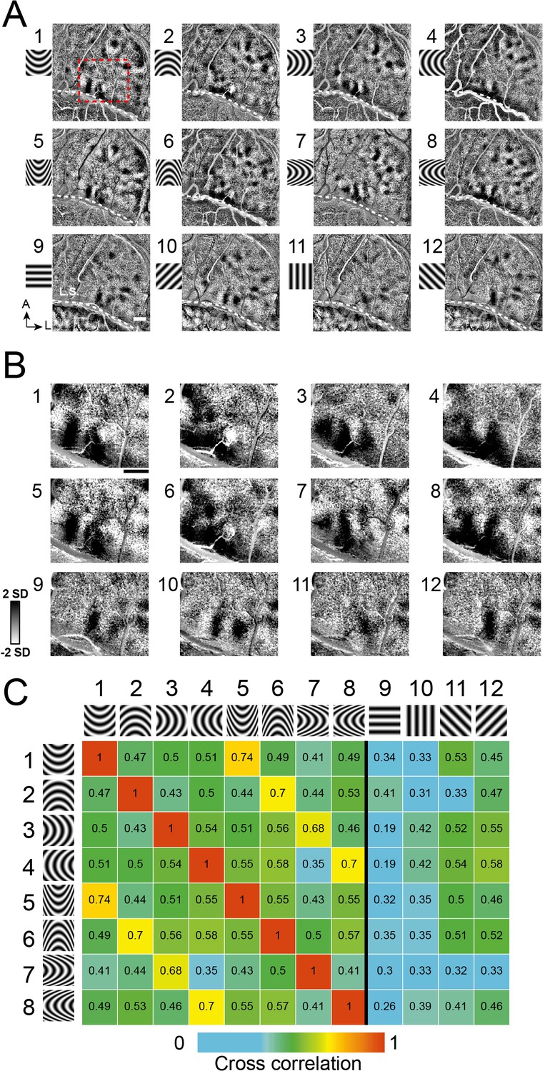
Systematic maps of curvature degree and curvature orientation in other cases.
(A) Case 2: Maps of different curvature degrees. (B) Correlation values for pairs of curvature response maps (from A). The more similar the curvature, the greater the correlation value (from B). (C) Case 1: Imaging maps of different curvature orientations. (D) Correlation values for pairs of curvature response maps (from C). Curvatures with the same orientation have greater correlation values (from D). Error bar: SEM. Scale bar: 1 mm. The correlation values are calculated based on the full data set (n=30 trials).
Figure 4
Systematic maps of curvature orientation.
(A) Imaging results of the responses to different curvature orientations. Maps of curvature minus average of straight gratings (Case 2). 1–4: low curvature degree, a/b ratio = 2, 5–8: high curvature degree, a/b ratio = 5. 1,5: upwards. 2,6: downwards. 3,7: leftwards. 4,8: rightwards. 9–12: straight. (B) Enlarged view of the cortical region outlined by red dotted box in A. (C) Correlation values for pairs of maps (from A). Maps of similar curvature orientation have high correlation values, while those with different curvature orientations have low correlation values. Colors code correlation values (high, red, to low, blue, see color bar).
Figure 5

Subregions of high curvature preference.
(A) Curvature preferring pixels. Red pixels: high curvature preferring pixels (high curvature vs. Low curvature, a/b ratio = 5 vs. 2, all four orientations, two-tailed t-test, p<0.01). White pixels: (curvature vs. straight). (Case 1: left, Case 2: right, two-tailed t-test, p<0.01). (B) High curvature subdomains (red pixels in A, Case 1) prefer high curvature (dark red lines, four orientations, a/b ratio = 5) over low curvature (light red lines, four orientations, a/b ratio = 2), and straight lines (Gray lines, four orientations). (C) Timecourses of response to 4 degrees of curvature (from high to low, darkest to lightest gray). Scale bar, 1 mm. Error bar: SEM.
Figure 6
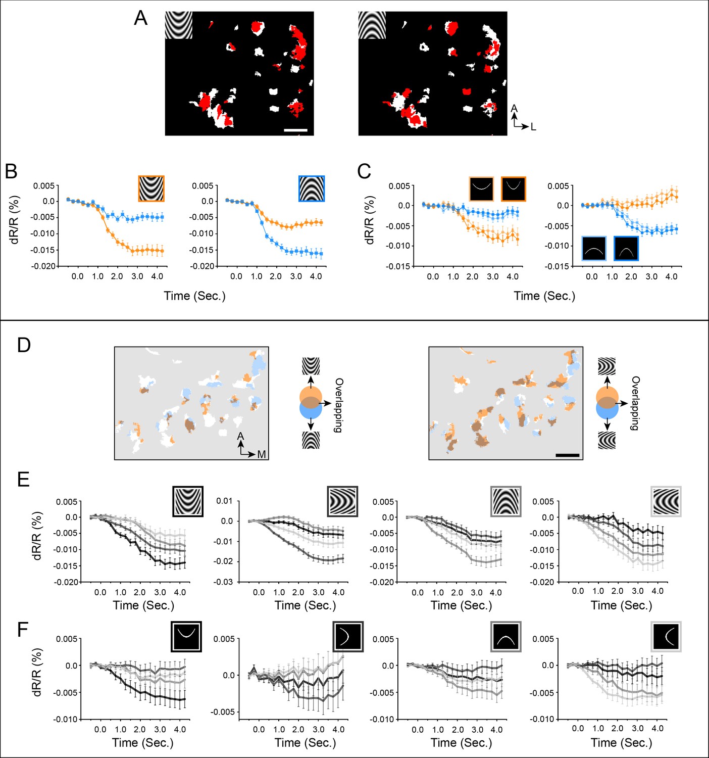
Organization of curvature orientation representation in V4 curvature domains (A-C: Case 2, D-F: Case 3).
(A) Curvature orientation maps (Case 2). White pixels: curvature vs. straight (two-tailed t test, p<0.01). Red pixels: significantly activated by different curvature orientations (compared to average of four straight orientations, two tailed t-test, p<0.01). There are overlapping as well as non-overlapping pixels between two opposite orientations. (B) Response timecourses of red pixels in A to curved gratings. (C) Response timecourses of the same red pixels in A to curved single lines. Orange lines: responses to up curvature, Blue lines: responses to down curvatures. For flashed curved lines, we used two different curvature degrees. (D) Curvature orientation maps (Case 3). White pixels: curvature vs. straight (two-tailed t test, p<0.01). Colored pixels: significantly activated by different curvature orientations. (E) Response timecourses of colored pixels in maps above to curved gratings. (F) Response timecourses of colored pixels in maps above to single flashed curved lines. Black lines: response timecourses to upwards curvature. Dark gray lines: response timecourses to leftwards curvature. Gray lines: response timecourses to downwards curvature. Light gray lines: response timecourses to rightwards curvature. Comparison of E and F graphs show that the orientation of the best curved grating response matches that of the best curved line response (gray timecourses). Scale bar: 1 mm. Error bar: SEM.
Figure 7 with 2 supplements
Functional organization of curvature in V4.
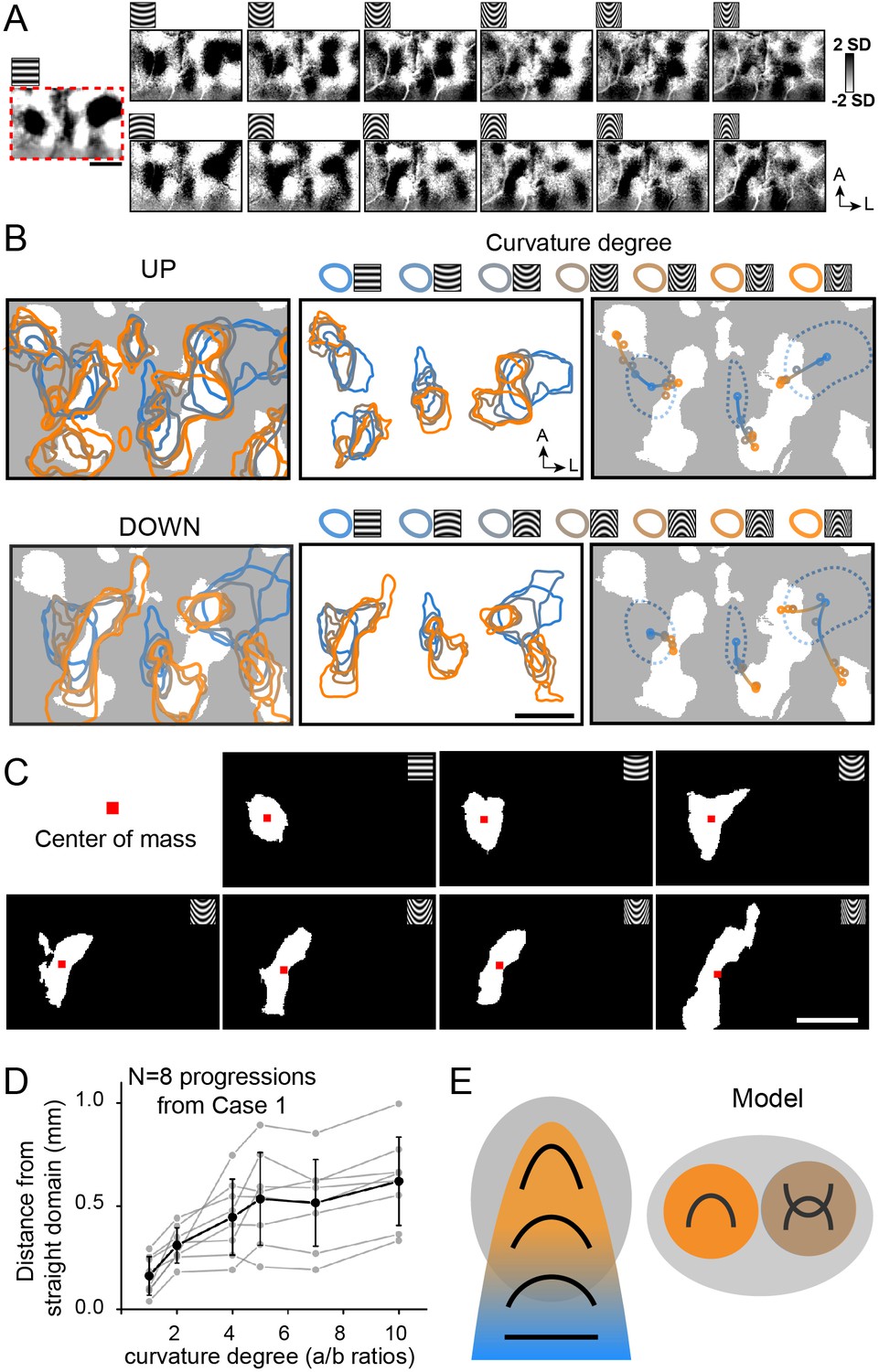
(A) Maps of different stimuli minus average of straight gratings (Case 1). Top row: upwards curvatures, bottom row: downwards curvatures. Leftmost: horizontal gratings. (B) Maps of progressions from straight to curved representation. Top row: responses to upwards curvatures (Up). Bottom row: responses to downwards curvatures (Down). Left panels: activated regions (two-tailed t-test, p<0.01) corresponding to different curvature stimuli. White regions: curvature domains. Color code: high (orange) to low (blue). Middle panels: activated regions corresponding (two-tailed t test, p<0.01, curved vs. average of straight) to respective curvature degrees are outlined by different colors (domain clusters are separated for clarity). Color code (at top): high (orange) to low (blue). [Note that the two leftmost domain progressions in Up panel are associated with the same orientation domain but are separated for clarity.] Right panels: Location of the activation center of each domain (indicated by colored dot). White regions: curvature domains. Blue dotted lines: horizontal orientation domains. Shifting progressions from straight orientation (blue dot) to low curvature (blue-orange dot) to high curvature (orange dot) are observed, as indicated by colored line (shaded from blue to orange). (C) Regions that were significantly activated (two-tailed t test, p<0.01) by corresponding stimuli (from Case 1). Red dots: centers of mass. (D) We measured the distance between each curvature domain activation center of mass and its corresponding straight orientation domain center of mass (a/b rations: 1, 2, 4, 5, 7, 10 in Case 1, eight progressions). Gray dots and lines: results from different progressions, black dots: averaged across all eight progressions. Error bar, SD. (E) Summary of curvature domain findings. Left: curvature degree progressions, Right: presence of curvature domains and complex curvature domains. Gray oval: curvature domains.
Figure 7—figure supplement 1
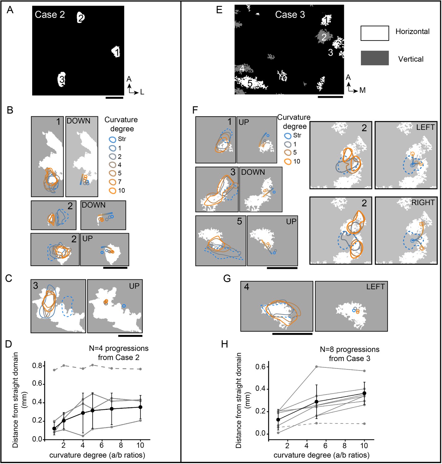
Diversity of curvature domain organization (A-D: Case 2, E-H: Case 3).
(A) In Case 2, we examined maps of horizontal straight to curved domains; the three straight domains are marked 1–3. (B) Curvature domains associated with Domain one and Domain two are outlined (Domain 2 associated with two progressions, one UP and one DOWN). The corresponding centers of mass are marked by colored circles (same as in Figure 7). White regions: curvature domains. (D) We measured the distance between each curvature domain activation center of mass and its straight orientation domain center of mass (a/b ratios: 1, 2, 4, 5, 7, 10; four progressions). Gray dots and lines: results from different progressions in B, black dots and lines: averaged across all three progressions in B. Error bar: SD. (E) In Case 3, we examined progressions of horizontal (1, 3, 5) and of vertical (2) straight to curved domains. (F, H) Same conventions as B, D. (F) Domains 1,3,5 are UP, DOWN, UP progressions, respectively. Domain 2 has two progressions for LEFT and two progressions for RIGHT; thus, it was associated with a total of four progressions. (H) a/b rations: 1, 5, 10; eight progressions. Gray dots and lines: results from different progressions in F, black dots and lines: averaged across all seven progressions in F. (C, G) Two examples of progressions that did not show domain shifts. C from Case 2: the curvature domains are highly overlapped and spatially separate from the straight orientation domain (dotted blue line) (dotted gray line in D); G from Case 3: the curvature domains and the straight orientation domain overlie the same position (dotted gray line in H).
Figure 7—figure supplement 2
Curvature domain response is not due to component orientation response.
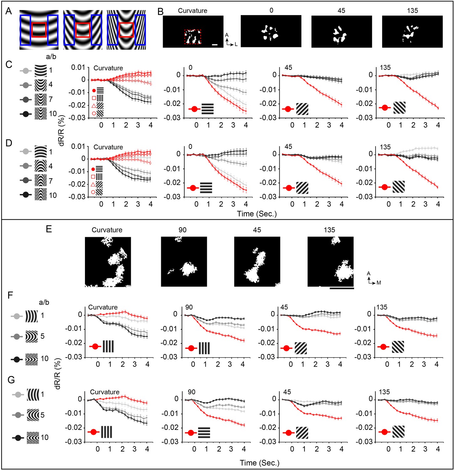
We compared the curvature response to three prominent component responses (0, 45, 135 deg as revealed by Fourier 2D transform). Three reasons why it is unlikely that curvature domain response is due to component response: (1) Curvature domains and orientation domains are spatially distinct (2) Curvature domains respond weakly to component orientations (by roughly an order of magnitude) and (3) orientation domains are weakly activated by curvature stimuli, only curvature domains show strong response (A-D: Case 1, E-G: Case 3). (A) Component orientations in the stimuli. Central (red) and flanking parts (blue) of the curvature stimuli. (B) Functional domains from the FOV in Figure 7E (red dotted rectangle). From left to right: curvature domains (all curved minus all straight), 0 deg, 45 deg, 135 deg orientation domains. (C, D) Response timecourses. In each of the curvature panels, these red lines correspond to the three orientations (horizontal, 45, 135). In each of the orientation panels, red lines correspond to the optimal orientations of the orientation domains (shown in the corner of each panel). The gray lines correspond to the identified curvature stimuli. (E) Functional domains. From left to right: curvature domains (all curved minus all straight), 90 deg, 45 deg domains, 135 deg orientation domains. (F, G) Response timecourses. Gray lines: see legend at left. Red lines: see legend within graph. Not due to a weighted sum. To do a quick calculation of a weighted sum of 0, 45, 135 orientation response. For upwards curvature (from C, a/b ratio = 7), Response0 = −0.0026%, Response45 = −0.0027%, Response135 = 0.0006%, Wi = 1/3, Response = −0.0016%, much weaker (by almost an order of magnitude) than the response in curvature domains −0.0115% (responses were calculated by average of the response amplitudes from the last 10 frames). While we are not able to test the weighted sum of all possible orientations, at least with this simple test, we do not see any indication of component summation.
Author response image 1
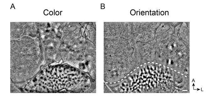
Clear functional maps of Case 2 from a different experiment session.
A. Color map. B. Orientation map.
Tables
Table 1
Case list.
| Case 1 | Case 2 | Case 3 | ||
|---|---|---|---|---|
| Curvature vs. straight map | Three cases (from three hemispheres of two animals) | Figure 2C and Figure 2—figure supplement 5B | Figure 2—figure supplement 4F,G and Figure 2—figure supplement 5C,D | Figure 2—figure supplement 6B |
| Curvature domain mask | Three cases | Figure 2G red pixels | Figure 5A right panel | Figure 6D |
| Curvature degree map | Three cases | Figure 3 | Figure 3—figure supplement 2A and B | Figure 7—figure supplement 1 |
| Curvature orientation map | Three cases | Figure 3—figure supplement 2C,D | Figure 4 and 6A | Figure 6D |
| Response consistency (curvature orientation) | Two cases (from two hemispheres of two animals) | NA | Figure 6A–C | Figure 6D–F |
| Scrambled response | One case | NA | NA | Figure 2—figure supplement 6 |
| Data used for response amplitude calculation | Cases 1 and 3 are from the same monkey. Response to color (Case 1: 50 trials; Case 2: 70 trials; Case 3: 50 trials with two different orientations) Response to high SF (Case 1: 80 trials; Case 2: 120 trials; Case 3: 100 trials with four different orientations) Response to 0, 45, 90, 135 (Case 1: 30 trials; Case 2: 30 trials; Case 3: 30 trials with the corresponding optimal orientations) Response to curvature grating (Case 1: 240 trials; Case 2: 240 trials; Case 3: 240 trials with four different curvature orientations and two different curvature degrees, a/b ratio 2 and 5) Response to flashed curvature (Case 2: 60 trials with two different curvature orientations; Case 3: 120 trials with four different curvature orientations) Number of pixels related to color domain (Case 1: 34986; Case 2: 10886; Case 3: 22560) Number of pixels related to high SF domain (Case 1: 31,480; Case 2: 10,687; Case 3: 29,757) Number of pixels related to 0, 45, 90, 135 orientation domain (Case 1: 33,676, 47,501, 51,798, 43,837; Case 2: 8225, 10,243, 4712, 8891; Case 3: 38,362, 31,651, 41,822, 41,466) Number of pixels related to curvature domain (Case 1: 30,215; Case 2: 18,209; Case 3: 24,351) | |||
Additional files
Download links
A two-part list of links to download the article, or parts of the article, in various formats.
Downloads (link to download the article as PDF)
Open citations (links to open the citations from this article in various online reference manager services)
Cite this article (links to download the citations from this article in formats compatible with various reference manager tools)
Curvature domains in V4 of macaque monkey
eLife 9:e57261.
https://doi.org/10.7554/eLife.57261


