Allosteric mechanism for KCNE1 modulation of KCNQ1 potassium channel activation
- Center for Structural Biology, Vanderbilt University, United States
- Department of Chemistry, Vanderbilt University, United States
- Institute for Drug Discovery, Leipzig University, Germany
- Department of Pharmacology, Northwestern University Feinberg School of Medicine, United States
- Department of Biochemistry, Vanderbilt University, United States
- Department of Pharmacology, Vanderbilt University, United States
Figures
Figure 1
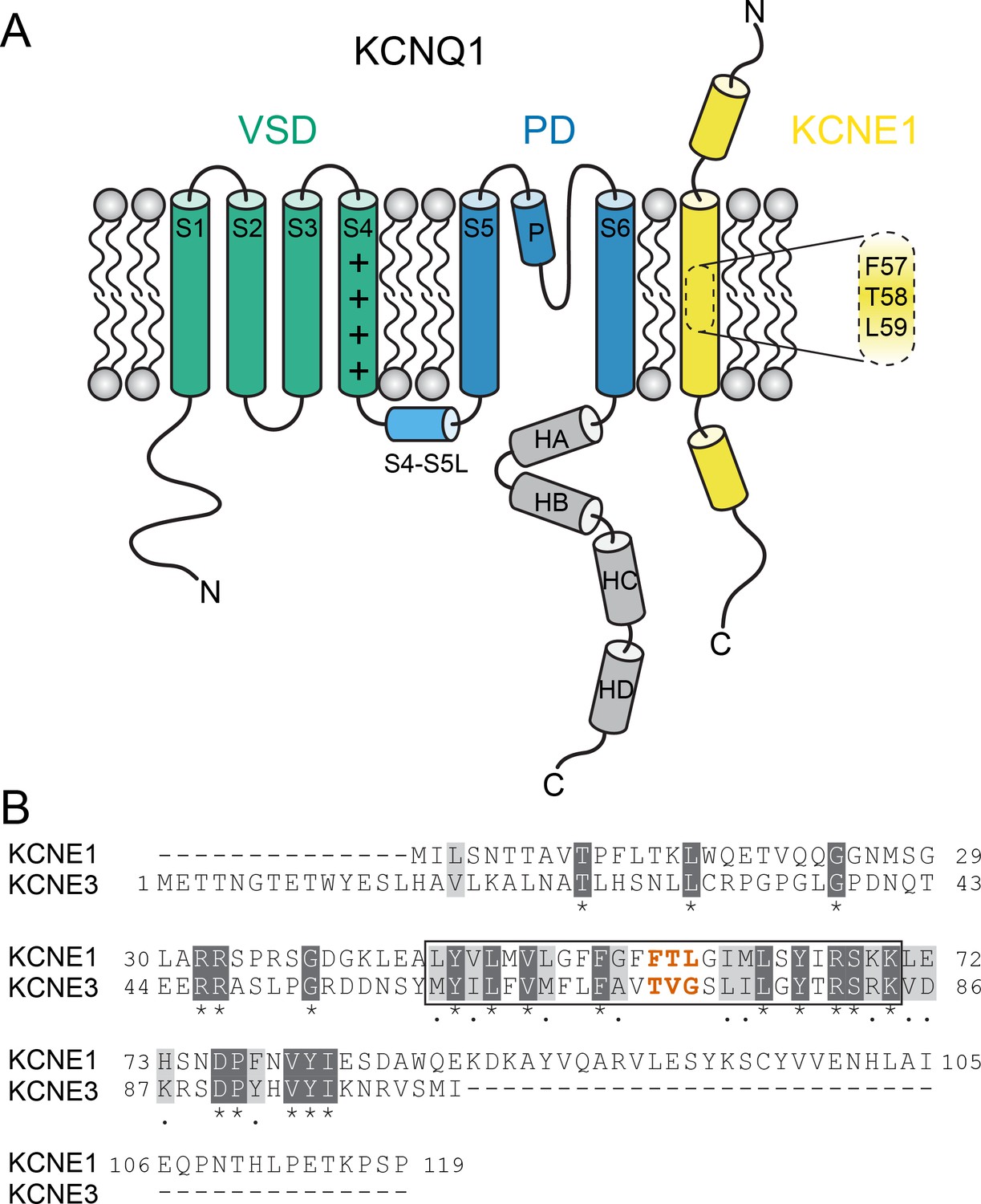
KCNQ1 channel architecture and sequence of KCNE proteins.
(A) Topology diagram of the KCNQ1-KCNE1 channel complex. The KCNQ1 voltage-sensing (VSD, helix S1-S4), pore-forming (PD, S5–P–S6), and cytosolic domains (helix HA-HD) are colored green, blue, and gray, respectively. KCNE1 exhibits a single-span transmembrane domain (TMD) that is flanked by intra- and extracellular domains containing helical segments. (B) Amino acid sequence alignment of KCNE1 and KCNE3. Similar and identical amino acid residues are colored light and dark gray, respectively. The TMD region is indicated by a black box. The activation motif regions in KCNE1 and KCNE3 are highlighted in red.
Figure 2 with 3 supplements
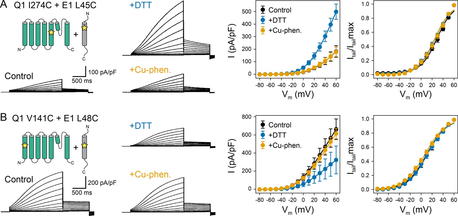
Oxidation state-dependent electrophysiology measurements indicate that KCNQ1 V141 and I274 are close to L48 and L45 in KCNE1, respectively.
(A) Whole-cell currents (left) and average current-voltage (I–V) relationships (right) of CHO-K1 cells transiently expressing KCNQ1 I274C and KCNE1 L45C. Cells were exposed to control bath solution containing DTT or Cu-phenanthroline (Cu-phen.). (mean ± SEM, Control n = 6, DTT n = 6, Cu-phen n = 5). (B) Whole-cell currents (left) and average I-V relationships (right) of CHO-K1 cells expressing KCNQ1 V141C and KCNE1 L48C, which were exposed to control bath solution, DTT, or Cu-phenanthroline, respectively. (Control n = 7, DTT n = 5, Cu-phen n = 5). Solid lines represent fits with a Boltzmann function (Itail/Itailmax = (1-IBottom) / (1+exp[(V1/2app-V)/k]) + IBottom) and the parameters of the fit are summarized in Supplementary file 1 – Table 1. Control measurements of KCNQ1 WT, V141C, and I274C with and without KCNE1 under reducing (+DTT) and oxidizing (+Cu-phen.) conditions are displayed in Figure 2—figure supplement 1 and Figure 2—figure supplement 2.
-
Figure 2—source data 1
Excel file with numerical electrophysiology data used for Figure 2.
- https://cdn.elifesciences.org/articles/57680/elife-57680-fig2-data1-v1.xlsx
Figure 2—figure supplement 1
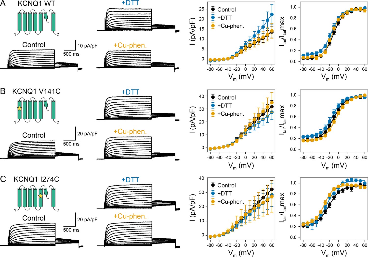
Electrophysiology measurements of KCNQ1 WT, V141C, and I274C under reducing and oxidizing conditions.
(A) Whole-cell currents (left) and average I-V relationships (right) of CHO-K1 cells expressing KCNQ1 WT, which were exposed to control bath solution, DTT, or Cu-phenanthroline (Cu-phen.), respectively. (mean ± SEM, Control n = 9, DTT n = 5, Cu-phen. n = 5) (B) Whole-cell currents and average I-V relationships of CHO-K1 cells expressing KCNQ1 V141C, which were exposed to control bath solution containing DTT or Cu-phenanthroline. (Control n = 13, DTT n = 7, Cu-phen. n = 5) (C) Whole-cell currents and average I-V relationships of CHO-K1 cells expressing KCNQ1 I274C measured with or without DTT or Cu-phenanthroline in the bath solution. (Control n = 12, DTT n = 7, Cu-phen. n = 7) Solid lines represent fits with a Boltzmann function (Itail/Itailmax = (1 - IBottom) / (1+exp[(V1/2app - V)/k]) + IBottom) and the parameters of the fit are summarized in Supplementary file 1 – Table 1.
-
Figure 2—figure supplement 1—source data 1
Excel file with numerical electrophysiology data used for Figure 2—figure supplement 1.
- https://cdn.elifesciences.org/articles/57680/elife-57680-fig2-figsupp1-data1-v1.xlsx
-
Figure 2—figure supplement 1—source data 2
Excel file with numerical electrophysiology data used for Figure 2—figure supplement 2.
- https://cdn.elifesciences.org/articles/57680/elife-57680-fig2-figsupp1-data2-v1.xlsx
-
Figure 2—figure supplement 1—source data 3
Excel file with numerical electrophysiology data used for Figure 2—figure supplement 3.
- https://cdn.elifesciences.org/articles/57680/elife-57680-fig2-figsupp1-data3-v1.xlsx
Figure 2—figure supplement 2
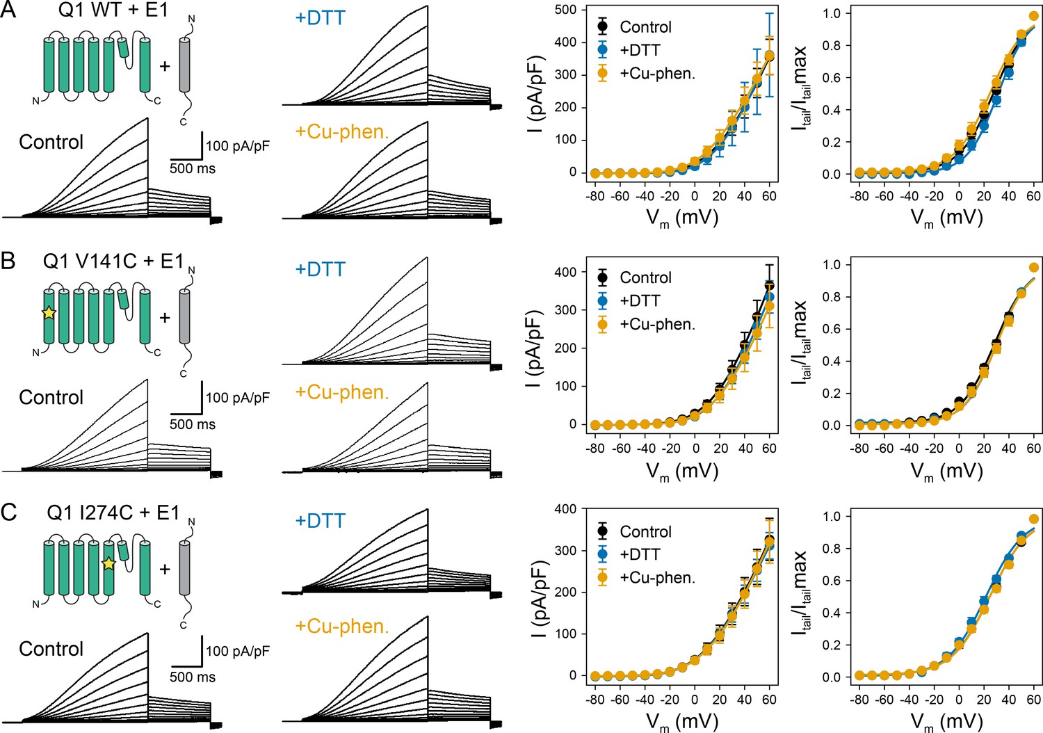
Electrophysiology measurements of KCNQ1 WT, V141C, and I274C with KCNE1 WT under reducing and oxidizing conditions.
(A) Whole-cell currents (left) and average I-V relationships (right) of CHO-K1 cells expressing KCNQ1 and KCNE1 WT, which were exposed to control bath solution, DTT, or Cu-phenanthroline (Cu-phen.), respectively. (mean ± SEM, Control n = 10, DTT n = 4, Cu-phen. n = 6) (B) Whole-cell currents and average I-V relationships of CHO-K1 cells expressing KCNQ1 V141C and KCNE1 WT, which were exposed to control bath solution containing DTT or Cu-phenanthroline. (Control n = 18, DTT n = 12, Cu-phen. n = 9) (C) Whole-cell currents and average I-V relationships of CHO-K1 cells expressing KCNQ1 I274C and KCNE1 WT measured with or without DTT or Cu-phenanthroline in the bath solution. (Control n = 20, DTT n = 9, Cu-phen. n = 11) Solid lines represent fits with a Boltzmann function (Itail/Itailmax = (1 - IBottom) / (1+exp[(V1/2app - V)/k]) + IBottom) and the parameters of the fit are summarized in Supplementary file 1 – Table 1.
Figure 2—figure supplement 3
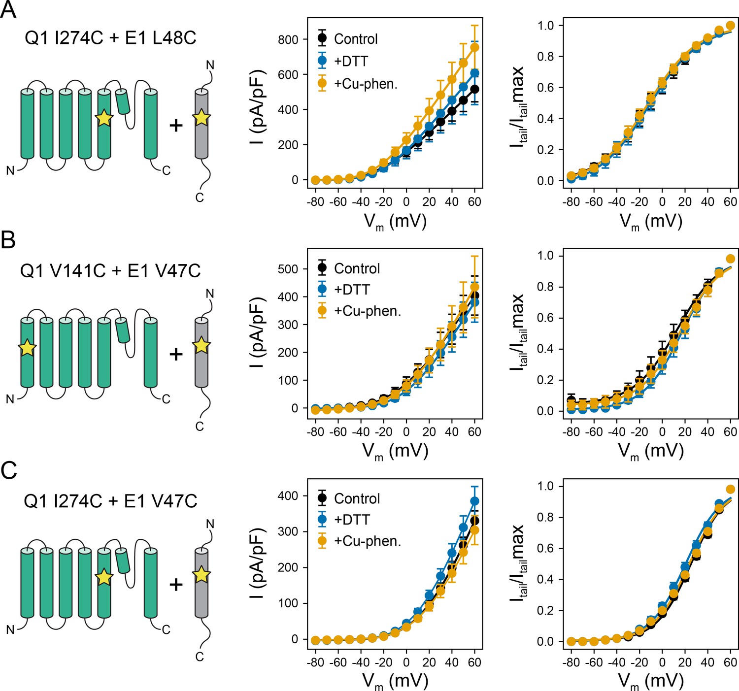
Electrophysiology measurements of KCNQ1 V141C or I274C with KCNE1 V47C or L48C under reducing and oxidizing conditions.
(A) Average I-V relationships and activation curves of currents recorded from CHO-K1 cells transiently expressing KCNQ1 I274C and KCNE1 L48C. Cells were exposed to control bath solution, DTT, or Cu-phenanthroline (Cu-phen.), respectively. (mean ± SEM, Control n = 12, DTT n = 7, Cu-phen. n = 7) (B) Average I-V relationships and activation curves of currents measured from CHO-K1 cells transiently expressing KCNQ1 V141C and KCNE1 V47C, which were exposed to control bath solution, DTT, or Cu-phenanthroline (Cu-phen.), respectively. (mean ± SEM, Control n = 13, DTT n = 10, Cu-phen. n = 7) (C) Average I-V relationships and activation curves of CHO-K1 cells expressing KCNQ1 I274C and KCNE1 V47C with and without DTT or Cu-phenanthroline in the bath solution. (Control n = 8, DTT n = 6, Cu-phen n = 6) Solid lines represent fits with a Boltzmann function (Itail/Itailmax = (1 - IBottom) / (1+exp[(V1/2app - V)/k]) + IBottom) and the parameters of the fit are summarized in Supplementary file 1 – Table 1.
Figure 3 with 4 supplements
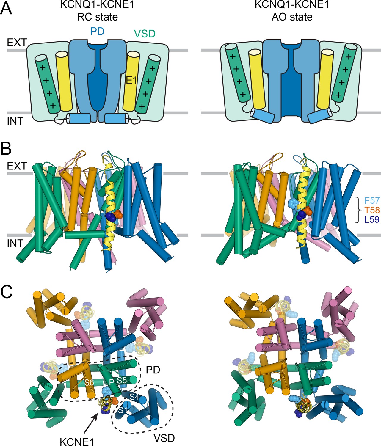
Molecular models of the KCNQ1-KCNE1 channel in RC and AO conformations.
(A) Schematic cartoon depicting the functional states of the VSD (green box) and PD (blue box) in the KCNQ1-KCNE1 models. The S4 helix (with positive gating charges “+”) and S4-S5L, which connects S4 to the PD, are shown as green and blue cylinders, respectively. KCNE1 was docked to KCNQ1 with the VSD/PD in the resting/closed (RC) or activated/open (AO) conformation. (B) Side view of the KCNQ1-KCNE1 docking models. KCNQ1 is represented with cylindrical helices and KCNE1 is depicted as yellow ribbon. Residues F57, T58, and L59 are drawn as spheres and colored light blue, red, and dark blue, respectively. The approximate position of the membrane bilayer is indicated by horizontal lines and the extracellular and intracellular side are labeled EXT and INT, respectively. (C) View of the KCNQ1-KCNE1 models from the extracellular side. KCNE1 is bound in a cleft between the VSD and PD and makes contacts to three KCNQ1 subunits. The position of the other three equivalent KCNE1-binding sites in the tetrameric KCNQ1 channel is indicated.
Figure 3—figure supplement 1
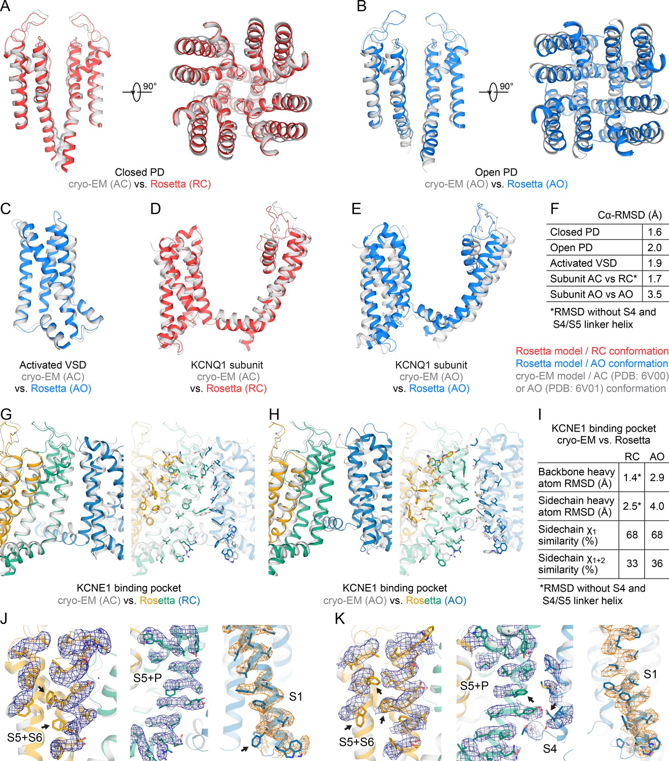
Structural comparison of Rosetta-generated computational models of human KCNQ1, which were used for docking, with cryo-EM-determined models of human KCNQ1 (Sun and MacKinnon, 2020).
(A) Comparison of the PD from the Rosetta model of the resting/closed (RC) state with the PD from the cryo-EM model of the activated/closed (AC) conformation (PDB: 6V00). (B) Comparison of the PD from the Rosetta model of the activated/open (AO) state with the PD from the cryo-EM model of the AO conformation (PDB: 6V01). (C) Comparison of the VSD in an activated conformation from the Rosetta AO model with the VSD from the cryo-EM AC model (PDB: 6V00). (D) Comparison of one KCNQ1 subunit from the Rosetta RC model with the corresponding subunit from the cryo-EM AC model (PDB: 6V00). The RMSD was calculated excluding the S4 and S4-S5L helix because those two helices undergo conformational changes during transition from the resting (RC) to the activated (AC) state. (E) Comparison of one KCNQ1 subunit from the Rosetta AO model with the corresponding subunit from the cryo-EM AO model (PDB: 6V01). (F) Summary of the Cα-RMSD values (in Å) calculated for the structural comparisons in (A) to (E). (G) Comparison of the KCNE1-binding pocket from the Rosetta RC model with that from the cryo-EM AC model (PDB: 6V00). Surface-exposed sidechains are represented as sticks in the right panel. (H) Comparison of the KCNE1 binding pocket from the Rosetta AO model with that from the cryo-EM AO model (PDB: 6V01). (I) Summary of the backbone and sidechain RMSD values and rotamer similarity for surface-exposed residues depicted in the structural comparisons in (G) and (H). (J) Close-up views of surface-exposed residues in the KCNE1-binding region depicted in (G). Sidechain conformations in the Rosetta RC model are compared with those in the cryo-EM AC model and with the cryo-EM density map (EMD: 20966). Sidechains with a rotamer state that does not fit into the density are indicated with an arrow. (K) Close-up views of surface-exposed residues in the KCNE1-binding region depicted in (G). Sidechain conformations in the Rosetta AO model are compared with those in the cryo-EM AO model and with the cryo-EM density map (EMD: 20967).
Figure 3—figure supplement 2
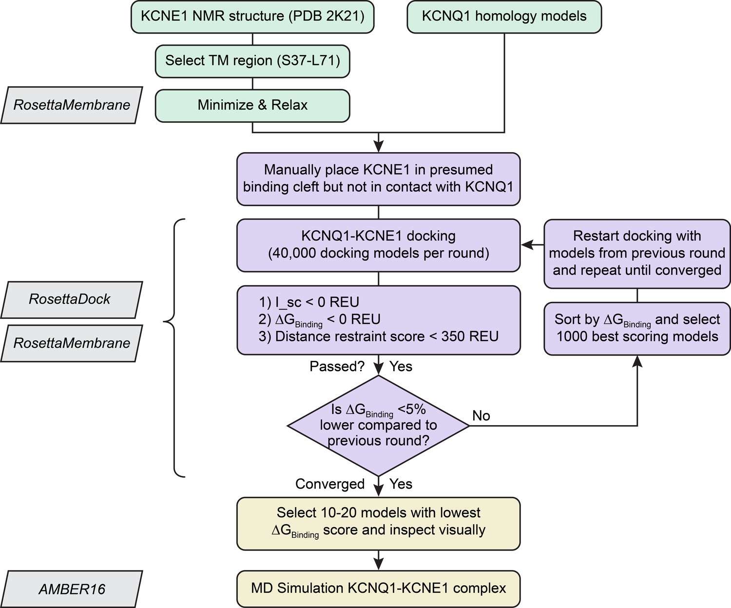
Flowchart of the Rosetta protein-protein docking protocol for building KCNQ1-KCNE1 models.
Modeling was conducted in three stages: preparation of KCNE1 input structures and KCNQ1 homology models, iterative protein-protein docking and distance restraint score-based filtering for model generation, and visual model inspection and MD simulation for model analysis. Individual modeling steps are written within rounded rectangular boxes whereas the names of used algorithms and programs are within skewed rectangular boxes. Compare also with Materials and method details.
Figure 3—figure supplement 3
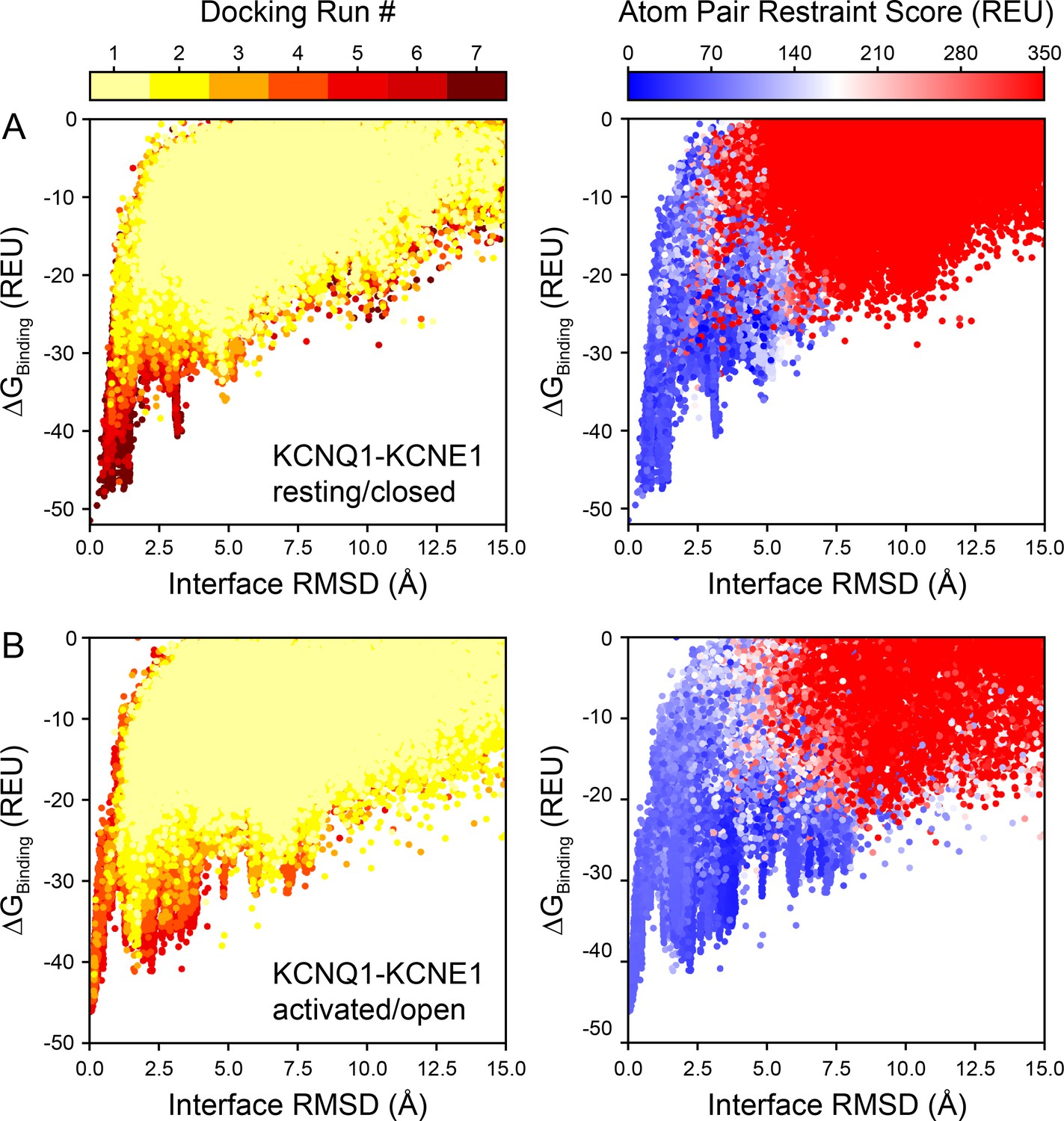
Rosetta binding energy (ΔGBinding) versus interface root-mean-square deviation (RMSD) plots of KCNQ1-KCNE1 docking models.
For every model of KCNE1 docked to KCNQ1 in (A) the resting/closed or (B) activated/open conformation, the Rosetta binding energy (ΔGBinding) and protein-protein interface RMSD relative to the best scoring model is plotted. Colors represent the docking round (left) or a model’s atom pair restraint score (right), respectively.
-
Figure 3—figure supplement 3—source data 1
Excel file with numerical data used for the energy-vs-RMSD plots in panel A of Figure 3—figure supplement 3.
- https://cdn.elifesciences.org/articles/57680/elife-57680-fig3-figsupp3-data1-v1.xlsx
-
Figure 3—figure supplement 3—source data 2
Excel file with numerical data used for the energy-vs-RMSD plots in panel B of Figure 3—figure supplement 3.
- https://cdn.elifesciences.org/articles/57680/elife-57680-fig3-figsupp3-data2-v1.xlsx
Figure 3—figure supplement 4
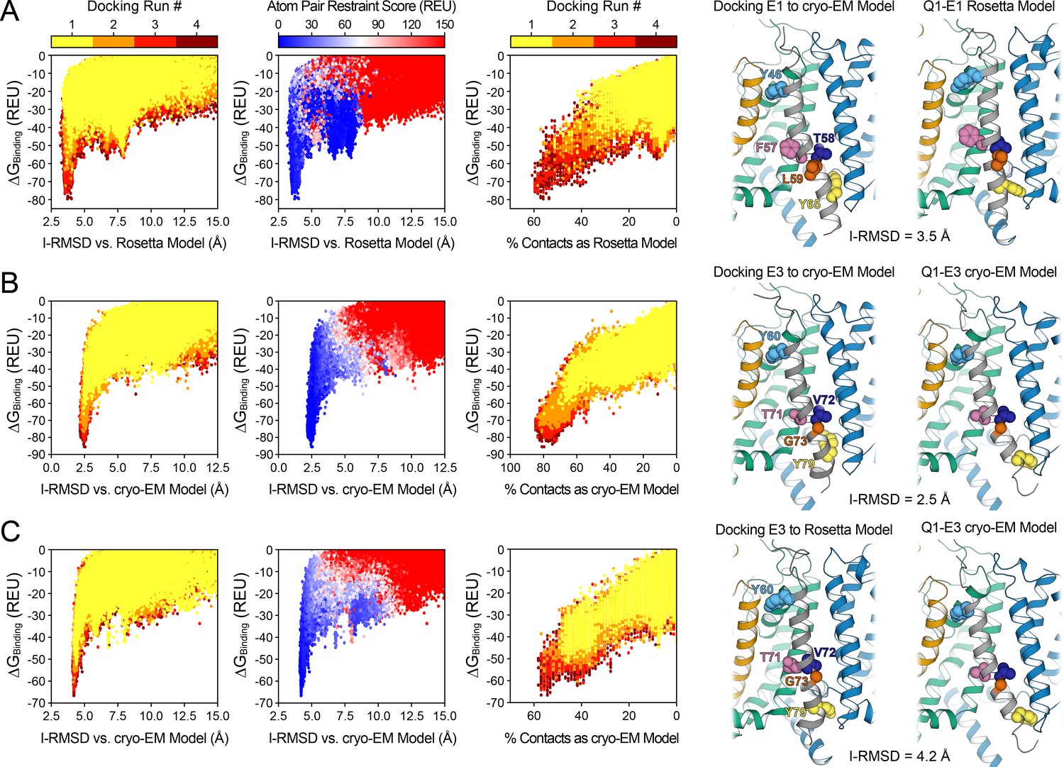
Control docking calculations for KCNQ1-KCNE1 and KCNQ1-KCNE3 complexes using the Rosetta and cryo-EM models of the activated/open state structure.
(A) Docking of the NMR-determined model of KCNE1 (S37–L71) (PDB: 2K21) (Kang et al., 2008) to the cryo-EM-determined open state model of KCNQ1 (PDB: 6V01) (Sun and MacKinnon, 2020). Left: Rosetta-binding energy (ΔGBinding) for KCNE1 versus the docking models’ interface RMSD (I-RMSD) and fraction of recovered contacts compared to the model developed by docking KCNE1 to the Rosetta homology model of the KCNQ1 open state structure. Right: Comparison of the best-scoring model obtained by docking KCNE1 to the cryo-EM model of KCNQ1 versus the Rosetta KCNQ1-KCNE1 model developed in this work. The I-RMSD between the two models is indicated. (B) Docking of the NMR-determined model of KCNE3 (P51–V85) (PDB: 2NDJ) (Kroncke et al., 2016) to the cryo-EM-determined open state model of human KCNQ1 (PDB: 6V01) (Sun and MacKinnon, 2020). Left: Rosetta binding energy for KCNE3 versus the docking models’ I-RMSD and fraction of recovered contacts compared to the cryo-EM model of the KCNQ1-KCNE3 complex. Right: Comparison of the best-scoring KCNQ1-KCNE3 docking model with the cryo-EM model of the KCNQ1-KCNE3 complex. (C) Docking of the NMR-determined model of KCNE3 (PDB: 2NDJ) (Kroncke et al., 2016) to the Rosetta homology model of the KCNQ1 open state structure. Left: Rosetta binding energy for KCNE3 versus the docking models’ I-RMSD and fraction of recovered contacts relative to the cryo-EM model of the KCNQ1-KCNE3 complex. Right: Structural model developed by docking KCNE3 to the Rosetta homology model compared to the cryo-EM-determined model for the KCNQ1-KCNE3 complex (PDB: 6V01) (Sun and MacKinnon, 2020).
-
Figure 3—figure supplement 4—source data 1
Excel file with numerical data used to make the energy-vs-I-RMSD plots in panel A of Figure 3—figure supplement 4.
- https://cdn.elifesciences.org/articles/57680/elife-57680-fig3-figsupp4-data1-v1.xlsx
-
Figure 3—figure supplement 4—source data 2
Excel file with numerical data used to make the energy-vs-I-RMSD plots in panel B of Figure 3—figure supplement 4.
- https://cdn.elifesciences.org/articles/57680/elife-57680-fig3-figsupp4-data2-v1.xlsx
-
Figure 3—figure supplement 4—source data 3
Excel file with numerical data used to make the energy-vs-I-RMSD plots in panel C of Figure 3—figure supplement 4.
- https://cdn.elifesciences.org/articles/57680/elife-57680-fig3-figsupp4-data3-v1.xlsx
Figure 4
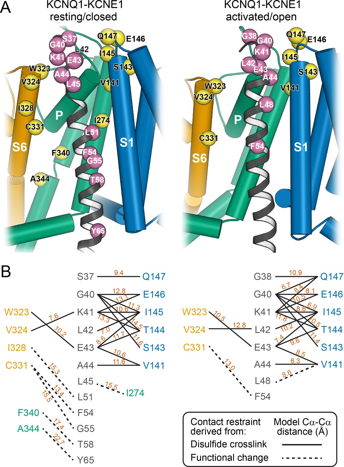
Mapping of experimental distance restraint sites onto the KCNQ1-KCNE1 models.
(A) Interaction of KCNE1 with the KCNQ1 RC and AO model in the transmembrane region. Residues whose distance was restrained in docking are indicated as spheres. (B) Restrained residue pairs and their Cα-Cα distances (in Å) in the KCNQ1-KCNE1 RC and AO models.
Figure 5 with 3 supplements
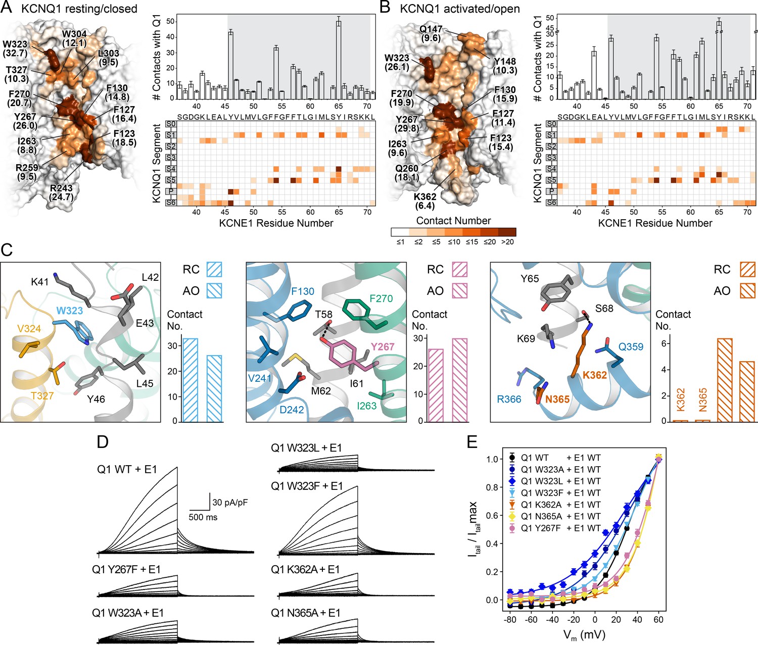
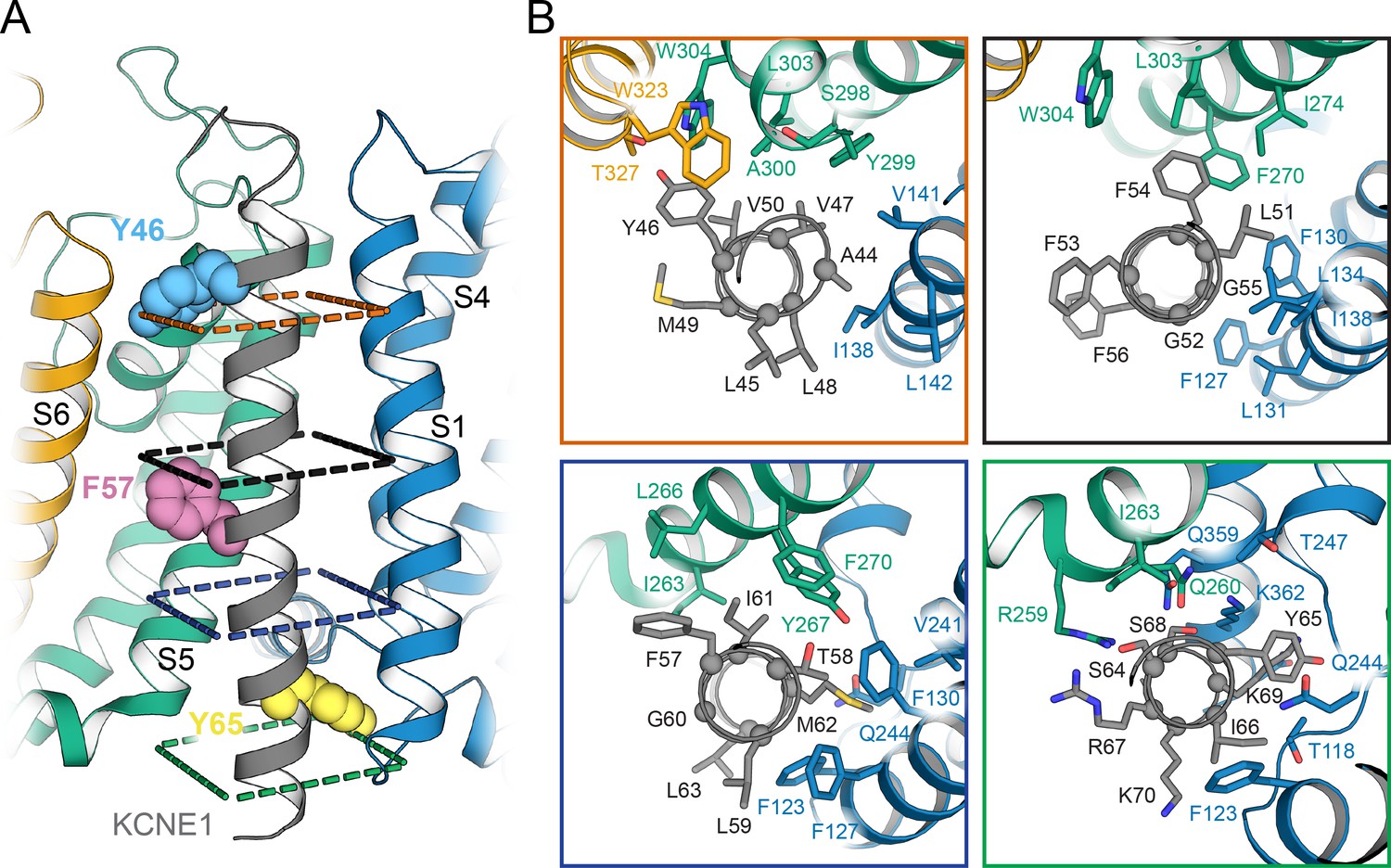
Computational detection and experimental validation of the KCNE1-binding site of KCNQ1.
(A) Left: Surface representation of the KCNE1 binding cleft in the KCNQ1 RC model. Residues are colored by their average MD contact number with KCNE1 (indicated in parentheses). Right: Matrix of KCNQ1-KCNE1 contacts (bottom) and histogram of the number of intermolecular contacts for KCNE1 (top) (mean ± SD). (B) Left: Surface representation of the KCNE1 binding site in the KCNQ1 AO model with residues colored by their average MD contact number. Right: Matrix and histogram of the number of intermolecular contacts for KCNE1 (mean ± SD). (C) Interaction of KCNQ1 with the upper, middle, and lower part of the KCNE1 TMD. Three selected sites in KCNQ1 and their neighboring residues in KCNQ1 and KCNE1 are displayed: left – W323, middle – Y267, right – K362+N365. Residue sidechains are drawn as sticks and potential H-bond contacts are indicated by dashed lines. Histograms of the average MD contact number with KCNE1 for the selected residues in the KCNQ1 RC and AO model are shown next to the structural models. (D) Whole-cell currents of CHO-K1 cells stably expressing KCNE1 and transfected with KCNQ1 WT or mutant cDNA. (E) Normalized activation curves for currents recorded from cells expressing KCNQ1 WT or mutants. (mean ± SEM, WT n = 45, W323A n = 22, W323L n = 25, W323F n = 58, Y267F n = 22, K362A n = 31, N365A n = 24).
-
Figure 5—source data 1
Excel file with numerical data used for panels A, B, and E of Figure 5.
- https://cdn.elifesciences.org/articles/57680/elife-57680-fig5-data1-v1.xlsx
Figure 5—figure supplement 1

MD simulations for the KCNQ1-KCNE1 RC and AO channel models.
(A) Side and extracellular views of the MD simulation box containing the KCNQ1-KCNE1 RC model. The KCNQ1-KCNE1 complex was embedded in a membrane bilayer containing 287 POPC molecules in the outer leaflet and 245 POPC and 28 PIP2 molecules in the inner leaflet. The system was hydrated with 53,265 water molecules and the charge was neutralized by adding 192 K+ and 146 Cl- ions (corresponds to 150 mM KCl). The KCNQ1-KCNE1 complex is shown in ribbon and surface representation. The lipid fatty acid chains are depicted by yellow sticks and the head group phosphates are represented as orange spheres. K+ and Cl- ions are displayed as gray and magenta spheres, respectively. (B) Side and extracellular views of the MD simulation box containing the KCNQ1-KCNE1 AO model. The KCNQ1-KCNE1 complex was embedded in a membrane bilayer containing 286 POPC molecules in the outer leaflet and 246 POPC and 28 PIP2 molecules in the inner leaflet. The system was hydrated with 47,051 water molecules and the charge was neutralized by adding 174 K+ and 128 Cl- ions (corresponds to 150 mM KCl). The same representation styles and colors for protein, lipids, and ions as in (A) are used. (C) Average Cα-atom RMSD for KCNQ1 and KCNE1 relative to the starting structure over the course of the MD trajectory. (D) Sidechain-sidechain distances between gating charge residues in S4 (R1–R6) and negatively charged residues in S2 (E160, E170) and S3 (D202) confirm the resting and activated VSD conformations in the KCNQ1 RC and AO model, respectively. Distances were measured between the geometric centers of the sidechain atoms: H2N = Cζ(NH2)-NεH-CδH2 (Arg), H3Nζ-CεH2 (Lys), Cγ-Nδ1-Cε1H-Nε2H-Cδ2H (His), HOOCγ-CβH2 (Asp), HOOCε-CγH2 (Glu). (E) Average pore radius of KCNQ1 calculated with the program HOLE (Smart et al., 1996). The shaded area corresponds to one standard deviation. The approximate radius of a K+ ion is indicated by a dashed line. Amino acid residues forming constriction sites along the channel pore are labeled. The region between 3 Å and 14 Å corresponds to the selectivity filter region.
-
Figure 5—figure supplement 1—source data 1
Excel file with numerical MD simulation data used for panels C, D, and E of Figure 5—figure supplement 1.
- https://cdn.elifesciences.org/articles/57680/elife-57680-fig5-figsupp1-data1-v1.xlsx
Figure 5—figure supplement 2
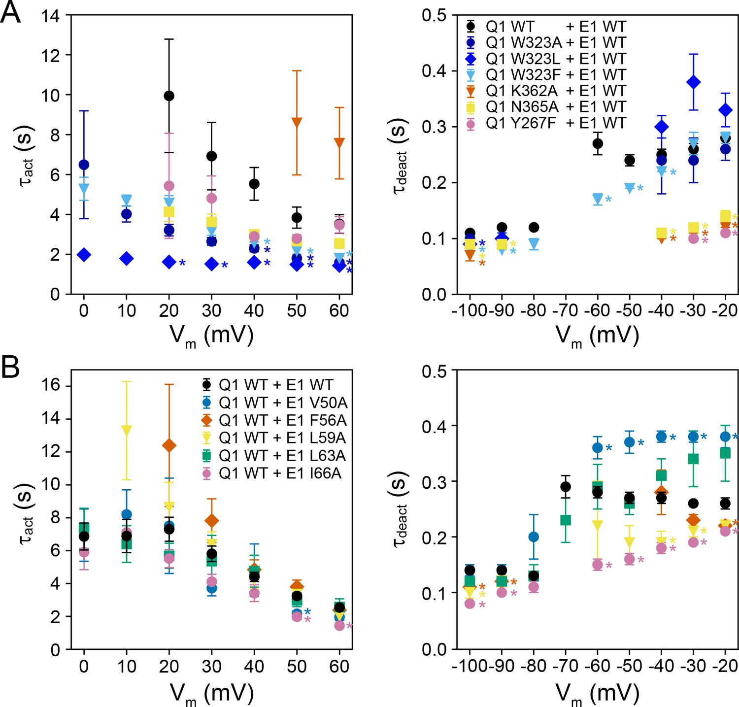
Activation (τact) and deactivation times (τdeact) of WT and mutant KCNQ1-KCNE1 channels.
(A) Activation and deactivation times from fits to currents recorded from channels formed by KCNQ1 mutants + KCNE1 WT. (mean ± SEM, WT n = 9–58 (τact)/17–63 (τdeact), W323A n = 6–48/5–12, W323L n = 5–50/6–19, W323F n = 27–70/9–56, K362A n = 9–17/6–17, N365A n = 13–55/8–17, Y267F n = 8–46/7–10) (B) Activation and deactivation times from fits to currents recorded from channels formed by KCNQ1 WT + KCNE1 mutants. (mean ± SEM, WT n = 56–293 (τact)/42–261 (τdeact), V50A n = 21–48/4–42, F56A n = 7–35/4–24, L59A n = 7–44/4–24, L63A n = 4–27/4–29, I66A n = 15–41/11–35). Activation and deactivation times for KCNQ1-KCNE1 channels with KCNE1 mutations at Y46, F57, and Y65, respectively, are shown in Figure 7A. Time constants significantly different from those of KCNQ1 WT + KCNE1 WT are indicated (*p<0.001, Student’s t-test).
Figure 5—figure supplement 3

Cartoon model for the interaction of KCNQ1 residues H363 and I368 with KCNE1 residues H73, S74, and D76.
Rosetta KCNQ1-KCNE1 RC model (A) and AO model (B) with extended C-terminal ends for KCNQ1 S6 and KCNE1. Residues that were identified in cysteine-crosslinking (Lvov et al., 2010) and double mutant cycle experiments (Chen et al., 2020) to be in proximity are depicted as spheres.
Figure 6 with 1 supplement
Orientation of the KCNE1 TMD in KCNQ1.
(A) Cartoon representation of the KCNE1 TMD and its surrounding helical segments in the KCNQ1 AO model. The KCNQ1-KCNE1 RC model is shown in Figure 6—figure supplement 1. Residues Y46, F57, and Y65, at which mutation to Ala or Leu led to a significant change in V1/2app of KCNQ1 activation (Figure 7), are drawn as spheres. (B) View of the KCNE1-KCNQ1 interface from the extracellular side at planes indicated in (A). KCNQ1-KCNE1 residue interactions in the RC and AO model are also shown in Videos 1 and 2, respectively.
Figure 6—figure supplement 1

Orientation of the KCNE1 TMD in the KCNQ1 RC model.
(A) Cartoon representation of the KCNE1 TMD and its surrounding helical segments in the KCNQ1 RC model. The sidechains of residues Y46, F57, and Y65, at which mutation to alanine or leucine led to a significant change in V1/2app of KCNQ1 activation (see Figure 7), are shown in spheres. (B) View of the KCNQ1-KCNE1 interface from the extracellular side at planes indicated in (A).
Figure 7 with 1 supplement
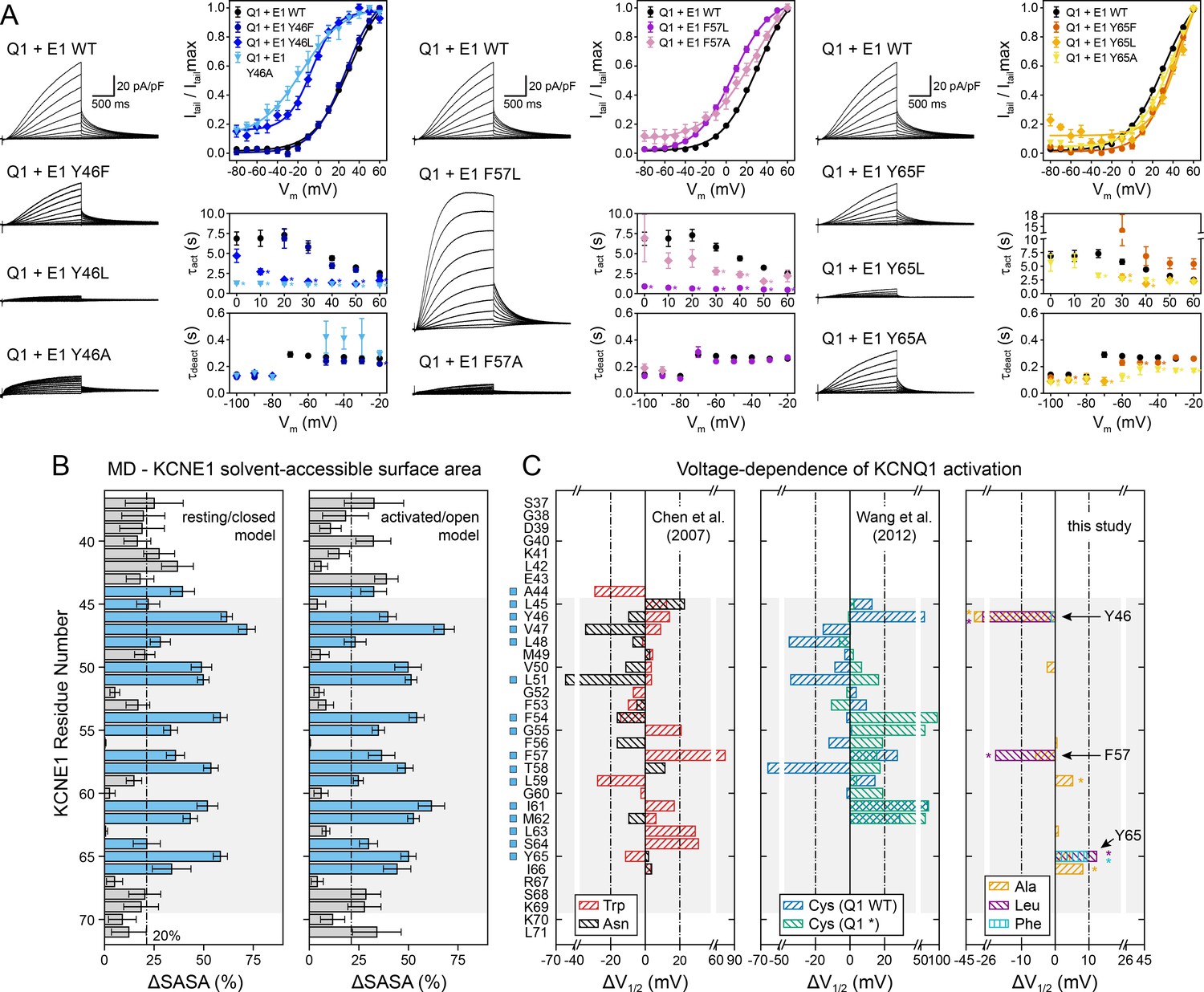
Experimental validation of KCNE1 TMD residues interacting with KCNQ1.
(A) Whole-cell currents measured from CHO-K1 cells transiently expressing KCNQ1 with KCNE1 WT or KCNE1 variants carrying mutations at residues Y46, F57, or Y65, respectively. Normalized activation curves are shown next to the currents (mean ± SEM, WT n = 270, Y46F n = 28, Y46L n = 14, Y46A n = 14, F57L n = 58, F57A n = 14, Y65F n = 23, Y65L n = 23, Y65A n = 18). Solid lines represent fits with a Boltzmann function (Itail/Itailmax = (1-IBottom) / (1+exp[(V1/2app-V)/k]) + IBottom) with the parameters of the fit summarized in Supplementary file 1 – Table 6. Activation time constants (τact) and deactivation time constants (τdeact) from fits to currents at each potential (WT n = 56–293, Y46F n = 8–36, Y46L n = 15–32, Y46A n = 22–30, F57L n = 58–66, F57A n = 3–17, Y65F n = 4–24, Y65L n = 17–57, Y65A n = 10–29). Time constants significantly different from those of WT KCNQ1+KCNE1 are indicated (*p<0.001, Student’s t-test). (B) Change in residual solvent-accessible surface area (ΔSASA) between KCNE1 alone and KCNE1+KCNQ1 calculated from MD simulations of the KCNQ1-KCNE1 RC and AO model (mean ± SD). ΔSASA values > 20% are shown with blue bars and indicate that a residue is part of the KCNQ1-KCNE1 interface. The approximate region of the KCNE1 TMD is indicated in gray. (C) Change in voltage-dependence of KCNQ1 activation by mutations in KCNE1. ΔV1/2 values of Trp and Asn mutants were previously reported by Chen and Goldstein, 2007, and those of Cys mutants are from Wang et al., 2012. In the latter case, experiments were performed with WT or Cys-less KCNQ1 (Q1*). Positions where mutations led to a significant change in V1/2 (|V1/2|>20 mV for KCNE1 expressed in oocytes in previous studies (Wang et al., 2012; Chen and Goldstein, 2007), |V1/2|>10 mV for KCNE1 expressed in CHO-K1 cells in this study) are indicated (■). (mean, *p<0.001, Student’s t-test).
-
Figure 7—source data 1
Excel file with numerical data used for panels A-C in Figure 7.
- https://cdn.elifesciences.org/articles/57680/elife-57680-fig7-data1-v1.xlsx
Figure 7—figure supplement 1
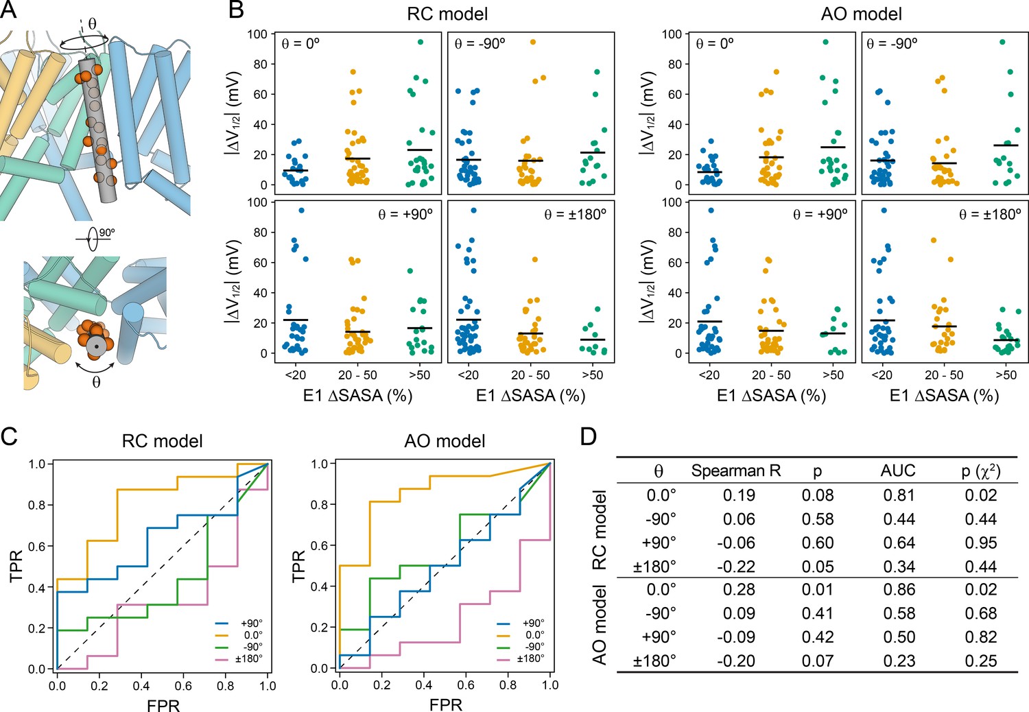
Comparison between the model-predicted KCNE1 TMD orientation and the pattern of V1/2 changes owing to mutations in KCNE1.
(A) Schematic showing the definition of the helical screw axis in KCNE1 and associated rotation angle θ. High-impact mutation sites in the KCNE1 TMD with |ΔV1/2| > |ΔV1/2|threshold (see Figure 7C) are shown as red spheres in the structural model. (B) KCNE1 residues are grouped according to their change in solvent-accessible surface area (ΔSASA) between KCNE1 alone and KCNE1 bound to KCNQ1, and their |ΔV1/2| values are plotted. The group average is indicated by a black line. The rank correlation between ΔSASA and |ΔV1/2| for the KCNE1 orientation predicted by the structural models in this work (θ = 0°) is compared to cases where KCNE1 is rotated 90° or 180° in the clockwise or anticlockwise direction. (C) Receiver operating characteristic (ROC) curves for classifying a KCNE1 position as high-impact mutation site based on its residue ΔSASA value. A ROC curve above the dashed line indicates that in this orientation residues with high ΔSASA value (i.e. KCNQ1-contacting residues) coincide with high-impact mutation sites better than with 50% chance. (D) Summary of the statistics computed for the classification tasks in (B) and (C) for the model-predicted and three other hypothetical KCNE1 helix orientations: Spearman rank correlation coefficient with associated p-value, area under the ROC curves (AUC), and p-value for the χ2 test of independence of the frequencies of KCNQ1-contacting and high-impact mutations sites using a ΔSASA cutoff of 20%.
-
Figure 7—figure supplement 1—source data 1
Excel file with numerical data used to make panels B-D of Figure 7—figure supplement 1.
- https://cdn.elifesciences.org/articles/57680/elife-57680-fig7-figsupp1-data1-v1.xlsx
Figure 8 with 1 supplement

Comparison of KCNQ1-KCNE1 models with structures of the KCNQ1-KCNE3 complex.
(A) Left: KCNE1 model bound to KCNQ1 in the RC conformation. Right: Experimental structure of KCNE3 (Sun and MacKinnon, 2020) bound to KCNQ1 in a decoupled state with an activated VSD and a closed PD (PDB: 6V00). KCNE1 residues Y46, F57, T58, L59, Y65, and the corresponding residues in KCNE3 are shown in spheres. (B) Left: KCNE1 model in complex with KCNQ1 in the AO conformation. Right: Experimental structure of KCNE3 (Sun and MacKinnon, 2020) bound to KCNQ1 with an activated VSD and an open PD (PDB: 6V01). (C) Residue neighborhood around Y46 in KCNE1 and its homologous residue Y60 in KCNE3. (D) Binding site of KCNE1 FTL and KCNE3 TVG. The putative H-bond between KCNQ1 Y267 and KCNE1 T58 is indicated by a dashed line. (E) Residue neighborhood around Y65 in KCNE1 and its homologous residue Y79 in KCNE3. (F) Occurrence of the Y267-T58 H-bond in MD simulations of the KCNQ1-KCNE1 RC and AO model.
-
Figure 8—source data 1
Excel file with MD H-bond time series data used for Figure 8 panel F.
- https://cdn.elifesciences.org/articles/57680/elife-57680-fig8-data1-v1.xlsx
Figure 8—figure supplement 1
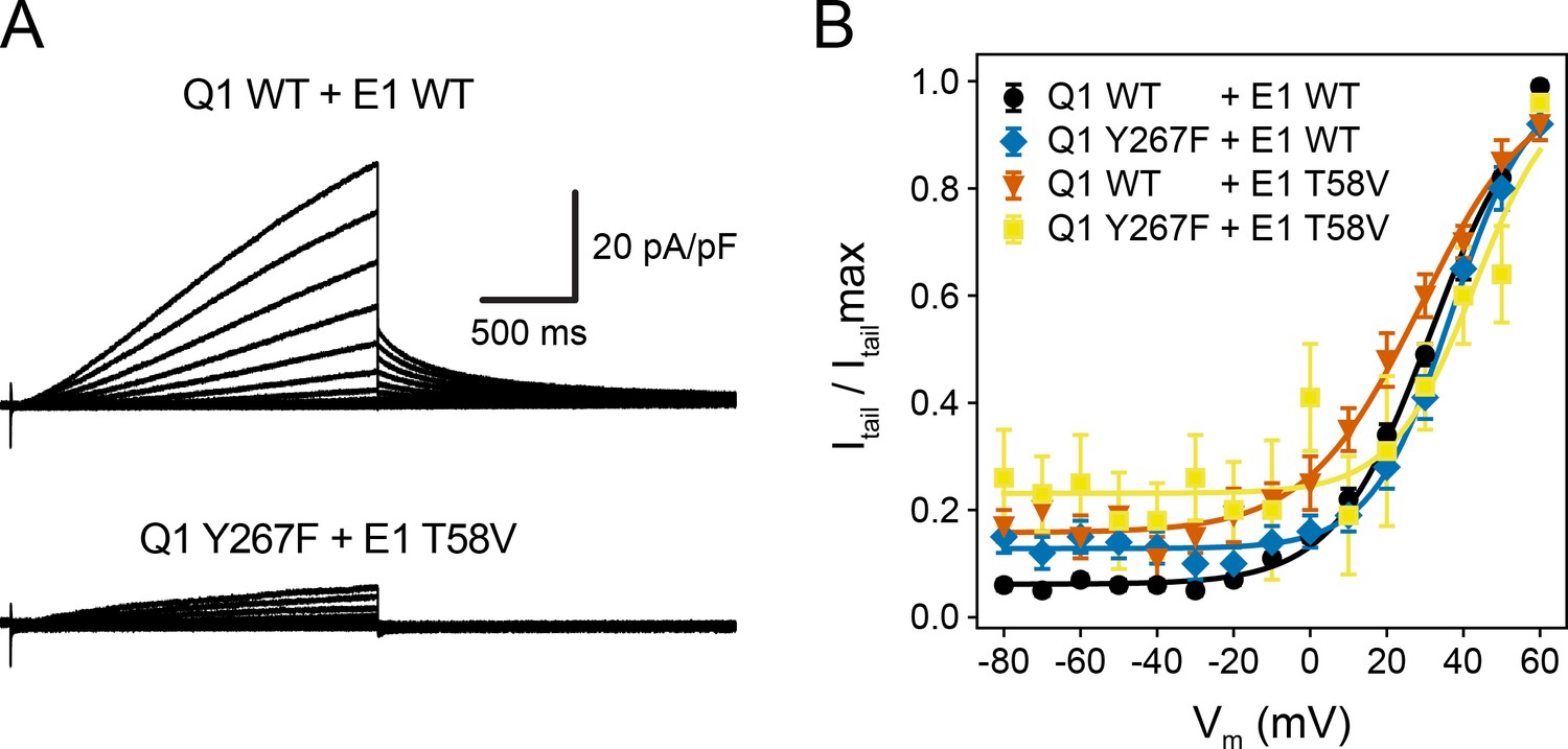
Double mutant cycle analysis for residue pair KCNQ1 Y267–KCNE1 T58.
(A) Whole-cell currents of wildtype KCNQ1-KCNE1 channel and KCNQ1 Y267F–KCNE1 T58V. (B) Normalized activation curves for KCNQ1-KCNE1, KCNQ1 Y267F–KCNE1, KCNQ1–KCNE1 T58V, and KCNQ1 Y267F–KCNE1 T58V. From Boltzmann function fits, the following free energy changes of channel opening were obtained: ΔGY267F = 0.66 kcal/mol, ΔGT58V = -0.36 kcal/mol, ΔGY267F/T58V = 0.90 kcal/mol. The coupling energy was calculated as ΔΔG = ΔGY267F/T58V – (ΔGY267F + ΔGT58V) = 0.60 kcal/mol. (mean ± SEM, WT/WT n = 70, Y267F/WT n = 32, WT/T58V n = 24, Y267F/T58V n = 11).
Figure 9 with 2 supplements
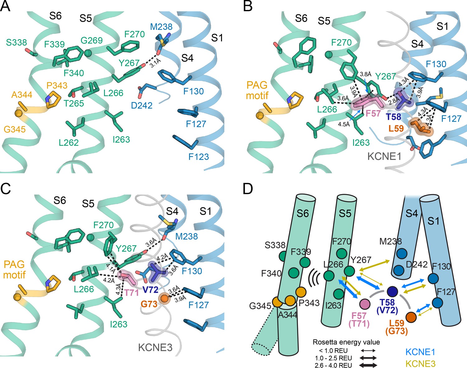
The activation motifs of KCNE1 and KCNE3 form distinct interactions with the VSD and PD that may induce different allosteric effects on S6.
(A) KCNE1/3 binding cleft in unbound KCNQ1 (PDB: 6UZZ) (Sun and MacKinnon, 2020). Residues on S1, S4, and S5, which surround FTL in the KCNQ1-KCNE1 model and TVG in the KCNQ1-KCNE3 structure, as well as residues in the S6 helix are shown. (B) Predicted binding mode of the KCNE1 FTL as discussed in the text. Potentially interacting residues are indicated and their distances are labeled. (C) Binding mode of the KCNE3 TVG observed in the KCNQ1-KCNE3 structure (PDB: 6V00). The distances to potentially interacting residues are labeled. (D) Schematic representation of the interactions induced by binding of KCNE1 (blue arrows) and KCNE3 (olive arrows), respectively. The expected relative strength of an interaction computed with the Rosetta energy function is indicated by the arrow thickness (Rosetta energy unit, REU). KCNE1/3 binding may be allosterically coupled to S6 as supported by previously reported functional interactions of KCNE3 with S338, and KCNE1 with F339 and F340 (Melman et al., 2004; Panaghie et al., 2006). Those interactions may affect S6 kinking at the PAG motif and influence gate opening.
Figure 9—figure supplement 1

Rosetta energy calculations and dynamical network analysis suggest that KCNQ1 S5 makes distinct interactions with KCNE1 and is part of a putative allosteric network connecting KCNE1 with KCNQ1 S6.
(A) Residue interaction networks calculated from MD simulations of the KCNQ1-KCNE1 RC (left) or AO model (right), respectively. Network edges between residues are drawn as solid lines. Smaller subnetworks (termed communities) partition the original network and are shown in different colors. Communities correspond to regions of the protein complex which move in a concerted fashion. Pathways in the network connecting KCNE1 T58 and KCNQ1 F340 are colored blue. The shortest path between T58 and F340 is shown in red. (B) Betweenness centrality (BC) of residues along pathways connecting T58 and F340 in the KCNQ1-KCNE1 RC (left) or AO model (right), respectively. Betweenness centrality corresponds to the number of shortest paths from all nodes to all others that pass through that residue. Thus, residues with higher betweenness are important for communication within the protein. Residues with high betweenness are in S5, S6, and KCNE1. (C) Rosetta interface scores (I_sc) for the interaction of KCNQ1 S5 with KCNE1 or KCNE3, respectively. Residues are colored according to their I_sc values (white: 0 REU, red: ≤−3.0 REU) (indicated in parentheses). (D) Computationally predicted changes of the interface score for KCNQ1-KCNE1 and KCNQ1-KCNE3, respectively, after substituting each S5 residue for alanine. Data represent the mean ± SEM interface score change of 30 independent Rosetta FlexddG (Barlow et al., 2018) calculations.
Figure 9—figure supplement 2
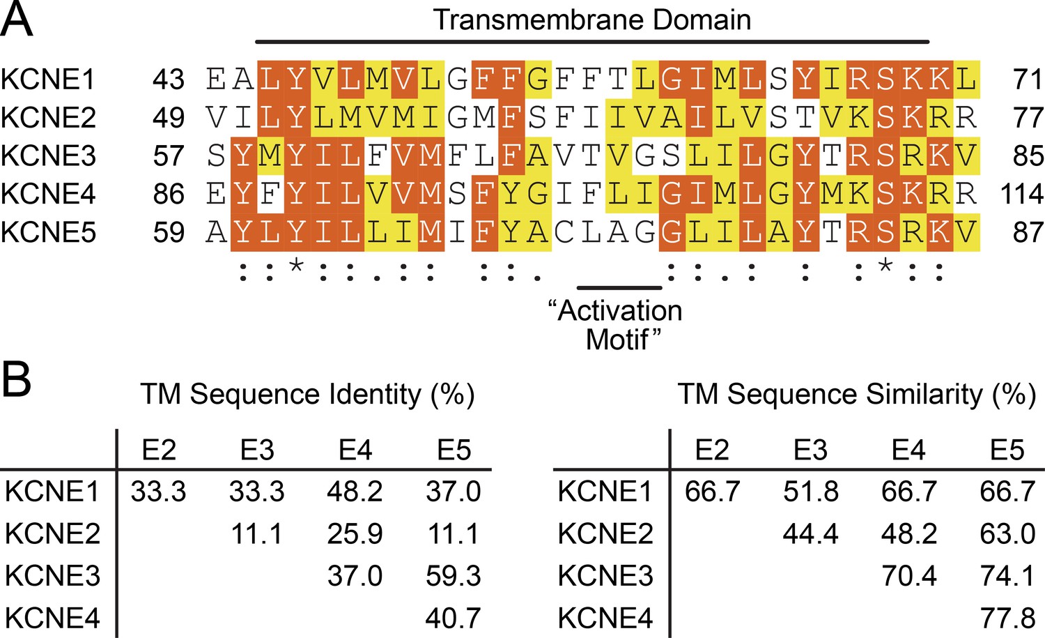
TMD sequence conservation within the KCNE family.
(A) Multiple sequence alignment of the TMD from KCNE1-5. Similar and identical amino acid residues are colored yellow and red, respectively. The position of the ‘activation motif’, which corresponds to FTL in KCNE1, is indicated. (B) Sequence identity and similarity calculated over the TM region in (A) between KCNE family members.
Author response image 1
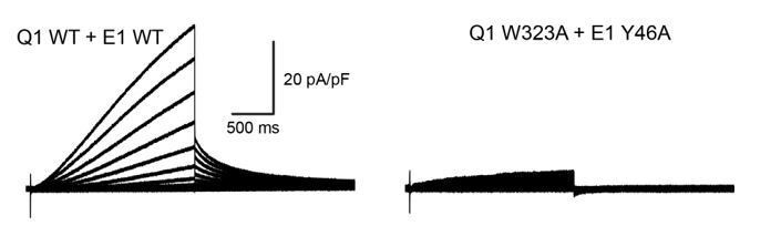
Whole-cell currents recorded from CHO-K1 cells expressing wildtype KCNQ1+KCNE1 (left) or KCNQ1 W323A+KCNE1 Y46A (right).
Author response image 2
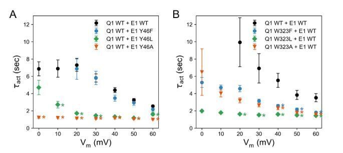
Activation time constants of channels formed with (A) KCNQ1 WT and KCNE1 Y46 mutants and (B) KCNQ1 W323 mutants and KCNE1 WT.
(mean ± SEM; * P < 0.001, Student’s t-test).
Author response image 3
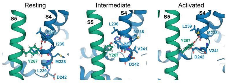
Interactions between Y267 and S4 in KCNQ1 models of the resting, intermediate, and activated state.
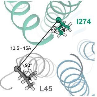
Author response image 4
Author response image 5

Whole-cell currents recorded from oocytes expressing KCNQ1_V141C + KCNE1_L45C treated with control bath solution and Cu-phenanthroline.
Videos
Video 1
Animation of KCNQ1-KCNE1 interaction sites in the KCNQ1-KCNE1 RC channel model.
Video 2
Animation of KCNQ1-KCNE1 interaction sites in the KCNQ1-KCNE1 AO channel model.
Video 3
Morph between KCNQ1-KCNE1 RC and AO models illustrating S6 helix kinking at the PAG motif during channel opening and the location of the KCNE1 FTL motif.
Video 4
Animation and comparison of the interaction sites of the activation motifs from KCNE1 and KCNE3.
Tables
Key resources table
| Reagent type (species) or resource | Designation | Source or reference | Identifiers | Additional information |
|---|---|---|---|---|
| Cell line (Cricetulus griseus) | CHO-K1 | ATCC Manassas, VA | RRID:SCR_001672 | Expression cell line |
| Gene (Homo sapiens) | KCNQ1 | HUGO Gene Nomenclature Committee (HGNC) | Gene ID: 3784; HGNC:629 | |
| Gene (Homo sapiens) | KCNE1 | HUGO Gene Nomenclature Committee (HGNC) | Gene ID: 3753; HGNC:624 | |
| Commercial assay, kit | Nucleobond Xtra Maxi EF | Macherey-Nagel Inc, Bethlehem, PA | Cat. # NC00089196 | Used to isolate DNA |
| Recombinant DNA reagent | pIRES2-EGFP | BD Biosciences-Clontech Mountain View, CA | Used to express KCNQ1 | |
| Recombinant DNA reagent | pIRES2-Scarlet | PMID:19687231 | Used to express KCNE1 | |
| Commercial assay, kit | QuikChange II XL | Agilent technologies Santa Clara, CA | Cat. # 200521 | Used to generate channel protein variants |
| Chemical compound, drug | Fugene six transfection reagent | Promega Corporation Madison, WI | Cat. # E2691 | Used to transfect cDNAs |
| Chemical compound, drug | JNJ 303 | TOCRIS Minneapolos, MN | Cat. # 3899 | Chemical compound, drug |
| Software, algorithm | Excel | Microsoft Redmon, WA | Data analysis | |
| Software, algorithm | PatchController | Nanion Technologies Munich, Gemany | Electrophysiology data collection | |
| Software, algorithm | DataController | Nanion Technologies Munich, Gemany | Electrophysiology data analysis | |
| Software, algorithm | Clampex | Axon Instruments Sunnyvale, CA | RRID:SCR_011323 | Electrophysiology data collection |
| Software, algorithm | Clampfit | Axon Instruments Sunnyvale, CA | RRID:SCR_011323 | Electrophysiology data analysis |
| Software, algorithm | Sigmaplot | SPSS San Jose, CA | RRID:SCR_003210 | Data plotting |
| Software, algorithm | GraphPad Prism | GraphPad Software San Diego, CA | RRID:SCR_000306 | Data analysis and plotting |
| Software, algorithm | ROSETTA (version 3.9) | PMID:21187238 URL: https://www.rosettacommons.org/ | RRID:SCR_015701 | Protein-protein docking |
| Software, algorithm | MolProbity | PMID:17452350 URL: http://molprobity.biochem.duke.edu | RRID:SCR_014226 | Analysis of docking models |
| Software, algorithm | CHARMM-GUI | PMID:25130509 URL: http://www.charmm-gui.org | Preparation of MD system | |
| Software, algorithm | AMBER 16 | PMID:16200636 URL: https://ambermd.org | RRID:SCR_014230 | Program for execution of MD simulations |
| Software, algorithm | CPPTRAJ | PMID:26583988 URL: https://ambermd.org/AmberTools.php | Tools for analysis of MD trajectories | |
| Software, algorithm | Antechamber | PMID:16458552 URL: https://ambermd.org/AmberTools.php | Parameterization of PIP2 lipid molecule | |
| Software, algorithm | Gaussian 09 | Gaussian, Inc, Wallingford CT URL: https://gaussian.com | RRID:SCR_014897 | Parameterization of PIP2 lipid molecule |
| Software, algorithm | PyMOL | The PyMOL Molecular Graphics System, Version 2.0 Schrödinger, LLC URL: https://pymol.org/ | RRID:SCR_000305 | Visualization of KCNQ1-KCNE1 models |
| Software, algorithm | VMD | PMID:8744570 URL: https://www.ks.uiuc.edu/Research/vmd/ | RRID:SCR_001820 | Visualization of MD simulations |
| Software, algorithm | HOLE | PMID:9195488 URL: http://www.holeprogram.org | Calculation of channel pore radius | |
| Software, algorithm | NACCESS | URL: http://wolf.bms.umist.ac.uk/naccess/ | SASA calculation | |
| Software, algorithm | NetworkView Plugin for VMD | PMID:22982572 URL: https://www.ks.uiuc.edu/Research/ vmd/plugins/networkview/ | Network analysis of MD simulations | |
| Software, algorithm | Anaconda | Anaconda Software Distribution. Computer software. Vers. 2–2.4.0. Anaconda, Inc URL: https://www.anaconda.com | Data plotting |
Additional files
-
Supplementary file 1
Table 1: Parameters from Boltzmann function fits of normalized activation curves of KCNQ1-KCNE1 WT and cysteine mutants which were used in crosslinking experiments.
Table 2: Distance restraints used in generation of the closed state KCNQ1-KCNE1 docking model. Table 3: Distance restraints used in generation of the open state KCNQ1-KCNE1 docking model. Table 4: MolProbity statistics for KCNQ1-KCNE1 Rosetta models. Table 5: KCNQ1-KCNE1 residue contacts observed in MD simulations of the KCNQ1-KCNE1 RC and AO channel models. Table 6: Biophysical properties of IKs channels formed with KCNQ1 or KCNE1 mutants.
- https://cdn.elifesciences.org/articles/57680/elife-57680-supp1-v1.docx
-
Supplementary file 2
PDB coordinates of the KCNQ1-KCNE1 RC (closed state) docking model.
- https://cdn.elifesciences.org/articles/57680/elife-57680-supp2-v1.zip
-
Supplementary file 3
PDB coordinates of the KCNQ1-KCNE1 AO (open state) docking model.
- https://cdn.elifesciences.org/articles/57680/elife-57680-supp3-v1.zip
-
Transparent reporting form
- https://cdn.elifesciences.org/articles/57680/elife-57680-transrepform-v1.pdf
Download links
A two-part list of links to download the article, or parts of the article, in various formats.
Downloads (link to download the article as PDF)
Open citations (links to open the citations from this article in various online reference manager services)
Cite this article (links to download the citations from this article in formats compatible with various reference manager tools)
Allosteric mechanism for KCNE1 modulation of KCNQ1 potassium channel activation
eLife 9:e57680.
https://doi.org/10.7554/eLife.57680


