Spatial readout of visual looming in the central brain of Drosophila
- Janelia Research Campus, Howard Hughes Medical Institute, United States
- Department of Experimental Psychology, University College London, United Kingdom
- Department of Biomedical Engineering, Cornell University, United States
- Department of Neurological Sciences, University of Vermont, United States
Figures
Figure 1 with 3 supplements

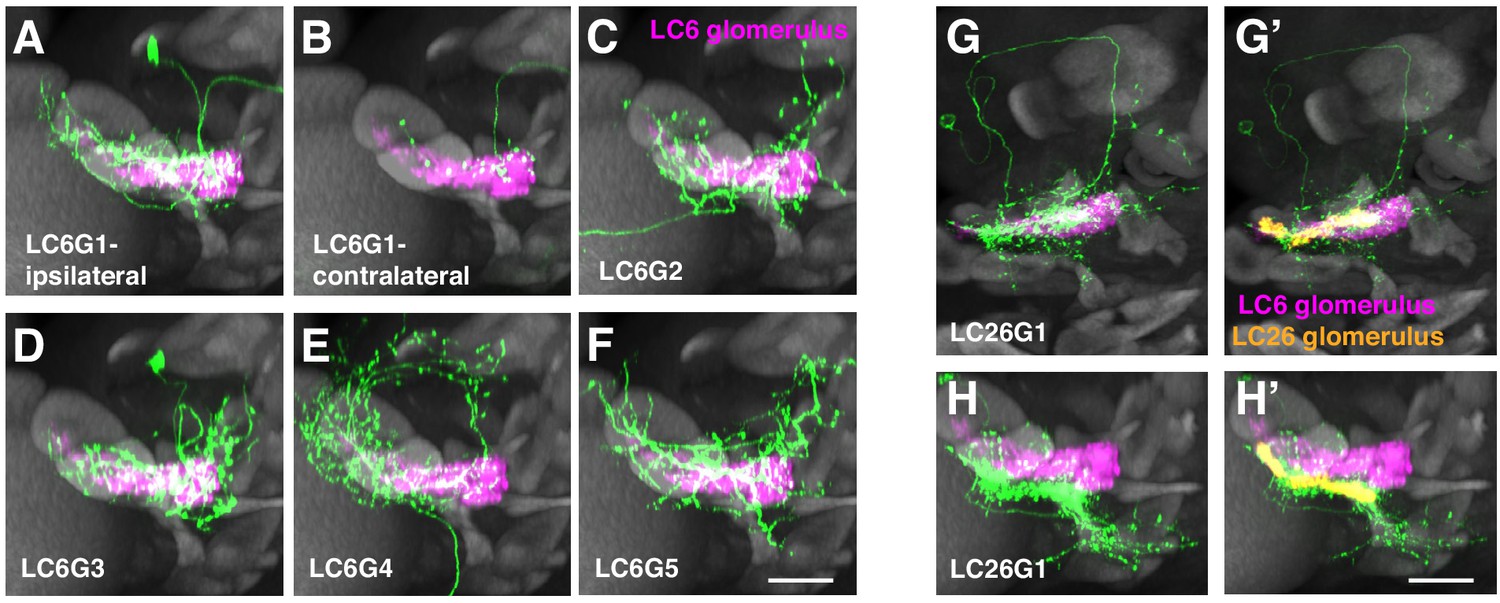
Multiple distinct cell types innervate the LC6 glomerulus.
(A–D) Projection pattern of LC6 neurons and (E–Q) anatomy of candidate LC6 target cells. All panels (except E), (F) show composites of registered confocal images together with the standard brain used for registration (shown in gray). To more clearly show the neurons of interest, some images were manually segmented to exclude additional labeled cells or background signal (see Materials and methods). (A) Lobula Columnar (LC) neurons project from the lobula to synapse-rich structures in the posterior ventrolateral protocerebrum (PVLP) called optic glomeruli. Two LC6 cells projecting to the LC6 glomerulus are illustrated. Schematic adapted from Wu et al., 2016. In all panels except for N-Q dorsal is up and medial is to the right. (B, C) LC6 neuron dendrites collectively tile the lobula, while the axons converge to form a glomerulus. (B, B’) Population of LC6 neurons labeled with a membrane targeted marker. Scale bar, 20 µm. (C, C’) MultiColor FlpOut (MCFO)-labeled individual LC6 cells registered and displayed as in (B). Note that individual LC6 terminals overlap in the LC6 glomerulus, while dendrites in the lobula occupy distinct positions. (D) Terminal of a single MCFO-labeled LC6 cell displayed as in (B’) with the LC6 glomerulus, based on the expression of syt-HA, a tagged synaptotagmin in LC6 cells as described in Wu et al., 2016, in magenta. (E, F) Examples of two populations of candidate LC6 target cells labeled by split-GAL4 driver lines. A membrane marker is in green, a synaptic marker (anti-Brp) in magenta. Scale bar, 50 µm. (G) MCFO labeling of two LC6G2 cells in the same specimen. (H–M) Examples of single cells of potential LC6 targets. All images show MCFO-labeled manually segmented single cells (green) together with the standard brain (gray) and LC6 glomerulus (magenta). Scale bar, 20 µm. (N–O) Several LC6 glomerulus interneurons project to the anterior ventrolateral protocerebrum (AVLP). The images show projections through a sub stack rotated around the mediolateral axis by 90° relative to the view shown in panels (A–M) with the reference brain neuropil marker (gray). (N) LC6 glomerulus (magenta) and approximate boundaries of the AVLP (dotted white line). (O, P) LC6G4 and LC6G2 populations, as labeled by split-GAL4 lines. In addition to the membrane label (green) and standard brain (gray) a presynaptic marker (syt-HA) is shown (magenta). Note syt-HA labeling in the AVLP. (Q) Overlay of the segmented single cells of LC6G2, LC6G3, LC6G4, and LC6G5 shown in (J–M) with the standard brain. Images in (N–Q) are sub stack projection, some cells in (O–Q) have additional AVLP branches outside of the projected volume. See Supplementary file 1 for detailed summary of fly lines used in this study.
Figure 1—figure supplement 1
Additional anatomical details of LC6G neurons.
(A–F) Views of the cells shown in Figure 1H–M rotated by 90° around the mediolateral axis. (G–H) Segmented LC26G1 cells displayed in the same views as the LC6G cells in Figure 1H–M (G, G’) and (A–F) (H, H’). The LC26 glomerulus outline is based on syt-HA expression in LC26 driven by an LC26 split-GAL4 driver (Wu et al., 2016). Note that LC26G1 shows only minor overlap with the LC6 glomerulus. Scale bar, 20 µm.
Figure 1—figure supplement 2

Expression patterns of LC6G split-GAL4 lines.
Maximum intensity projections through confocal stacks of brains immunolabeled for a GAL4-driven membrane marker (green) and a reference label (anti-Brp, magenta). Imaging parameters and post-imaging adjustments of brightness and contrast are not identical for different images. Scale bar, 50 µm. The line name and expressed cell type for each split-GAL4 line is indicated in the lower right corner. See Supplementary file 1 for detailed summary of driver lines used in this study.
Figure 1—figure supplement 3
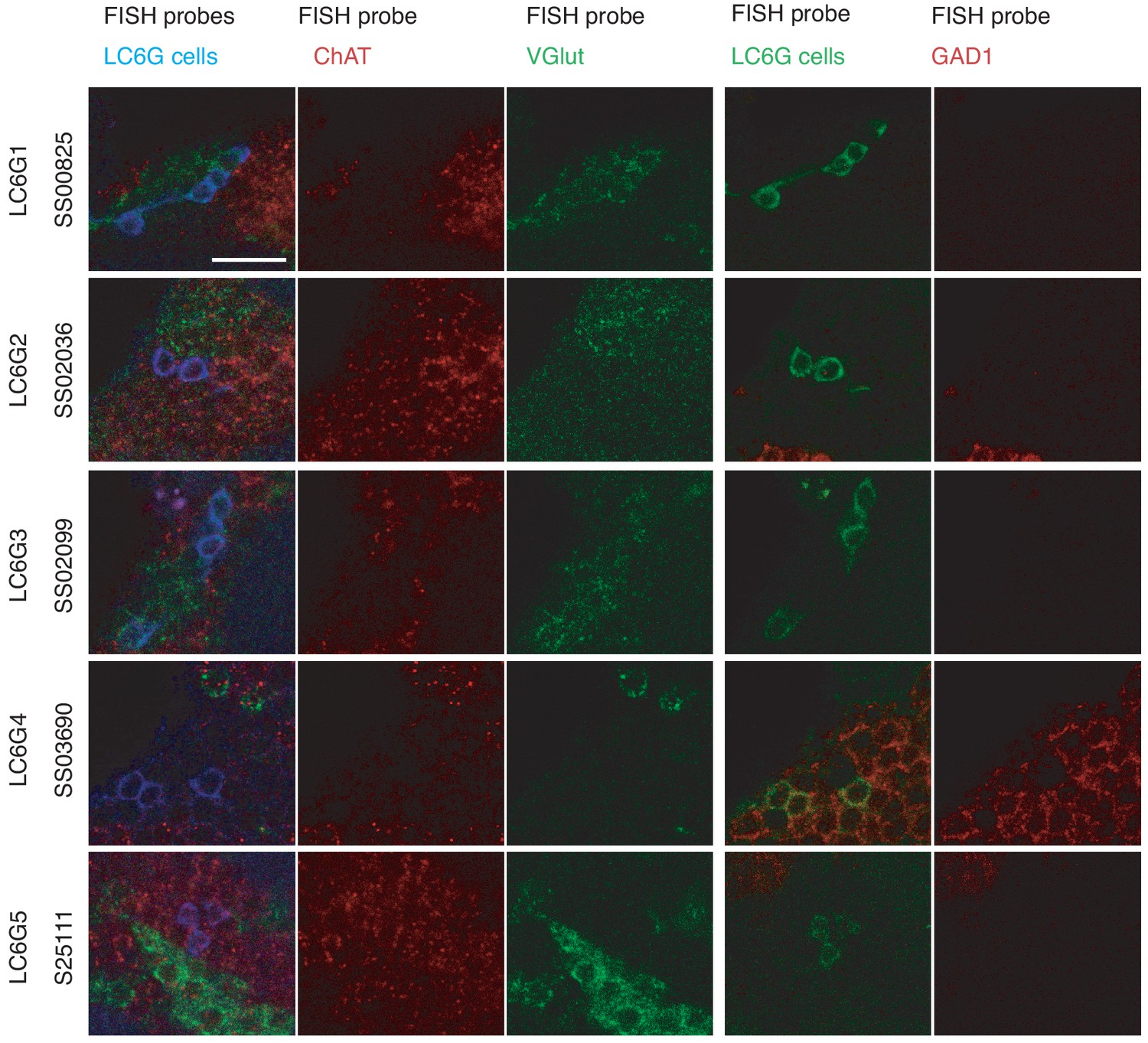
FISH detection of neurotransmitter markers in LC6G neurons.
Transcripts of GAD1, VGlut, and ChaT were detected by FISH as described in Meissner et al., 2019. Images show single slices of confocal stacks. Images for each driver line show the same group of cells but were acquired in two sets. The first and fourth columns are composites with the colors labeled along the top row indicating each probe. Cell bodies of cells with the same neurotransmitter phenotype are often found in groups (presumably from the same lineage). For example, both LC6G1 and LC6G3 cells are part of the same cluster of apparently glutamatergic neurons. Scale bar, 10 µm.
Figure 2 with 1 supplement
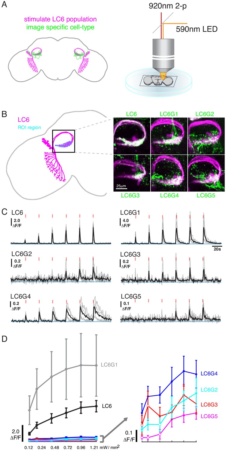
Pairwise functional connectivity reveals connected downstream cell-types.
(A) Chrimson was expressed in LC6 (magenta) using a LexA line, and GCaMP6f was expressed in individual candidate downstream neuron types or LC6 itself (green) using split-GAL4 lines. Chrimson was activated by pulses of 590 nm light, while GCaMP responses were imaged using two-photon microscopy. (B) Calcium responses were measured in the ROI region in cyan. Representative images of double-labeled (Chrimson in magenta, GCaMP6f in green) brains used for the experiment. (C) Calcium responses in candidate downstream neurons in response to LC6 Chrimson activation (N = 4–5 per combination; individual sample response in gray, mean response in black). A range of response amplitudes and timecourses were observed. Red tick marks indicate the activation stimulus. (D) Peak responses (mean ± SEM) are shown for each candidate downstream cell type for increasing light stimulation. Closed circles denote data points significantly different from pre-stimulus baseline, open circles denote data points not significantly different from pre-stimulus baseline (p<0.1, two-sample t-test). See Supplementary file 1 for detailed summary of fly lines used in this study.
Figure 2—figure supplement 1
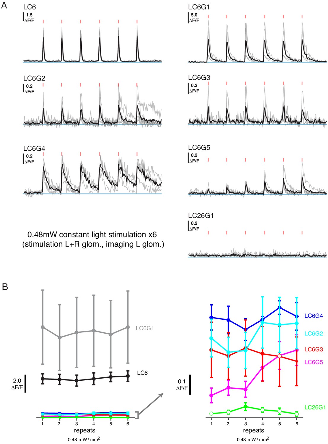
Additional functional connectivity results with alternative stimulation protocol and an additional cell type.
(A) Calcium responses of candidate downstream neuron types in response to LC6 Chrimson activation (N = 4–5 per combination; same flies as in Figure 2; individual mean sample response in gray, mean response across flies in black). Red tick marks indicate the activation stimulus. In this protocol, a constant illumination level was used for each stimulation repeat. (B) Peak response means (± SEM) are shown for each candidate downstream cell-type. Closed circles denote data points significantly different from pre-stimulus baseline, while open circles denote data points not significantly different from pre-stimulus baseline (p<0.1, two sample T-test). See Supplementary file 1 for detailed summary of driver lines used in this study.
Figure 3 with 3 supplements

Neurons downstream of LC6 exhibit stereotyped spatial receptive fields.
(A) Left: Schematic of the in vivo two-photon calcium imaging setup. An LED display was used to deliver looming stimuli at many positions around the fly, while calcium responses were measured from an ROI containing the LC6 glomerulus. Middle: Example stimulus time course and response of an LC6G2 neuron. Right: Small looming stimuli were delivered at 98 positions centered on a grid (and subtending ~ 18° diameter at maximum size) to map the receptive fields of LC6G neurons. (B, C) The bilateral LC6G1 and ipsilateral LC6G2 neurons showed consistent visual responses. LC6G1 responded throughout most of the stimulated area, with strongest responses near the equator and toward the midline, and LC6G2 responded within a more restricted receptive field. Gray-shaded regions indicate portions of the display that should not be visible to the fly. (B) Single animal example responses (from groups of ~ 4 cells of each LC6G neuron type), with each time series showing the mean of three repetitions of the stimulus at each location. The responses are plotted to represent the grid of looming stimuli mapped onto fly eye centered spherical coordinates (see Figure 3—figure supplement 1B; lines indicating the eye’s equator, frontal midline, and lateral 90°, are shown in gray). The (0,0) origin of each time series is plotted at the spatial position of the center of each looming stimulus (this alignment onto eye coordinates accounts for e.g. the upward curving stimulus responses below the eye equator). The 60% of peak response is demarcated with a contour (based on interpolated mean responses at each location). (C) The mean responses across multiple animals are shown (N = 4 for LC6G1, N = 7 for LC6G2), with the 60% of peak contours shown in a separate color for each individual fly. The responses have been normalized for each fly before averaging (detailed in Methods). Responses at each position that are significantly larger than zero are in black, others in gray (one-sample t-test, p<0.05, controlled for False Discovery Rate Benjamini and Hochberg, 1995). The individual responses are shown in Figure 3—figure supplements 1 and 2; the gray area indicates the region of the visual display that was occluded by the head mount (Figure 3—figure supplement 1B). See Supplementary file 1 for detailed summary of fly lines used in this study and Supplementary file 2 for summary of all visual stimuli presented.
Figure 3—figure supplement 1
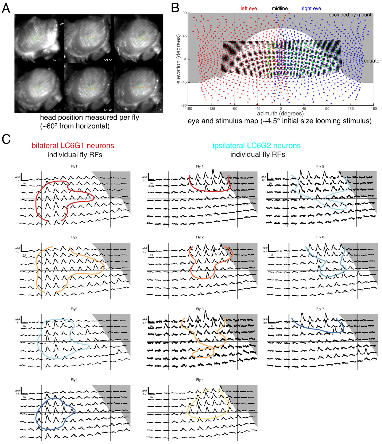
Eye map and individual fly receptive fields.
(A) Side view of head fixed fly. The ommatidial axes were used to determine the inclination of the head. Great care was taken to consistently align the fly head across preparations. (B) Overlay of ommatidial and stimulus maps in visual space coordinates. The extent of visual stimulation panels is shown as the black dots, each representing a single LED of the 32 × 96 array, and the green disc represents the center positions of each small looming stimulus used for RF mapping. Gray background areas were estimated to not be visible to the fly, from occlusion by head mount. (C) Calcium responses of LC6G1 and LC6G2 neurons, measured from individual flies, to the RF mapping stimuli (Figure 3A) Plotting conventions follow Figure 3B, and the colors for individual flies are carried over from Figure 3C. The accuracy of our alignment between individual flies and our visual stimulus is confirmed by the lack of visual responses for the occluded positions in the upper right corner (in gray). See Supplementary file 1 for detailed summary of driver lines used in this study.
Figure 3—figure supplement 2
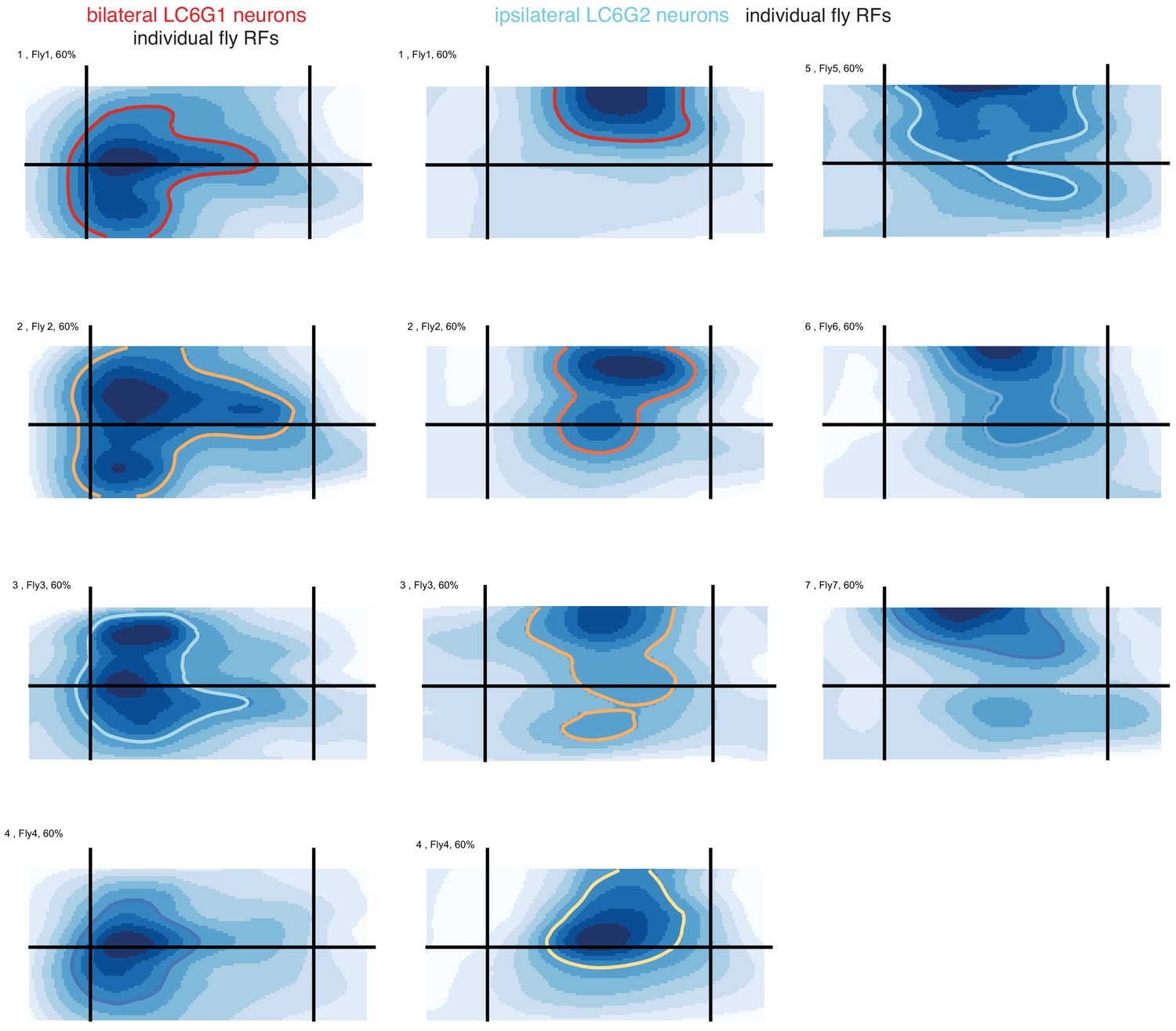
Receptive fields measured from individual flies, replotted as a heat map.
Same as in Figure 3—figure supplement 1C, but here replotted as a heat map, for comparison with Figure 7.
Figure 3—figure supplement 3
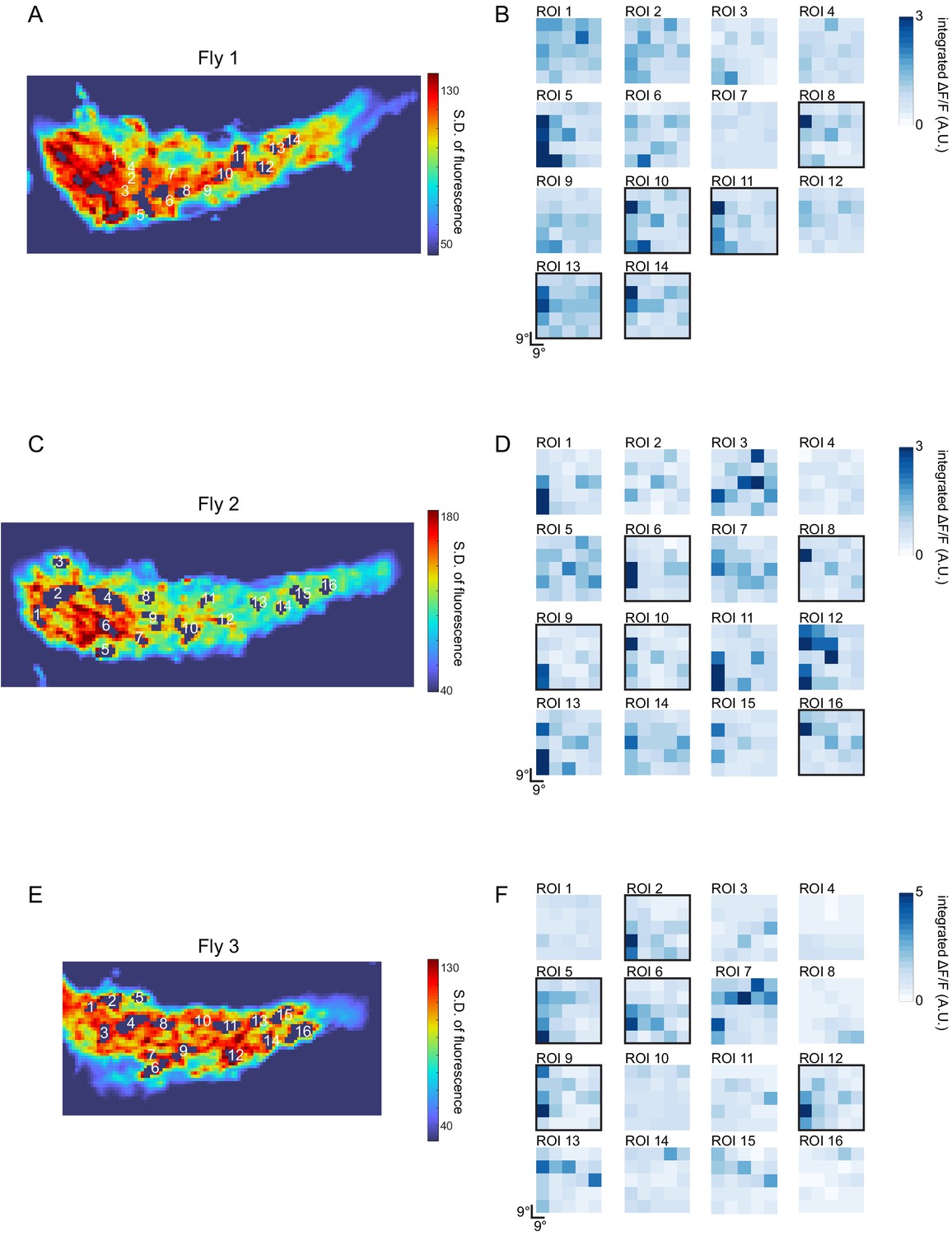
Estimation of LC6 receptive field size from GCaMP imaging of putative LC6 boutons in the glomerulus.
The responses of LC6 neurons to dark flashing squares (9°×9°) that were presented in a randomized order (on a grid spanning ~ 45° ×~45°, displayed from ~ 4.5° to ~ 49.5° from the eye’s (anterior) midline in azimuth and from the equator in elevation). Putative LC6 boutons were selected (as Regions of Interest, ROIs) using a threshold in the standard deviation of the pixel intensity over the entire stimulus presentation period (most active pixels shown in A, C, E; responses from three flies). Because the glomerulus is densely packed with LC6 axons, some pixels are expected to contain signals from more than one LC6 neurons. B, D, F show the spatial response profile (an approximate RF map) for each numbered ROI, generated by using the integrated calcium response during the 3, 3 s long trials. Approximately 30% of these putative LC6 spatial maps show focal responses (outlined with a black box). This suggests that the effective Receptive Field (as determined by this stimulus) of a single LC6 has a diameter of not more than ~ 20°.
Figure 4
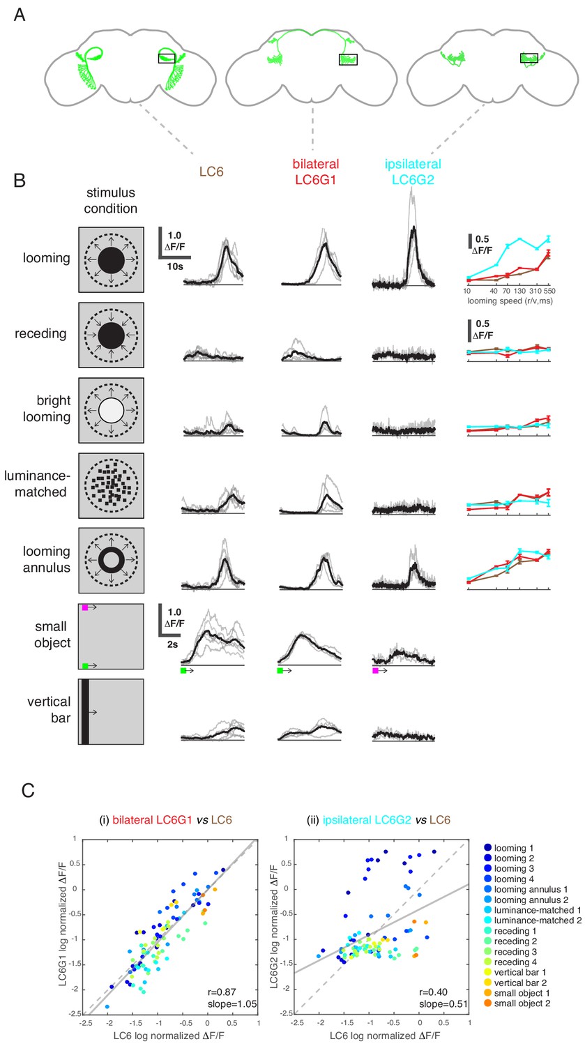
LC6 downstream neurons differentially encode visual stimuli.
(A) Schematic of LC6, bilateral (LC6G1), and ipsilateral (LC6G2) projecting downstream cell types. Black rectangles indicate the ROI selected for GCaMP imaging; visual stimuli were presented to the ipsilateral eye. (B) The calcium responses in LC6 and downstream neurons evoked by visual stimuli indicated by ‘stimulus condition.’ Times series are shown for the lowest speed (r/v = 550) in each stimulus category. The small object and vertical bar stimuli moved at 10°/s. Individual fly responses are in gray, and mean responses in black (LC6 N = 6, LC6G1 N = 4, LC6G2 N = 3). The tuning curves show peak responses for each speed of the looming and looming-related stimuli (mean ± SEM). Note that ‘luminance-matched’ stimulus does not contain looming motion, but the overall luminance was matched, frame-by- frame, to the looming stimulus at each speed tested. (C) Comparison between LC6 and the LC6G visual responses. LC6 and LC6G peak responses are log normalized and plotted against each other. LC6G1 (bilaterally projecting downstream) responses correlate well with that of LC6 (Pearson’s correlation, slope = 1.05, r = 0.87, p=5.7 × 10⁻²⁹), while LC6G2 (ipsilaterally projecting downstream) are not as well correlated (slope = 0.51, r = 0.40, p=7.7 × 10⁻⁵). Note that most of the looming responses are above the (X = Y) identity line, while most of the non-looming responses are below it, demonstrating enhanced selectivity for looming stimuli. Linear fit is in solid gray line, while the identity line is in dashed gray. The data points are color coded by visual stimulus condition (detailed in Materials and methods and Supplementary file 2). See Supplementary file 1 for detailed summary of fly lines used in this study and Supplementary file 2 for summary of all visual stimuli presented.
Figure 5 with 2 supplements
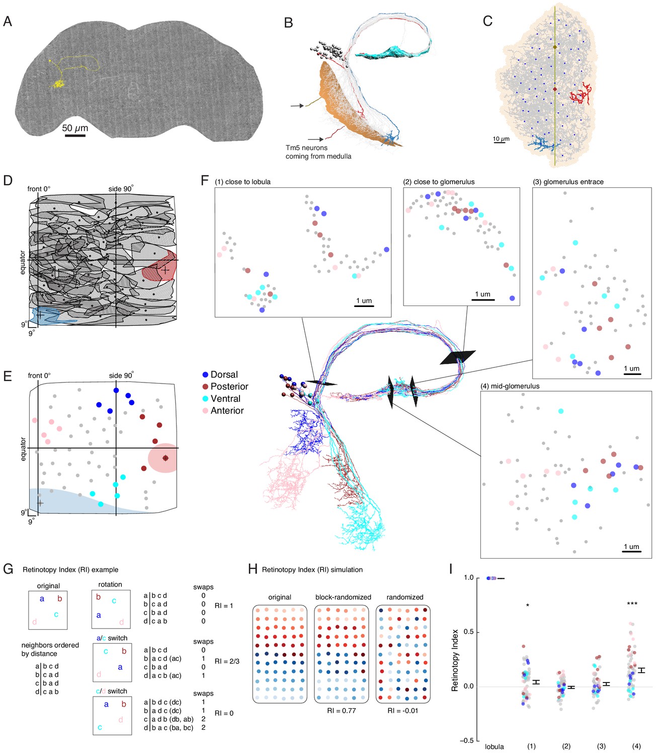
EM reconstruction of LC6 neurons connecting the optic lobe and the central brain.
(A) An example LC6 neuron found in Serial Section Transmission Electron Microscopy volume of the complete female brain. (B) All LC6 neurons on one side of the brain (by convention, the right side, but displayed here on left) were traced into the glomerulus. Two example cells are highlighted in red and blue (same cells in C, D, and E). All cells have dendrites mainly in lobula layer 4 (orange), and project to the LC6 glomerulus (cyan). Cell bodies are rendered as gray spheres. The projections of two Tm5 neurons are shown coming from the medulla side of the lobula. They were selected to identify the center (brown Tm5) and central meridian (both Tm5s) of the eye in C. (C) Projection view of the lobula layer. Traced LC6 dendrites (gray) are projected onto a surface fit through all dendrites (light orange). Blue disks represent centers-of-mass of each LC6 dendrites. The vertical line is the estimated central meridian, the line that partitions the eye between anterior and posterior halves, mapped onto the eye coordinate in D. (D) Estimate of dendritic field coverage of visual space (basis for anatomical receptive fields) for all LC6 neurons. Polygons are the estimated visual fields, and the boundary indicates the estimated boundary of the lobula (layer 4). The red example cell RF corresponds to posterior-viewing parts of the eye while the blue example cell RF corresponds to fronto-ventral viewing direction. In agreement with previous characterization of LC6 neurons (Wu et al., 2016), the dendrites appear to cover the entire visual field with significant overlap. This overlap is most prominent in the region of the lobula corresponding to the fronto-ventral part of the eye. Note that the central meridian is not shown in D and is not exactly the same as the line indicated by ‘side 90°’. (E) Four groups of five LC6 neurons, corresponding to different regions of visual space, used for exploring retinotopy in F. The filled regions are examples of the anatomical receptive field estimates, for the red and blue neurons in (B), (C), and (D). (F) Central figure shows the skeletons of the four groups of LC6 neurons with four cross-sections: (1) outside the lobula, (2) before the entrance of the glomerulus and (3 , 4) within the glomerulus. The disks in the four cross-section plots represent LC6 axons with the same color code as in (E). The positions of these axons show significant mixing, and do not generally mark the boundary of the group of neurons, as they do in the Lobula. The gray dots correspond to the 45 LC6 neurons not identified by one of the four groups; for compactness of this visualization, up to one gray dot per panel is omitted. (G) An example illustrating the Retinotopy Index, RI, that quantifies the amount of rearrangement occurring when a set of points is mapped from one space to another. On the left side is an example for four points, in the original space (such as the lobula), below is the (Euclidean) distance-based ranking of the points, using each point as a reference. In the middle are example transformations and the resulting distance-ranked lists. As detailed in the text and in the Materials and methods, the quantification is based on counting the number of swaps required to re-order the transformed list of points back to the original list. The RI for a point set and mapping is the averaged RI over all reference points. For mappings that preserve the order, the RI will be close to 1, while RI ~ 0, corresponds to (on average) a random mapping of the points (and therefore a random re-ordering of retinotopy). (H) Simulated examples of 2 mappings applied to a (jittered) grid of 66 points. In the first example (‘block-randomized’), the mapping maintains most of the global organization, but within the local blocks, the order has been randomized, resulting in an RI that is close to, but reduced from 1. In the second example, the order of the points has been completely randomized and the resulting RI for this mapping is ~ 0. (I) Retinotopy Indices for all 65 LC6 neurons (shown as individual points) at four cross-sections defined in (F) (plotted with their corresponding colors), with the lobula being the original space (RI = 1 at that location). The black dot and horizontal bars denote the mean ± SEM. Asterisks represent the result of the Mann-Whitney U test, comparing the population to 0; *p<0.05, ***p<0.001.
Figure 5—figure supplement 1

Distribution of LC6 arbors in the lobula from EM data.
Figure 5—figure supplement 2
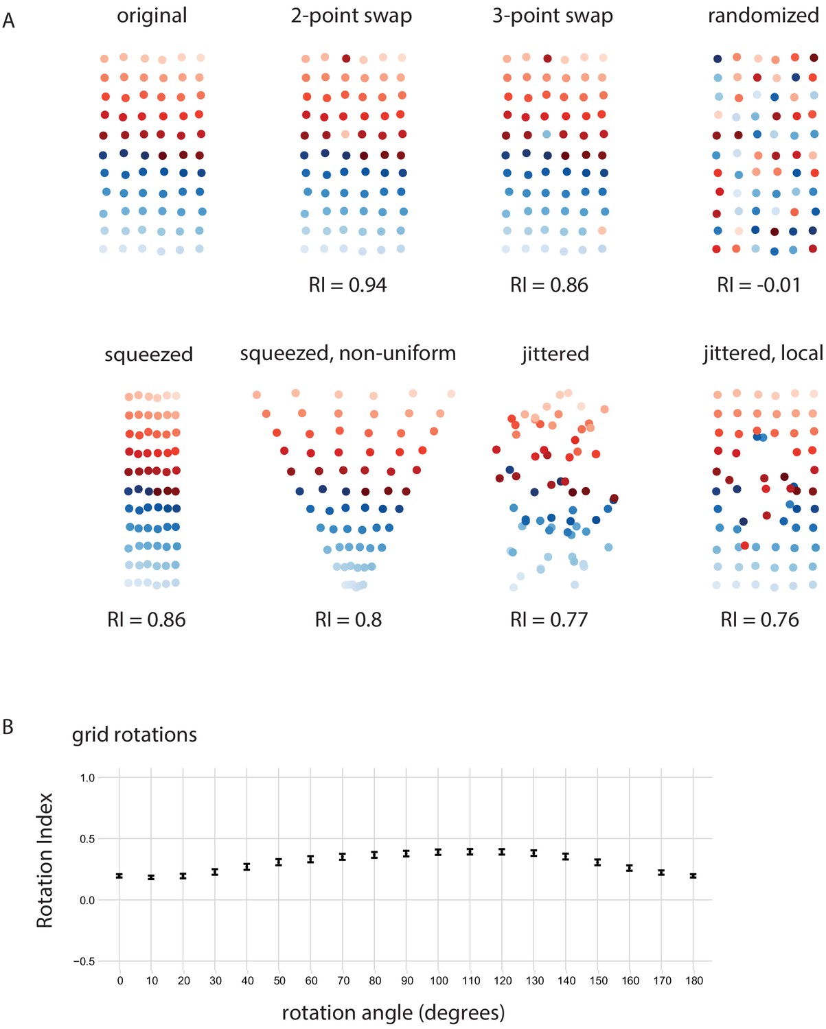
Retinotopy Index for simulated examples.
(A) Using 66 points that form an 11 × 6 grid(positions slightly jittered) as the ‘original’ point set, we consider several mappings to illustrate the Retinotopy Index (same set of points as in Figure 5H). Swapping 2 or 3 points leads to reductions from the maximal RI = 1, while a complete identity randomization results in an RI that is ~ 0. Squeezing the grid along one dimension (uniformly or non-uniformly) also leads to a reduction in the RI, because the proximity of the points is changed such that some points are now closer than others in the new space than they were in the original space. Jittering the points also leads to a reduction in RI. (B) The RI for projection onto a 1D line space after a rotation, similar to Figure 6E and F. The x-axis is the angle of rotation of the original point set, after which it is projected onto the x-axis and the RI is calculated.
Figure 6 with 1 supplement
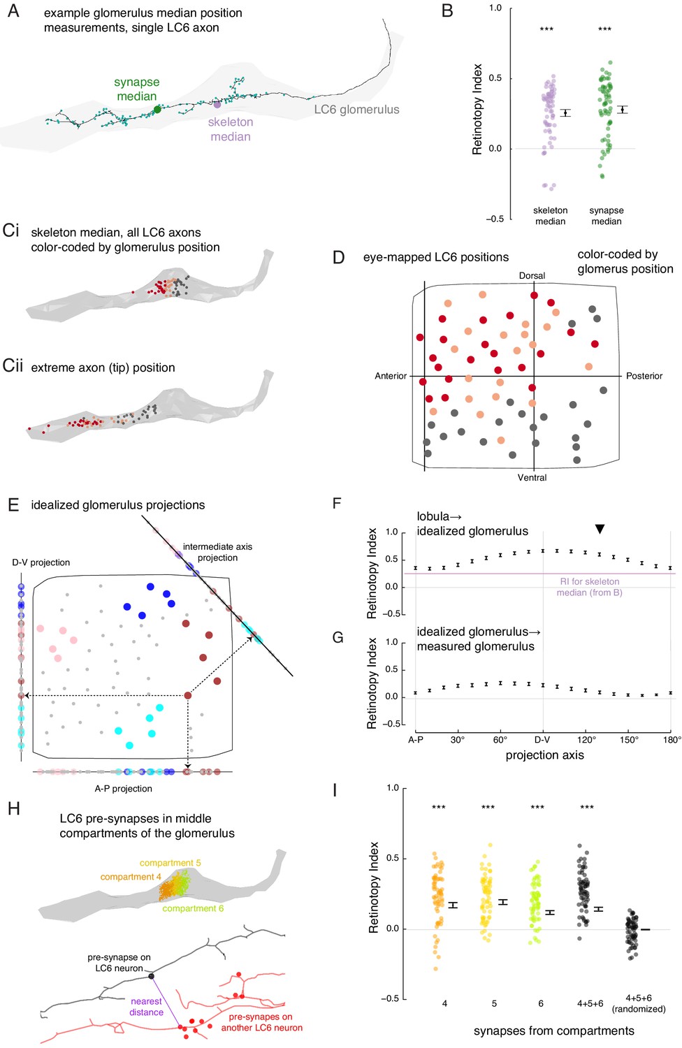
The organization of LC6 axons and their synapses in the glomerulus.
(A) An example of an LC6 axon within the glomerulus (in gray), with pre-synaptic sites indicated as cyan dots. The purple disc represents the median position of the skeleton while the green disc represents the median position of the pre-synapses (all positions first projected onto the long axis of the glomerulus). (B) Retinotopy Index for the mappings from lobula (as in Figure 5D) to the skeleton median and synapse median positions (summary is mean ± SEM). Asterisks represent the result of the Mann-Whitney U test, comparing the population to 0; ***p<0.001; plotting conventions as in Figure 5I. (Ci) LC6 skeleton median positions (illustrated in A) partitioned into three groups based on position on the long axis of the glomerulus (in gray). (Cii) The axon tip positions (the average position of the 10% of the nodes farthest from the glomerulus), color-coded based on the groups in Ci, reveal that the small differences in axon median positions reflect differences in the length of the axon. (D) LC6 dendrite center-of-mass in the visual field (based on Figure 5D) color-coded by their median position in the glomerulus (Ci). (E) As a comparison for the observed lobula-to-glomerulus position mapping, we construct a synthetic mapping as the projection from the 2D lobula space onto a 1D line-space, the 'idealized glomerulus', which is swept through a range of angles. Three example 1D line-spaces are shown along with the projection of the set of points representing the LCs onto each line; neurons are color-coded as in Figure 5E to help illustrate the transformation. (F) The Retinotopy Index (mean ± SEM) for the synthetic mapping from the lobula to the idealized glomerulus. The three line-spaces shown in E are labeled with ‘A-P’, ‘D-V’ and the intermediate axis is indicated with a black triangle. The mean RI corresponding to the skeleton median (from B) is reproduced. (G) The Retinotopy Index for mappings from the idealized glomerulus line-spaces to the skeleton median in the glomerulus. (H) Three compartments in the middle of the glomerulus, selected since they contain synapses of all LC6 neurons; the colored dots show the position of the pre-synapses on all LC6 neurons in each compartment (Figure 6—figure supplement 1B). Below is an example illustrating the key step in a synapse-based definition of distance: the minimal distance between a pre-synapse on one LC6 neuron and the set of pre-synapses on a second LC6 neuron. See Materials and methods for details. (I) The Retinotopy Index (summary is mean ± SEM) for comparing the synapse-based distance of the LC6 neurons to their ordering in the lobula, for each of the three compartments in H, all three compartments combined, and combined then identity-randomized. Asterisks represent the result of the Mann-Whitney U test, comparing the population to 0; ***p<0.001; plotting conventions as in Figure 5I.
Figure 6—figure supplement 1
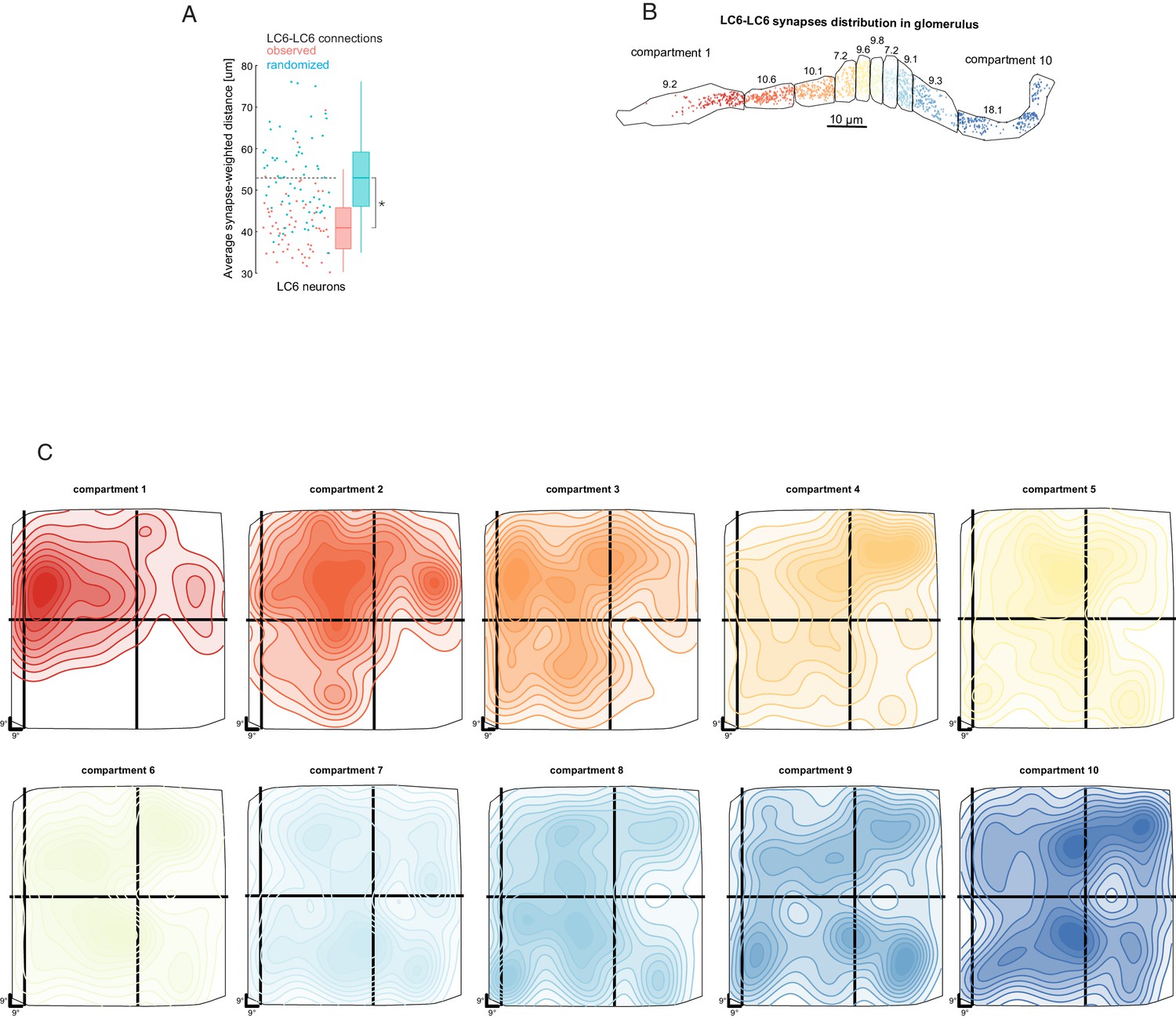
Biased connectivity and visual sampling by LC6 synapses in the glomerulus.
(A) Analysis of LC6-LC6 connections in the glomerulus. LC6 neurons contact their dendritic neighbors with significantly greater probability than chance (shuffled for same number of synapses, but with visual-spatial relationships scrambled; Mann-Whitney U test, p=~0.015). The synapse-weighted distance is calculated by summing the products of distance and number of synapses between a given LC6 and the all others and the dividing by the total number of incoming synapses. (B) LC6-presynapes within 10 compartments of the glomerulus, selected to contain an equal number of LC6 pre-synapses. The numbers are the percentage of LC6-LC6 synapses within each compartment. (C) 10-level contour plots of the LC6-LC6 synapse-weighted spatial receptive field for each compartment (colors matched to B) plotted in the coordinates of the field of view of one eye. The general trend is for middle compartments to reflect broader spatial distribution, while compartments 1, 2, and 3 exhibit an anterior-dorsal bias (consistent with Figure 6C,D).
Figure 7 with 3 supplements

Connectivity-based readout of visual information in the LC6 glomerulus corroborates features of the spatially selective responses of target neurons.
(A) Bilaterally projecting LC6G1 and ipsilaterally projecting LC6G2 neurons were identified and reconstructed in the full brain EM volume. Individual neurons shown in Figure 7—figure supplement 1. (B) Summary connectivity matrix of LC6, LC6G1, and LC6G2 neurons, each cell type is grouped, with the side of the brain (R or L) and the number of neurons in each group labeled. See Supplementary file 3 for the complete connectivity matrix. (C) Estimated anatomical RFs of each target neuron type. Each LC6 neuron’s RF is scaled by the number of synapses to each individual target neuron, and then summed across all neurons of the same type (see Materials and methods for details). RFs for each individual target neuron shown in Figure 7—figure supplement 1. The 70% contour is highlighted with a dark blue line. (D) Anatomical RF (blue contour) overlaid onto functional RF measured in vivo (replotted from Figure 3C, but with the average 60% of peak contour shown here). Further comparisons between these cell types and between EM and functional estimates of the RFs are in Figure 7—figure supplements 2 and 3.
Figure 7—figure supplement 1
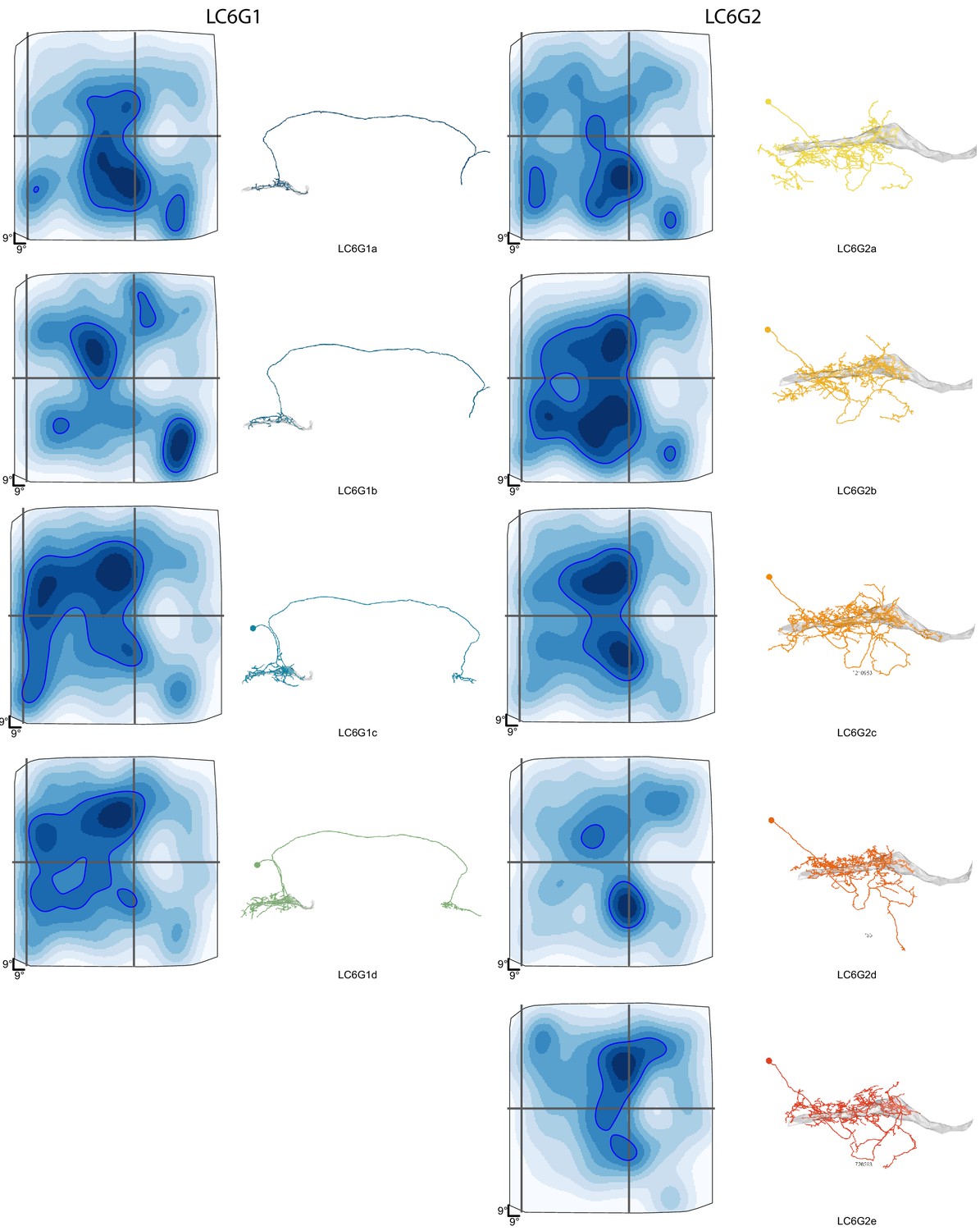
Details of reconstructed LC6G neuron morphology and estimated anatomical Receptive Fields.
An overview of the morphology and estimated anatomical Receptive Field for each LC6G neurons. The individual neurons are named by the type and a letter code. These individual neuron names are used in Figure 7—figure supplements 2 and 3.
Figure 7—figure supplement 2
Organization of downstream target neurons in the glomerulus.
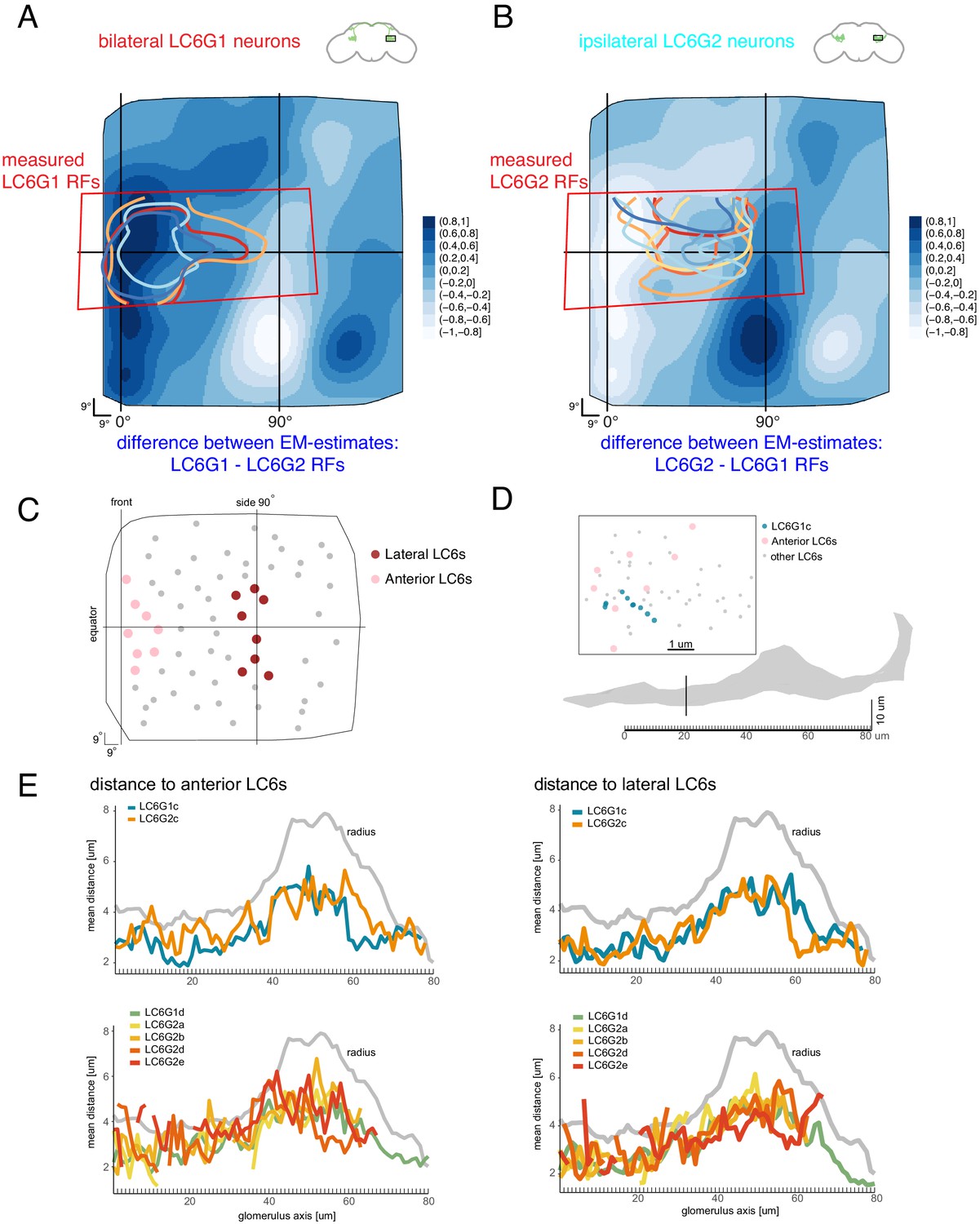
The difference between the anatomy-based RFs estimates from Figure 7D are plotted to compare the functional measurements with the differences between the anatomical estimates. (A) LC6G1 - LC6G2 anatomical RFs, overlaid with the measured LC6G1 RF (individual lines correspond to measurements from individual flies, from Figure 3). (B) LC6G2 - LC6G1 anatomical RFs, overlaid with the measured LC6G2 RF (from Figure 3). (C) The selection of eight anterior and eight lateral LC6s. (D) The distribution of LC6 axons (anterior LC6s are in pink and the rest in gray) and a target neuron skeleton (in blue) within a 1-μm-thick cross-section of the glomerulus (in gray). We examine the middle portion of the glomerulus in 1 μm thick cross-sections, where most target neurons and LC6s are present. Within the plane onto which these positions are projected, the distances between each point on the LC6G neuron and the eight lateral and eight anterior LC6 positions are calculated and averaged over all pairs. (E) Mean distances between target neurons and chosen LC6 groups in each cross-section along the glomerulus, compared to the glomerulus radius (in gray). There are no consistent differences between the proximity of any of the target neurons to the anterior LC6 neurons (in pink in C, plotted on the left side in E). See main text for further details.
Figure 7—figure supplement 3
Synapse count, cable length and synapse density of downstream neurons along the glomerulus.
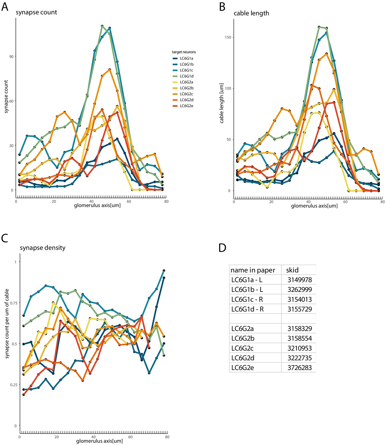
Quantification of the coverage of the glomerulus by the target neurons, using the same neuron color code and 1-μm-thick sections (but plotted for 20 equally spaced compartments) as in Figure 7—figure supplement 2: (A) synapse count, (B) cable length, and (C) the synapse density (the ratio of the synapse count per unit of cable in each section). (D) Table provides the names for each reconstructed target neuron as well as the ‘skid’ which is the numerical component of the Skeleton ID (used in CATMAID) that matches the labels for each skeleton (posted at https://fafb.catmaid.virtualflybrain.org/).
Figure 8 with 2 supplements
Interconnections between the LC6 glomeruli support contralateral suppression of visual responses to looming stimuli.
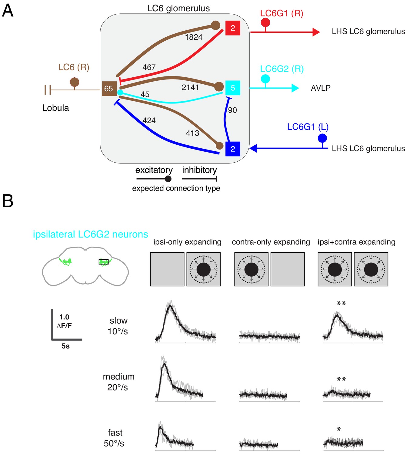
(A) A proposed microcircuit between LC6s, LC6G1, and LC6G2. Synapse counts are shown for observed connections in the EM reconstruction (above threshold of 15 synapses). Each colored box indicates one of the four groups of neurons in the connectivity matrix (Figure 7B), and the numbers of cells within each group are listed within each box. Based on expression of neurotransmitter markers (Figure 1—figure supplement 3), LC6 and LC6G2 are expected to be excitatory (indicated by the ball-shaped terminal), and LC6G1s are expected to be inhibitory (bar-shaped terminal). Within the glomerulus the line thickness indicates the number of synapses in each connection type (logarithmically weighted), which is also noted next to each connection. Outside of the glomerulus, arrowheads are used to depict the direction of the projection, away or towards the glomerulus. (B) Evoked calcium responses in LC6G2 by variations of bilateral looming stimuli. Looming stimuli are centered at ±45°. Responses for three different, constant speeds of looming. Mean responses from individual flies are in gray and mean responses across flies in black (N=4). The LC6G2 response is significantly reduced by the simultaneous presentation of a contralateral looming stimulus at all speeds (p = 2.2 × 10⁻³, p = 4.8 × 10⁻³, p = 2.3 × 10⁻² at 10, 20, 50°/s respectively, two-sided paired t-test). See Supplementary file 2 for summary of all looming visual stimuli presented.
Figure 8—figure supplement 1
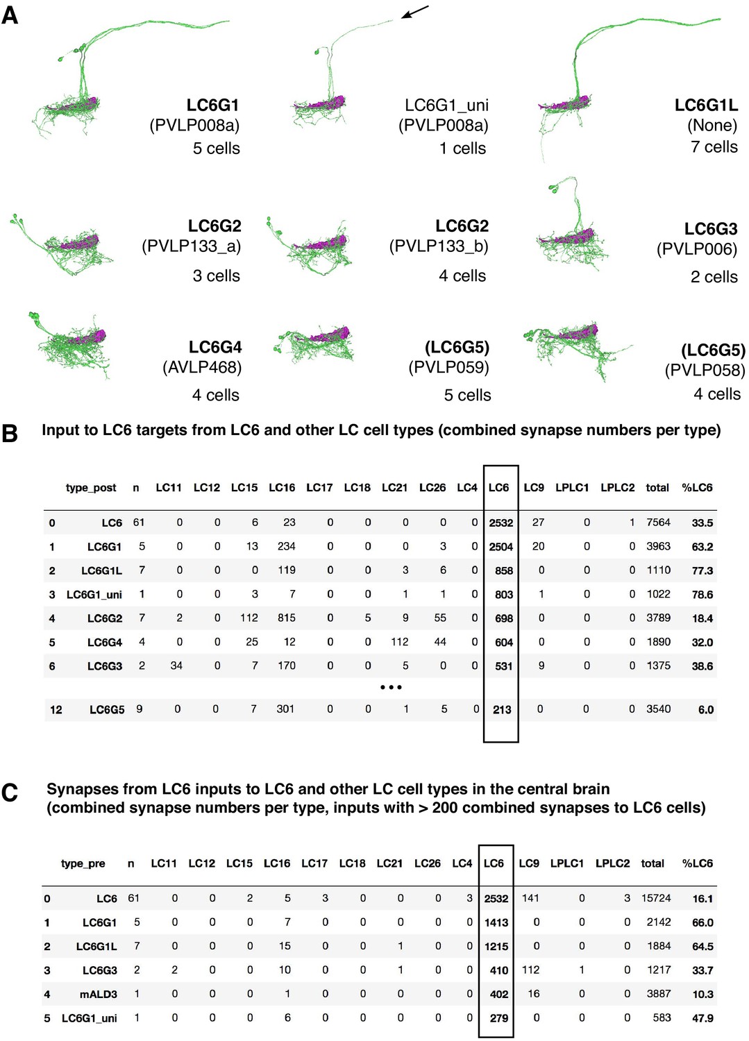
Hemibrain connectivity.
(A) LC6G cells in the hemibrain. Skeletons of LC6G candidates for each LC6G type are shown in groups. The approximate location of the LC6 glomerulus is indicated. Hemibrain release 1.1 cell typenames are in parenthesis. LC6G1_uni identifies a single reconstruction of a cell similar to LC6G1 that is either an incompletely reconstructed LC6G1 cell or a very similar cell without the projection to the contralateral glomerulus. (B) Main targets of LC6 cells in the hemibrain dataset and their input from LC6 and other selected LC cells. Synapse numbers are combined for the 61 reconstructed LC6 cells and for the cells of each named cell type. n indicates the number of cells per type for each row. LC6G1L refers to apparent contralateral LC6G1 projections (see A). Cell types are ordered based on the number of their combined synapses from LC6 cells. ‘%LC6’ indicates the proportion of the combined synaptic input of each cell type that comes from LC6 cells. Additional details on LC6G cells in the hemibrain and their connectivity can be found in Supplementary file 4. For details of how cell types were matched, see Materials and methods. (C) Main inputs to LC6 cells and selected other LC types. Details are as in (B). ‘%LC6’ is the proportion of a cell’s output synapses to LC6.
Figure 8—figure supplement 2
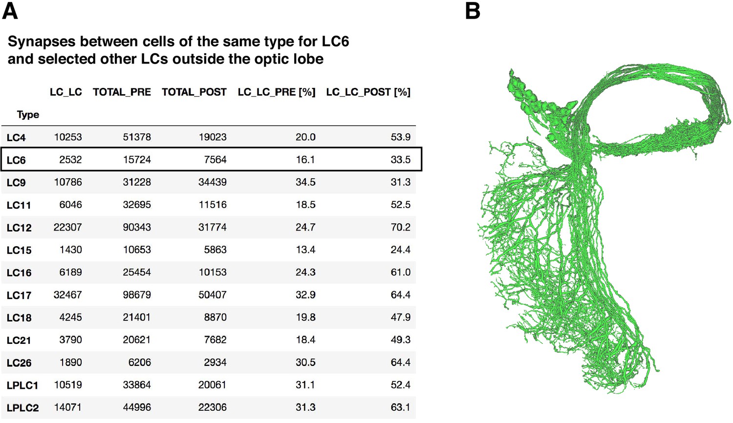
LC-LC synapses in the hemibrain dataset.
(A) Central brain synapses between LC cells of the same type in the hemibrain dataset. ‘LC_LC’ is the number of synapses between LC cells of the same type, ‘TOTAL_PRE’ and ‘TOTAL_POST’ indicate the total output and input synapses, ‘LC_LC_PRE’ and ‘LC_LC_POST’ the percentage of total outputs or inputs that are LC_LC synapses. LC types were identified using existing hemibrain annotations. (B) Morphology of the 61 named LC6 cells in hemibrain release 1.1.
Tables
Key resources table
| Reagent type (species) or resource | Designation | Source or reference | Identifiers | Additional information |
|---|---|---|---|---|
| Genetic reagent (Drosophila melanogaster) | OL0070B | https://doi.org/10.7554/eLife.21022.001 | OL0070B | LC6 split-GAL4 driver line available via https://www.janelia.org/split-GAL4. |
| Genetic reagent (D. melanogaster) | OL0081B | https://doi.org/10.7554/eLife.21022.001 | OL0081B | LC6 split-GAL4 driver line available via https://www.janelia.org/split-GAL4. |
| Genetic reagent (D. melanogaster) | SS00825 | This paper | SS00825 | LG6G1 split-GAL4 driver line, available via https://www.janelia.org/split-GAL4. |
| Genetic reagent (D. melanogaster) | SS00824 | This paper | SS00824 | LG6G1 split-GAL4 driver line, available via https://www.janelia.org/split-GAL4 |
| Genetic reagent (D. melanogaster) | SS02036 | This paper | SS02036 | LG6G2 split-GAL4 driver line, available via https://www.janelia.org/split-GAL4 |
| Genetic reagent (D. melanogaster) | SS02099 | This paper | SS02099 | LG6G3 split-GAL4 driver line, available via https://www.janelia.org/split-GAL4 |
| Genetic reagent (D. melanogaster) | SS02699 | This paper | SS02699 | LG6G3 split-GAL4 driver line, available via https://www.janelia.org/split-GAL4 |
| Genetic reagent (D. melanogaster) | SS03690 | This paper | SS03690 | LG6G4 split-GAL4 driver line, available via https://www.janelia.org/split-GAL4 |
| Genetic reagent (D. melanogaster) | SS02410 | This paper | SS02410 | LG6G5 split-GAL4 driver line, available via https://www.janelia.org/split-GAL4 |
| Genetic reagent (D. melanogaster) | SS02409 | This paper | SS02409 | LG6G5 split-GAL4 driver line, available via https://www.janelia.org/split-GAL4 |
| Genetic reagent (D. melanogaster) | SS25111 | This paper | SS25111 | LG6G5 split-GAL4 driver line, available via https://www.janelia.org/split-GAL4 |
| Genetic reagent (D. melanogaster) | SS03641 | This paper | SS03641 | LG26G1 split-GAL4 driver line, available via https://www.janelia.org/split-GAL4 |
| Genetic reagent (D. melanogaster) | pJFRC51-3XUAS-IVS-Syt::smHA in su(Hw)attP1, pJFRC225-5XUAS-IVS-myr::smFLAG in VK00005 | https://doi.org/10.1073/pnas.1506763112 | Presynaptic and membrane marker | |
| Genetic reagent (D. melanogaster) | MCFO-1: pBPhsFlp2::PEST in attP3;; pJFRC201-10XUAS-FRT > STOP > FRT-myr::smGFP-HA in VK0005, pJFRC240-10X-UAS-FRT>STOP > FRT-myr::smGFP-V5-THS-10XUAS-FRT > STOP > FRT-myr::smGFP-FLAG in su(Hw)attP1 | https://doi.org/10.1073/pnas.1506763112 | RRID:BDSC_64085 | MultiColor FlipOut (stochastic labeling) |
| Genetic reagent (D. melanogaster) | 42E06- LexA (JK22C) | https://doi.org/10.1534/genetics.114.173187 | ||
| Genetic reagent (D. melanogaster) | 13XLexAop2-CsChrimson-tdT (attP18), 20XUAS-IVS-Syn21-opGCaMP6f p10 (Su(Hw)attp8) | https://elifesciences.org/articles/49257/ and this paper | Functional connectivity | |
| Genetic reagent (D. melanogaster) | pJFRC7-20XUAS-IVS- GCaMP6m (VK00005) | 10.1038/s41592-019-0435-6 | RRID:BDSC_52869 | |
| Genetic reagent (D. melanogaster) | pJFRC48-13XLexAop2-IVS-myrtdTomato (su(Hw)attP8) | This paper | ||
| Genetic reagent (D. melanogaster) | UAS-7xHaloTag::CAAX (VK00005) | https://doi.org/10.1534/genetics.116.199281 | HaloTag reporter used for FISH | |
| Sequence-based reagent | FISH probes for GAD1, VGlut and ChaT | https://doi.org/10.1038/nmeth.4309 | ||
| Antibody | Anti-HA rabbit monoclonal C29F4 | Cell Signaling Technologies: 3724S | RRID:AB_1549585 | (1:300) |
| Antibody | Anti-FLAG rat monoclonal DYKDDDDK Epitope Tag Antibody [L5] | Novus Biologicals: NBP1-06712 | RRID:AB_1625981 | (1:200) |
| Antibody | DyLight 550 conjugated anti-V5 mouse monoclonal | AbD Serotec: MCA1360D550GA | RRID:AB_2687576 | (1:500) |
| Antibody | DyLight 549 conjugated anti-V5 mouse monoclonal | AbD Serotec: MCA1360D549GA | RRID:AB_10850329 | (1:500) |
| Antibody | Anti-Brp mouse monoclonal nc82 | DSHB | RRID:AB_2314866 | (1:30) |
| Software, algorithm | Python 3.7.8 | http://www.python.org | RRID:SCR_008394 | |
| Software, algorithm | neuprint python | https://github.com/connectome-neuprint/neuprint-python | ||
| Software, algorithm | FluoRender | http://www.sci.utah.edu/software/fluorender.html | RRID:SCR_014303 | |
| Software, algorithm | VVD_Viewer | https://github.com/takashi310/VVD_Viewer | ||
| Software, algorithm | Fiji | http://fiji.sc | RRID:SCR_002285 | |
| Software, algorithm | R | https://www.r-project.org/ | Anatomical analysis | |
| Software, algorithm | R studio | http://www.rstudio.com/ | ||
| Software, algorithm | Natverse package in R | http://natverse.org | EM anatomy tools | |
| Software, algorithm | MATLAB | Mathworks, Inc | Multiple versions 2016–2019 | Visual stimuli, experiment control, data analysis, and eye alignment |
| Software, algorithm | Nia (neuron image analysis) | https://bitbucket.org/jastrother/neuron_image_analysis | ||
| Software, algorithm | LED Panel display tools | https://github.com/reiserlab/Modular-LED-Display (Generation 3) | ||
| Software, algorithm | Thunder-project | https://github.com/thunder-project/thunder | http://thunder-project.org/ image registration – functional connectivity |
Additional files
-
Supplementary file 1
Detailed summary of genotypes used throughout the manuscript.
- https://cdn.elifesciences.org/articles/57685/elife-57685-supp1-v2.docx
-
Supplementary file 2
Detailed summary of visual stimuli.
- https://cdn.elifesciences.org/articles/57685/elife-57685-supp2-v2.docx
-
Supplementary file 3
Connectivity matrix of LC6 and target neurons from EM data.
- https://cdn.elifesciences.org/articles/57685/elife-57685-supp3-v2.pdf
-
Supplementary file 4
Hemibrain reconstructions of LC6G cell types and related cells (three tables).
Table 1. provides details of cells identified as likely matches of LC6G cell types in the hemibrain dataset as well as some related cells considered in the annotation process. The table includes the hemibrain identifiers (‘hemibrain_bodyId’), hemibrain cell type names (‘hemibrain_type’), LC6G annotations (‘new_type’), synaptic connections with LC6, LC16 and LC26 in the central brain and some notes related to the LC6G annotations. Table 2. lists all LC6 targets in the hemibrain (excluding other LC6 cells) that receive more than 100 combined central brain synapses from all LC6 neurons. Table 3. lists LC6 inputs in the hemibrain (excluding other LC6 cells) that provide more than 30 combined central brain synapses to all LC6 neurons.
- https://cdn.elifesciences.org/articles/57685/elife-57685-supp4-v2.xlsx
-
Transparent reporting form
- https://cdn.elifesciences.org/articles/57685/elife-57685-transrepform-v2.docx
Download links
A two-part list of links to download the article, or parts of the article, in various formats.
Downloads (link to download the article as PDF)
Open citations (links to open the citations from this article in various online reference manager services)
Cite this article (links to download the citations from this article in formats compatible with various reference manager tools)
Spatial readout of visual looming in the central brain of Drosophila
eLife 9:e57685.
https://doi.org/10.7554/eLife.57685


