Figures and data in Positive density dependence acting on mortality can help maintain species-rich communities | eLife

Figures
Additional files

7 figures and 3 additional files

Figures

Figure 1

Download asset Open asset

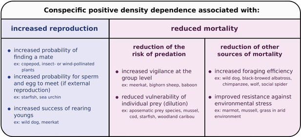
Mechanisms causing conspecific positive density dependence, and affecting reproduction or mortality.

For references and for a more exhaustive list, see the reviews by Courchamp et al., 1999; Stephens et al., 1999; Berec et al., 2007; Kramer et al., 2009. Note that two or more mechanisms causing positive or negative density dependence can occur simultaneously (Berec et al., 2007).

Figure 2

Download asset Open asset

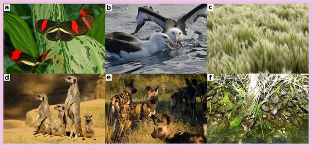
Example of organisms undergoing conspecific positive density dependence that associates with reduced mortality.

(a) Heliconius butterflies are aposematic (toxic and conspicuous) and therefore benefit from reduced predation when conspecifics are abundant. (b) Black-browed albatrosses in large flocks benefits from increased foraging efficiency and therefore from increased survival (Grünbaum and Veit, 2003). (c) Bottlebrush squirreltail in high density have a high survival rate and a high establishement success in arid grasslands (Sheley and James, 2014). (d) Meerkats in large group benefit from increased vigilance at the group level, reducing the risk of predation (Clutton-Brock et al., 1999). (e) Wild dogs in large group benefit from a high hunting success and defend effectively their kill against kleptoparasitism, thereby increasing their survival (Fanshawe and Fitzgibbon, 1993; Carbone et al., 1997). (f) Ribbed mussels in high density benefit from reduced crab predation and from improved winter ice resistance (Bertness and Grosholz, 1985). Photo credits: (a) Ettore Balocchi; (b) Ed Dunens; (c) Jeffry B. Mitton; (d) Ronnie Macdonald; (e) Barbara Evans; (f) Kerry Wixted.

Figure 3 with 3 supplements

Download asset Open asset

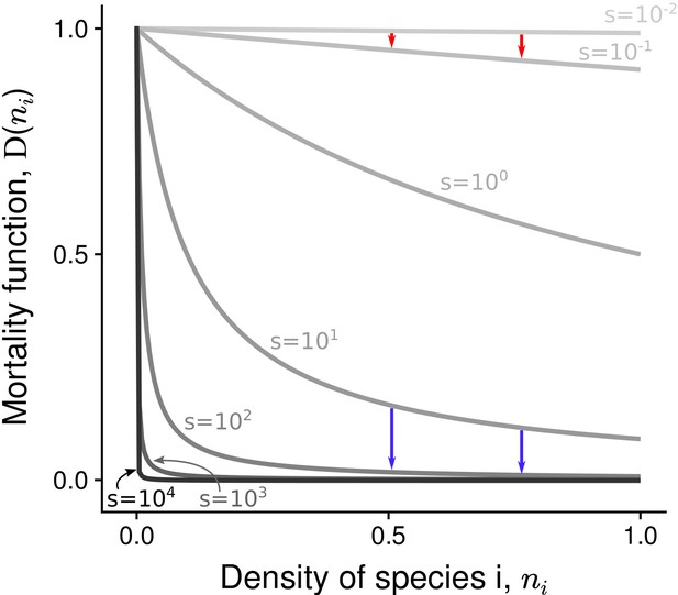
Non-linear mortality functions with different density-dependence factors ( $s$ ).

Pairs of arrows illustrate the non-linear effect of increased $s$ on mortality reduction. Depending on the value of the density-dependence factor $s$ , the most abundant species either benefits the most (red arrows) or the least (blue arrows) from increased $s$ .

Figure 3—figure supplement 1

Download asset Open asset

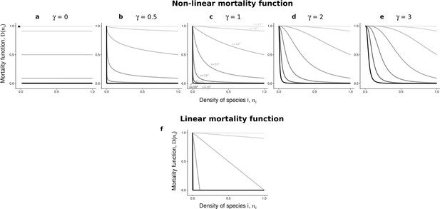
Non-linear and linear mortality functions with different density-dependence factors ( $s$ ) tested in supplementary analyses.

Non-linear and linear mortality functions with different density-dependence factors ( $s$ ) tested in supplementary analyses. In the case of non-linear mortality functions, $D (n_{i}) = \frac{1}{1 + s n_{i}^{γ}}$ is implemented (assuming $K = 1$ , otherwise the scaling shown in Supplementary file 1A is incorrect), and different values of exponent $γ$ making the curve sigmoidal are tested. For $γ = 0$ , $D (n_{i}) = 1$ if $n_{i} = 0$ , $D (n_{i}) = \frac{1}{1 + s}$ otherwise (i.e. increased $s$ associates with reduced mortality without density-dependence). In the case of linear mortality functions, $D (n_{i}) = \max [0, 1 - s n_{i}]$ is implemented.

Figure 3—figure supplement 2

Download asset Open asset

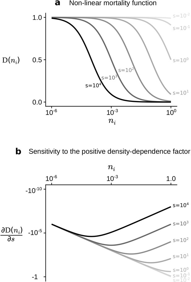
Sensitivity to increased density-dependence factor.

Non-linear mortality function (a) and its sensitivity to increased density-dependence factor (b) for different density-dependence factors ( $s$ ). Note the use of logarithmic scales. The partial derivative is $\frac{\partial D}{\partial s} = - \frac{n_{i}}{{(1 + s n_{i})}^{2}}$ , which is decreasing with $n_{i}$ if $n_{i} < 1 / s$ , and is increasing with $n_{i}$ if $n_{i} > 1 / s$ . Therefore, for increased density-dependence factor (increased $s$ ), species at high density do not necessarily incur a strong decrease in mortality ( $\frac{\partial D}{\partial s}$ is not always lower for higher $n_{i}$ ).

Figure 3—figure supplement 3

Download asset Open asset

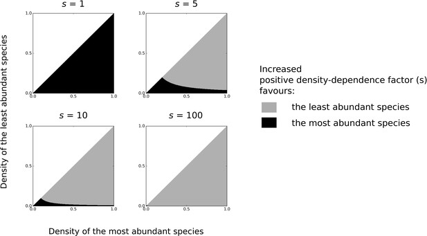
Effect of increased density-dependence factor on the mortality of the least vs. the most abundant species.

Effect of increased density-dependence factor on the mortality of the least vs. the most abundant species, determined from the values of $\frac{\partial D}{\partial s}$ for different values of $n_{i}$ (see Figure 3). For a high density-dependence factor (high $s$ ), the mortality rate of the least abundance species decreases the most with increased density-dependence factor (lower $\frac{\partial D}{\partial s}$ ).

Figure 4 with 4 supplements

Download asset Open asset

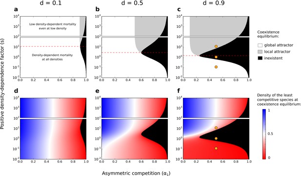
Effects of asymmetric competition for resources ( $α_{1}$ ) and positive density-dependence factor ( $s$ ) on coexistence.

Different values of the basal mortality rate ( $d$ ) are also tested. If the coexistence equilibrium exists, it is either a global attractor (it is reached independently of the initial conditions, as long as the two species start at density $> 0$ ) or a local attractor (it is not reached if the least competitive species is initially at a low density) (a–c). In each subfigure, the range of $s$ is arbitrarily divided in two; one range where there is conspecific positive density dependence at all densities, and another range where positive density-dependent mortality is very low even at very low densities (one might not consider those cases as conspecific positive density dependence). The dashed red lines correspond to the $s$ values above which increased density-dependence factor ( $s$ ) can favor coexistence (see Supplementary file 1B). Note the use of a logarithmic y-scale; the dashed red lines are not planes of symmetry. Orange dots corresponds to the combinations of parameters tested in Figure 5. Densities of the least competitive species at coexistence equilibrium are also represented (d–f). The growth rate of the most competitive species is not affected by the other species. Therefore, at the coexistence equilibrium, the density of the most competitive species correspond to the density of the least competitive species if $α_{1} = 0$ .

Figure 4—figure supplement 1

Download asset Open asset

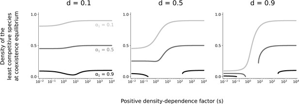
Densities at coexistence equilibrium.

Effects of asymmetric competition for resources ( $α_{1}$ ) and conspecific positive density dependence (depending on $s$ ) on densities at coexistence equilibrium, using analytical derivations. Different values of the basal mortality rate ( $d$ ) are also tested. If the coexistence equilibrium does not exist, the least competitive species always gets extinct (density $= 0$ , not shown here).

Figure 4—figure supplement 2

Download asset Open asset

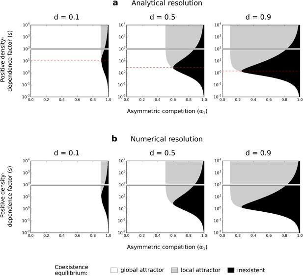
Identification of the coexistence equilibrium using analytical derivations or using the numerical resolution method.

Identification of the coexistence equilibrium in the model with asymmetric competition for resources, using analytical derivations (a) or using the numerical resolution method presented in Supplementary file 1C (b) (on system of Equations 1a and 1b). See Figure 4a-c and Figure 6 for more details.

Figure 4—figure supplement 3

Download asset Open asset

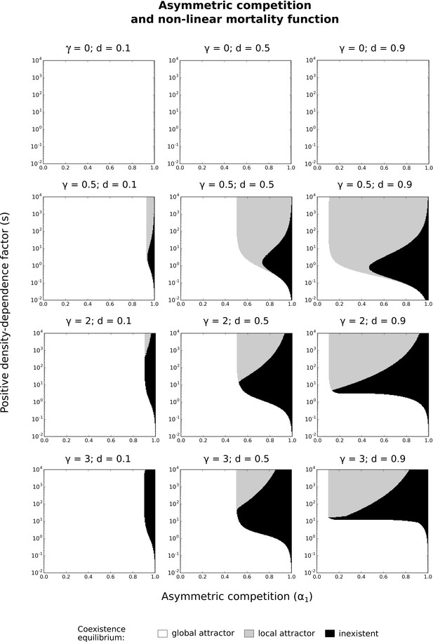
With other non-linear mortality functions.

Implications of other non-linear mortality functions for the effects of asymmetric competition for resources ( $α_{1}$ ) and positive density-dependence factor ( $s$ ) on coexistence. Different values of the basal mortality rate ( $d$ ) are tested. The numerical resolution method is used on the system of Equations 1a with the non-linear mortality functions $D (n_{i})$ described in Figure 3—figure supplement 1 (panels a-e; with different values of exponent $γ$ making the curve sigmoidal). See Figure 4 for more details.

Figure 4—figure supplement 4

Download asset Open asset

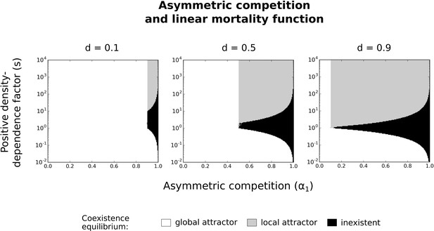
With a linear mortality function.

Implications of a linear mortality function for the effects of asymmetric competition for resources ( $α_{1}$ ) and positive density-dependence factor ( $s$ ) on coexistence. Different values of the basal mortality rate ( $d$ ) are tested. The numerical resolution method is used on the system of Equations 1a with the linear mortality functions $D (n_{i})$ described in Figure 3—figure supplement 1 (panel f). See Figure 4 for more details.

Figure 5

Download asset Open asset

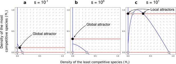
Effect of the positive density-dependence factor ( $s$ ) on the zero-net-growth isoclines in the case of asymmetric competition for resources.

Gray arrows represent the directions of the deterministic changes of species densities. Red and blue lines correspond to the isoclines (when $d n_{i} / d t = 0$ ) for species 1 and 2, respectively. Black and gray points represent stable and unstable equilibria, respectively. In each panel, the nature of the stable equilibria is annotated. Panel (a) corresponds to a case with a coexistence equilibrium that is a global attractor, panel (b) to a case without coexistence equilibrium, and panel (c) to a case with a coexistence equilibrium that is a local attractor. Other parameters: $d = 0.9$ and $α_{1} = 0.5$ , corresponding to the combinations of parameters represented by orange dots in Figure 4c and Figure 4f.

Figure 6 with 6 supplements

Download asset Open asset

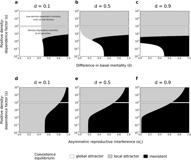
Effects of difference in basal mortality between species ( $δ$ ) (a,b,c) or asymmetric reproductive interference ( $α_{1}^{'}$ ) (d,e,f), and positive density-dependence factor ( $s$ ) on coexistence, using the numerical resolution method (systems of Equations 2 and 3, respectively).

If the coexistence equilibrium exists, it is either a global attractor or a local attractor. In each subfigure, the range of $s$ is arbitrarily divided in two; one range where there is conspecific positive density dependence at all densities, and another range where positive density-dependent mortality is very low even at very low densities. Because those two forms of species asymmetry do not promote species exclusion to the same extent, the levels of symmetric competition for resources are chosen as: $α = 0.5$ (a,b,c) or $α = 0$ (d,e,f).

Figure 6—figure supplement 1

Download asset Open asset

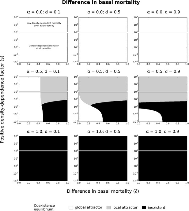
Difference in basal mortality with other levels of symmetric competition for resources.

Effects of difference in basal mortality between species ( $δ$ ) and positive density-dependence factor ( $s$ ) on coexistence, using the numerical resolution method (system of Equation 2). Different levels of symmetric competition for resources ( $α$ ) and basal mortality rates ( $d$ ) are tested. See Figure 6 for more details.

Figure 6—figure supplement 2

Download asset Open asset

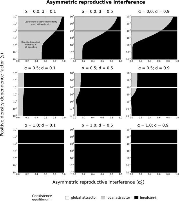
Asymmetric reproductive interference with other levels of symmetric competition for resources.

Effects of asymmetric reproductive interference ( $α_{1}^{'}$ ) and positive density-dependence factor ( $s$ ) on coexistence, using the numerical resolution method (system of Equation 3). Different levels of symmetric competition for resources ( $α$ ) and basal mortality rates ( $d$ ) are tested. See Figure 6 for more details.

Figure 6—figure supplement 3

Download asset Open asset

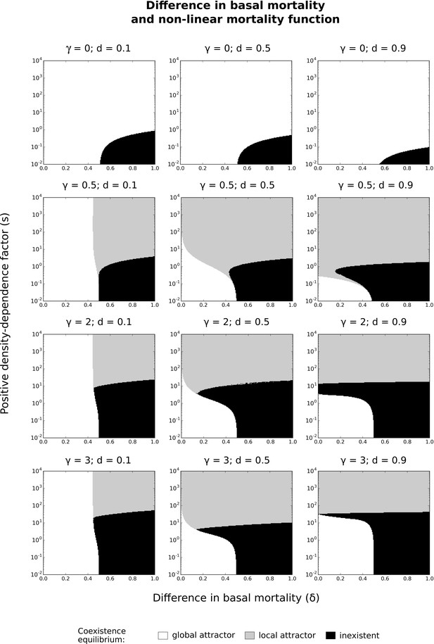
Difference in basal mortality with other non-linear mortality functions.

Implications of other non-linear mortality functions for the effects of difference in basal mortality between species ( $δ$ ) and positive density-dependence factor ( $s$ ) on coexistence. Different values of the basal mortality rate ( $d$ ) are tested. The numerical resolution method is used on the system of Equation 2 with the non-linear mortality functions $D (n_{i})$ described in Figure 3—figure supplement 1 (panels a-e; with different values of exponent $γ$ making the curve sigmoidal). Levels of symmetric competition for resources: $α = 0.05$ . See Figure 6 for more details.

Figure 6—figure supplement 4

Download asset Open asset

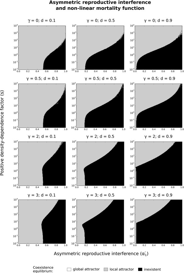
Asymmetric reproductive interference with other non-linear mortality functions.

Implications of other non-linear mortality functions for the effects of asymmetric reproductive interference ( $α_{1}^{'}$ ) and positive density-dependence factor ( $s$ ) on coexistence. Different values of the basal mortality rate ( $d$ ) are tested. The numerical resolution method is used on the system of Equation 3 with the non-linear mortality functions $D (n_{i})$ described in Figure 3—figure supplement 1 (panels a-e; with different values of exponent $γ$ making the curve sigmoidal). Levels of symmetric competition for resources: $α = 0$ . See Figure 6 for more details.

Figure 6—figure supplement 5

Download asset Open asset

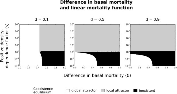
Difference in basal mortality with a linear mortality function.

Implications of a linear mortality function for the effects of difference in basal mortality between species ( $δ$ ) and positive density-dependence factor ( $s$ ) on coexistence. Different values of the basal mortality rate ( $d$ ) are tested. The numerical resolution method is used on the system of Equation 2 with the linear mortality functions $D (n_{i})$ described in Figure 3—figure supplement 1 (panel f). Levels of symmetric competition for resources: $α = 0.05$ . See Figure 6 for more details.

Figure 6—figure supplement 6

Download asset Open asset

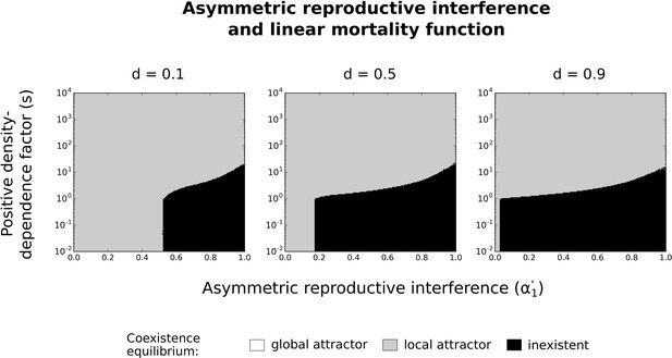
Asymmetric reproductive interference with a linear mortality function.

Implications of a linear mortality function for the effects of asymmetric reproductive interference ( $α_{1}^{'}$ ) and positive density-dependence factor ( $s$ ) on coexistence. Different values of the basal mortality rate ( $d$ ) are tested. The numerical resolution method is used on the system of Equation 3 with the linear mortality functions $D (n_{i})$ described in Figure 3—figure supplement 1 (panel f). Levels of symmetric competition for resources: $α = 0$ . See Figure 6 for more details.

Figure 7 with 9 supplements

Download asset Open asset

Species richness maintained in simulated communities.

Each box represents the distribution for 500 simulated communities with 100 species initially. (a) Only asymmetric competition for resources. (b) Only differences in basal mortality. (c) Only asymmetric reproductive interference. (d) Random communities with all forms of species asymmetry. In each subfigure, the range of $s$ is arbitrarily divided in two; one range where there is conspecific positive density dependence at all densities, and another range where positive density-dependent mortality is very low even at very low densities. Minimum basal mortality rate: $d = 0.5$ ; Levels of symmetric competition for resources: $α = 0.05$ (b) or $α = 0$ (c), competition for resources is asymmetric otherwise (a, d).

Figure 7—figure supplement 1

Download asset Open asset

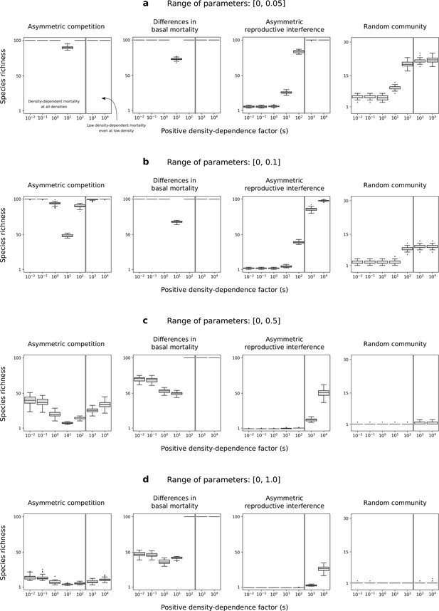
With parameters drawn from other uniform distributions.

Species richness in simulated communities when parameters are drawn from different uniform distributions. See Figure 7 for more details, and see full methods in Supplementary file 1D. Increasing the asymmetry among species decreases the overall remaining species richness, but does not change qualitatively the results regarding the effect of the positive density-dependence factor $s$ on species richness.

Figure 7—figure supplement 2

Download asset Open asset

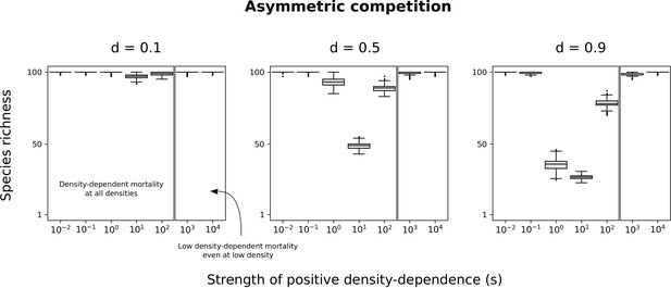
Asymmetric competition for resources with other minimum basal mortality rates.

Species richness maintained in simulated communities with only asymmetric competition for resources. Each box represents the distribution for 500 simulated communities. Different minimum basal mortality rates ( $d$ ) are tested. See Figure 7 for more details.

Figure 7—figure supplement 3

Download asset Open asset

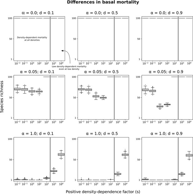
Differences in basal mortality with other minimum basal mortality rates and other levels of symmetric competition for resources.

Species richness maintained in simulated communities with only differences in basal mortality. Each box represents the distribution for 500 simulated communities. Different levels of symmetric competition for resources ( $α$ ) and minimum basal mortality rates ( $d$ ) are tested. See Figure 7 for more details.

Figure 7—figure supplement 4

Download asset Open asset

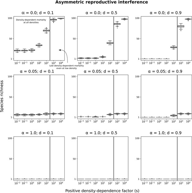
Asymmetric reproductive interference with other minimum basal mortality rates and other levels of symmetric competition for resources.

Species richness maintained in simulated communities with only asymmetric reproductive interference. Each box represents the distribution for 500 simulated communities. Different levels of symmetric competition for resources ( $α$ ) and minimum basal mortality rates ( $d$ ) are tested. See Figure 7 for more details.

Figure 7—figure supplement 5

Download asset Open asset

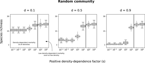
Random communities with other minimum basal mortality rates.

Species richness maintained in simulated communities with all forms of species asymmetry. Each box represents the distribution for 500 simulated communities. Different minimum basal mortality rates ( $d$ ) are tested. See Figure 7 for more details.

Figure 7—figure supplement 6

Download asset Open asset

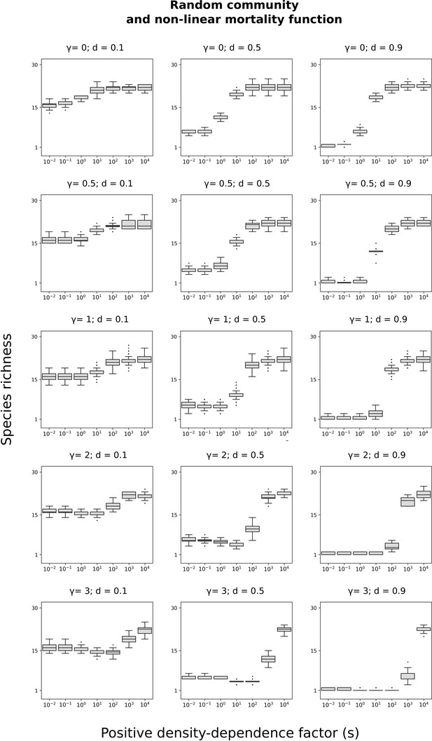
Random communities with other non-linear mortality functions.

Species richness in simulated communities with other non-linear mortality functions. Different minimum basal mortality rates ( $d$ ) are tested, and the non-linear mortality functions $D (n_{i})$ described in Figure 3—figure supplement 1 are implemented (panels a-e; with different values of exponent $γ$ making the curve sigmoidal). See Figure 7 for more details, and see full methods in Supplementary file 1D.

Figure 7—figure supplement 7

Download asset Open asset

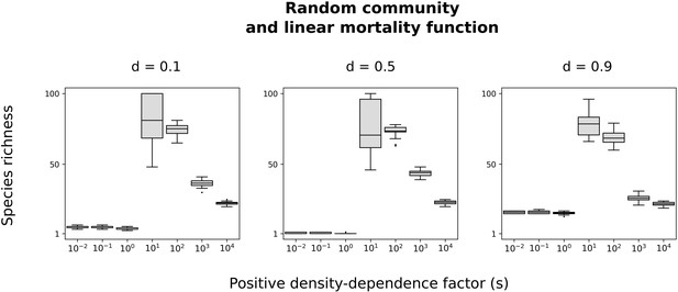
Random communities with a linear mortality function.

Species richness in simulated communities with a linear mortality function. Different minimum basal mortality rates ( $d$ ) are tested, and the linear mortality function $D (n_{i})$ described in Figure 3—figure supplement 1 (panel f) is implemented. Notably, species richness is high for intermediate $s$ values. See Figure 7 for more details, and see full methods in Supplementary file 1D.

Figure 7—figure supplement 8

Download asset Open asset

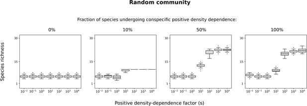
Random communities with only a fraction of species incuring conspecific positive density dependence.

Species richness in simulated communities when only a fraction of species incur conspecific positive density dependence. When a species does not incur conspecific positive density dependence, its density-independent mortality function is set to $D (n_{i}) = 1$ . Minimum basal mortality rate: $d = 0.5$ . See Figure 7 for more details, and see full methods in Supplementary file 1D.

Figure 7—figure supplement 9

Download asset Open asset

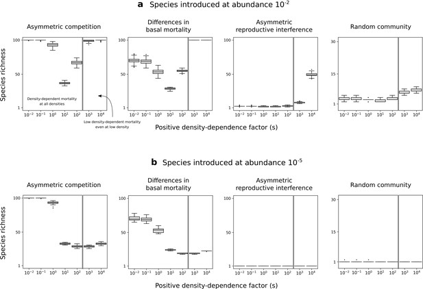
Random communities when species are introduced one at a time.

Species richness in simulated communities when species are introduced one at a time, either at abundance $= 10^{- 2}$ (a) or at abundance $= 10^{- 5}$ (b). Minimum basal mortality rate: $d = 0.5$ . See Figure 7 for more details, and see full methods in Supplementary file 1D. Species richness is lower because less competitive species (in the broad sense) may not invade the population. More importantly, conspecific positive density dependence does not help produce species-rich when species are introduced at low density (b).

Additional files

Supplementary file 1 Analytical derivations and supplementary information.: https://cdn.elifesciences.org/articles/57788/elife-57788-supp1-v1.pdf
Download elife-57788-supp1-v1.pdf
Source code 1 Simulation code.: https://cdn.elifesciences.org/articles/57788/elife-57788-code1-v1.zip
Download elife-57788-code1-v1.zip
Transparent reporting form: https://cdn.elifesciences.org/articles/57788/elife-57788-transrepform-v1.pdf
Download elife-57788-transrepform-v1.pdf

Download links

A two-part list of links to download the article, or parts of the article, in various formats.

Downloads (link to download the article as PDF)

Open citations (links to open the citations from this article in various online reference manager services)

Mendeley

Cite this article (links to download the citations from this article in formats compatible with various reference manager tools)

Thomas G Aubier

(2020)

Positive density dependence acting on mortality can help maintain species-rich communities

eLife 9:e57788.

https://doi.org/10.7554/eLife.57788

Sign up for email alerts

Privacy notice