Figures and data in Why is cyclic dominance so rare?

Figures
Tables
Additional files

15 figures, 8 tables and 1 additional file

Figures

Figure 1

Download asset Open asset

Cyclic dominance triplets across the scale of organisms.

In cyclic dominance, each type dominates one type and it is in turn dominated by another type. An arrow points from the dominated toward the dominant type. (A) The three actions in the game, Rock-Paper-Scissors cyclically dominate each other. (B) This game can also describe bacterial interactions (Kerr et al., 2002; Kirkup and Riley, 2004; Cascales et al., 2007): Some *E. coli* cells (orange) can produce a toxin that suppresses the survival of sensitive cells (blue). Hence toxin-producing cells (orange) dominate sensitive cells, whereas they are dominated by resistant cells (yellow). However in the absence of toxin-producing cells, the sensitive cells dominate resistant cells, exhibiting cyclic dominance. (C) Such dynamics can also occur in higher animals, as typified by the mating strategies of male side-blotched lizards (Sinervo and Lively, 1996; Sinervo et al., 2007): Strategies under which individual lizards guard many females (orange) can be invaded by a sneaker strategy that steals matings (yellow). If such a sneaker strategy is frequent, guarding a single mating partner (blue) can lead to higher mating success. However, once sneakers become rare again, guarding many females is beneficial, leading to cyclic dominance.

Figure 2

Download asset Open asset

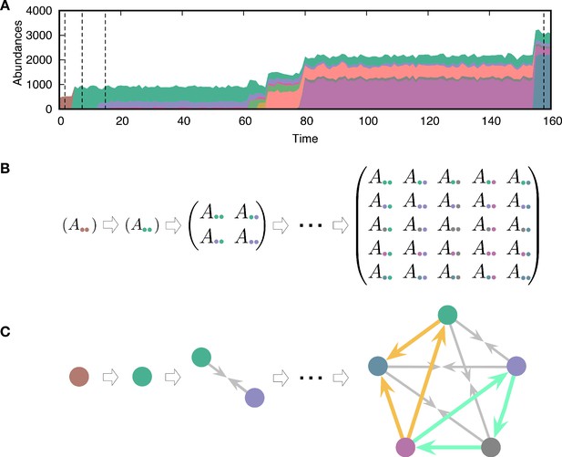
Evolving population dynamics and tracing its interactions and constructing a network.

(A) Sample simulation of population dynamics over time. Different colors correspond to different types. The colored area represents the abundance of each type. Time t is measured as the number of mutation events that occurred. (B) Interaction matrices between types at four different time points are marked by vertical dashed lines in panel A. Whenever a mutant emerges in the population, the diversity n increases and the payoff matrix becomes larger. Extinction of resident types can also happen because of the new mutant, reducing the size of the matrix. For example, one of the first mutant types (green) dominates the resident type (brown) and takes over the entire population. (C) Interaction structures inferred from the interaction matrices. There are three possible relationships: dominance (with two different directions indicated by an arrow from the dominated type to the dominant type), coexistence (arrows from each type to the middle), and bistability (arrows towards both types, not present here). We focused on triplets as basic substructures of the network. There are two triplets composed of three dominance links, but they have different topologies. One of them is cyclic dominance (highlighted in green), and the other is non-cyclic dominance (highlighted in yellow).

Figure 3

Download asset Open asset

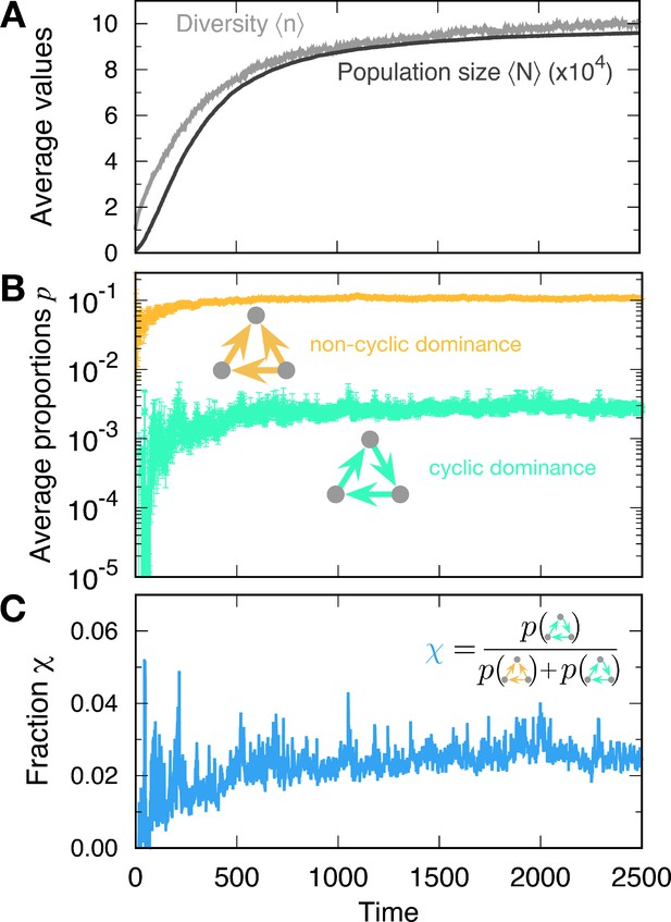
Formation of cyclic and non-cyclic dominance in the rapid mutation regime.

(A) For a low baseline death rate $α$ , the population size N tends to increases with new mutations. The average population size $⟨ N ⟩$ and diversity $⟨ n ⟩$ increase. When the population size N becomes large, cyclic and non-cyclic dominance can emerge. (B) Cyclic dominance triplets were less abundant than non-cyclic ones. In the long run, the proportions saturated at around 0.0036 and 0.105 for cyclic and non-cyclic dominance, respectively. (C) To quantify the rarity of cyclic dominance compared with non-cyclic dominance, we calculate the fraction $χ$ of cyclic dominance. In the early dynamics, it fluctuates because only a few realizations can form triplets because of the low average diversity. However, when large diversity is reached, the fraction became more stable, fluctuating around 0.033. This value is much smaller than the expected value when link types are randomly drawn ( $χ = 0.25$ ). indicating the rareness of cyclic dominance produced by novel mutations. (Simulation details: $λ_{b} = 0.9$ , $λ_{d} = 0.4$ , $α = 5 \cdot 10^{- 6}$ , $σ = 1$ , and $μ = 10^{- 5}$ . Unless we mentioned the parameter values, the same parameters were used for the following figures as well. The average is based on 4889 samples that did not go extinct among 5000 realizations. In each time point, the ensemble average in B and C is performed only for $n \geq 3$ at a given time.).

Figure 4

Download asset Open asset

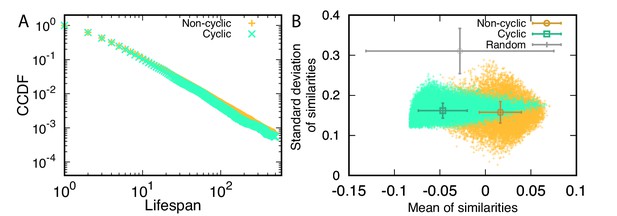
Properties of cyclic and non-cyclic dominance triplets.

(A) We traced the identified cyclic and non-cyclic dominance triplets and measured their lifespan in steady state, $9500 \leq t \leq 10000$ . The distributions of lifespan decayed algebraically, exhibiting a power law in the complementary cumulative distribution functions (CCDFs). The CCDF(x) shows the probability to have a lifespan longer than x. Both distributions were almost identical, but the tail component of non-cyclic dominance was slightly heavier. (B) We defined a trait vector of each type to characterize cyclic and non-cyclic dominances. A triplet consists of three vectors, and a set of scalar products can be calculated for all pairs. Scalar products are calculated after all payoffs are shifted and normalized so that the average payoffs becomes zero and the norms are one. A positive scalar product indicates that two types are similar. We used the mean and standard deviation of these similarities to characterize a triplet and draw a scatter plot. The symbols with error bars indicate the mean and standard deviation of quantities in each axis. For comparison, we performed the same calculation for random matrices. For both cyclic and non-cyclic triplets, the standard deviations of similarities are much smaller than that of random matrices. However the means of similarities for both triplets show different behavior. Types were less similar to each other in cyclic dominance compared to random matrices, while non-cyclic dominance has more similar types compared to random matrice. For this analysis, we used 1944 surviving realizations and $5 \cdot 10^{6}$ sets of random matrices.

Figure 5

Download asset Open asset

Genealogies and their effect on the fraction $χ$ of cyclic dominance.

(A). The scheme of genealogy. Vertical axis represents time, and horizontal axis represents mutational distance. Each solid vertical line corresponds to a single type. Horizontal lines indicate when mutation happens. Intermediary mutants can die out and a sequence of intermediary mutations is represented by a diagonal line. (B). An example of a genealogy for three types. Types i, j, and k are the types under consideration, and type o is their last common ancestor. Type n is the last common ancestor of j and k, and type m is the ancestor of the type i which existed at the moment when type j diverges from type k. Each of the three types has its own independent lineage from time $t_{d}$ on, and the fraction of accumulated mutations before and after this time determined the chance for cyclic dominance to emerge. For a list of all other possible genealogies, see Appendix 5. (C) For the sake of simplicity, we defined $F_{l}$ as the fraction of accumulated mutations after time $t_{d}$ compared to all mutations since the last common ancestor, $F_{l} = \frac{w_{2} + y + z}{w_{2} + y + z + w_{1} + x}$ . At the steady-state, when more mutations are accumulated after $t_{d}$ (large $F_{l}$ values), cyclic dominance can emerge more often by reducing the payoff correlations.

Figure 6

Download asset Open asset

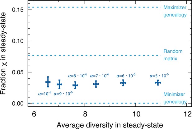
We compared the fractions $χ$ of cyclic dominance in the steady state for various baseline death rates $α$ from our simulations.

We also denoted three reference fractions: the maximizer genealogy ( $χ \approx 0.167$ ), random matrix ( $χ \approx 0.077$ ), and minimizer genealogy ( $χ$ <0.001). For various $α$ , the fractions of cyclic dominance were similar, although the average diversities in steady state were different. The majority of fractions $χ$ are between the one found for the minimizer geneaology and the fraction from the random payoff matrix. This implies that in the genealogies shaped by our population dynamics, the surviving offspring type is typically similar to the parental type. Each point is averaged over the surviving samples among 5000 realizations (4897, 4908, 4903, 4886, 4901, and 4889 samples for $α = 10^{- 5}, 9 \cdot 10^{- 6}, 8 \cdot 10^{- 6}, 7 \cdot 10^{- 6}, 6 \cdot 10^{- 6}, 5 \cdot 10^{- 6}$ , respectively).

Appendix 2—figure 1

Download asset Open asset

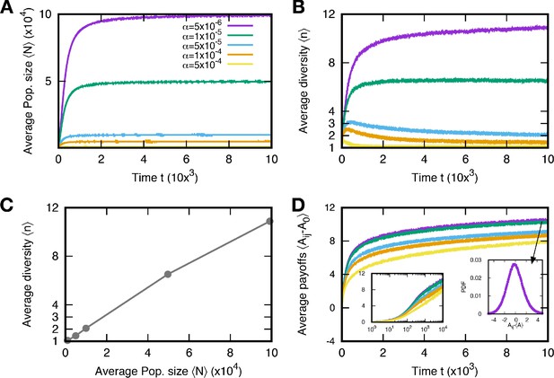
Population size and diversity for various baseline death rates $α$ .

The average population size $⟨ N ⟩$ and diversity $⟨ n ⟩$ in mutation event time t are shown in (A) and (B), respectively. We run 5000 independent simulations and use surviving samples at $t = 10000$ to obtain average quantities. The average population sizes and diversities at the stationary regime are determined by the baseline death rates: the larger the death rate, the smaller the population size and diversity. Also, both quantities have a positive correlation, see (C, D). As the populations evolve, the average payoffs $⟨ A_{i j} ⟩$ increase, but the increment decreases, indicating a weak selection regime. The initial payoff is denoted by A₀. Particularly, the average increases logarithmically in the stationary regime. The left inset is the same data as the main panel on a linear-log scale and shows the logarithmic increase of the average payoffs. The right inset is the probability distribution function of all payoffs in the steady state for $α = 5 \cdot 10^{- 6}$ . The distribution is smooth but slightly skewed to the left. ( $λ_{b} = 0.9$ , $λ_{d} = 0.4$ , $σ^{2} = 1$ , and $μ = 10^{- 5}$ ).

Appendix 3—figure 1

Download asset Open asset

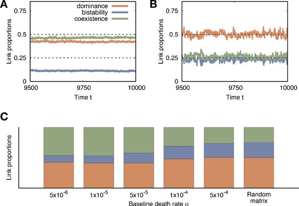
Average link proportions in the steady-state.

Time series of the average link proportions in the stationary regime for small baseline death rates (A, $α = 5 \cdot 10^{- 6}$ ) and large baseline death rates (B, $α = 5 \cdot 10^{- 4}$ ). The average runs over all surviving samples. C The average link proportions in the steady-state indicate different values for different $α$ . We averaged those values in time to get the representative link proportions in the stationary regime, $9500 \leq t \leq 10000$ . We find that large $α$ agrees with the values predicted by the random payoff matrix, because almost all links are formed by chance due to the low diversity. For small $α$ where the population size and the diversity are larger, we find more coexistence links, which tend to be stable for a long time.

Appendix 4—figure 1

Download asset Open asset

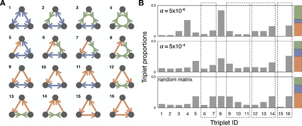
Triplet structures and their proportions.

(A) With three different link types, dominance with directionality, bistability, and coexistence, we can find 16 different triplet structures. We draw possible triplets and label them with an integer index we will refer to as Triad ID. (B) The average proportions of triplets in the steady-state are shown in the population dynamics with $α = 5 \cdot 10^{- 6}$ and $α = 5 \cdot 10^{- 4}$ and the random matrix. Since the link proportions strongly affect the triplet proportions, the direct comparison of triplets that have different link composition is meaningless. Thus, we focus on a set of triplets, which have the same link composition but a different structure. There are four such sets (6-7; 9-11; 12-14; 15-16), and we marked using dashed boxes for those sets in the panel. The last box indicates the cyclic and non-cyclic dominance triplets. For comparison, the colored stacked bar shows the proportions of the different link types for the corresponding value of $α$ .

Appendix 5—figure 1

Download asset Open asset

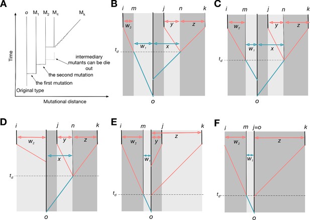
Possible genealogies for three types.

(A) The scheme of genealogy. Vertical axis represents time, and horizontal axis represents mutational distance. Each solid vertical line corresponds to a surviving type. Horizontal lines indicate when mutation happens. Intermediary mutants can be omitted and a sequence of intermediary mutations is represented by a diagonal line. (**B-E**) Four possible genealogies of three types. Types i, j, and k are focal types, and type o is their last common ancestor. Type n is the last common ancestor of j and k, and type m is the progenitor of type i existed at the moment when type j diverges from type k. The numbers of mutations between types are represented as $w_{1}, w_{2}, x, y$ , and z: $o \to m$ is w₁; $m \to i$ is w₂; $o \to n$ is x; $n \to j$ is y; $n \to k$ is z.

Appendix 5—figure 2

Download asset Open asset

Expression of payoffs derived from its parental payoffs Each element of payoff matrix in a triplet can be traced back to $A_{o o}$ .

However, due to the genealogy structure, some payoffs have additional common ancestors later than $A_{o o}$ . Note that for a genealogy at Appendix 5—figure 1D, $m = o$ and for Appendix 5—figure 1E, $n = o$ . Adding up the random variable $ξ$ to the payoff in the lower part gives the payoff in the upper part.

Appendix 6—figure 1

Download asset Open asset

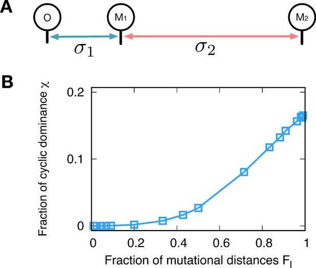
Minimal model.

(A) We can also shape the payoff correlation by controlling the sampling distribution. We use different variances of Gaussian noise for different mutation events, controlling the mutational distances. Mutational distances are controlled by not only how many steps proceed but also how big the jump is related variance of noise. Here, we assume a very simple genealogy type with different noise variances; The first mutant type M₁ originates from the type o with variance $σ_{1}^{2}$ while the second mutant M₂ mutated from M₁ has variance $σ_{2}^{2}$ for new payoffs. (B) Since only the relative mutational distances matter, we defined $F_{l} = \frac{σ_{2}}{σ_{1} + σ_{2}}$ . As we vary the fraction $F_{l}$ , we calculate the fraction $χ$ for three types o, M₁, and M₂. Small $F_{l}$ values give the same payoff structure of the minimizer while the maximizer is reproduced for large $F_{l}$ . The chance to observe the cyclic dominance triplets increases with $F_{l}$ , because types M₁ and M₂ become uncorrelated.

Appendix 7—figure 1

Download asset Open asset

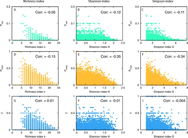
Scatter plots of diversity versus fractions of triplets.

In the first and the second rows, we plot $P_{c y c}$ and $P_{n c y c}$ for various diversities (in each column) in the steady-state. The last row shows the scatter plot for $χ = \frac{P_{c y c}}{P_{c y c} + P_{n c y c}}$ . For 1944 realizations, we measured the Pearson correlation coefficients and noted the correlation measured in each panel.

Appendix 7—figure 2

Download asset Open asset

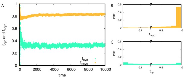
Average population frequencies belonging to cyclic and non-cyclic triplets $f_{c y c}$ and $f_{n c y c}$ over time.

(A) On average around 83% of population belongs to non-cyclic dominance triplets while only 33% population belongs to cyclic dominance triplets. (**B-C**) The probability distribution functions of $f_{n c y c}$ and $f_{c y c}$ are shown for each triplet. Non-cyclic dominance mainly emerges from majorities while cyclic dominance usually takes small population frequencies. Only 30% of the time, cyclic dominance can take over more than half of the population.

Author response image 1

Download asset Open asset

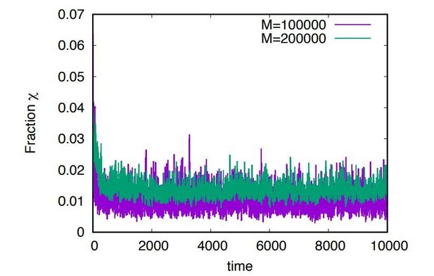
The average fraction \chi of cyclic dominance compared to non-cyclic dominance in time.

The payoffs are rescaled every mutation and extinction events so that the average of payoffs becomes zero. The population starts from a single-type population with the payoff zero. 2000 realizations are used for obtaining averages. At the steady-state, the average fractions are smaller than 0.02, which are smaller than that of our model.

Tables

Appendix 1—table 1

Given conditions, the stabilities of four fixed points are shown with its corresponding relationship between two types.

Stable fixed points are marked by S, while unstable fixed points are marke by U. Extinction is always unstable, while the stabilities of other fixed points depend on conditions. For the condition in the first row, $d_{11} < d_{21}$ and $d_{12} < d_{22}$ , type 1 can survive in the equilibrium, indicating the dominance of type 1. The second condition indicates the dominance of type 2. When both single-type fixed points are stable, the population can end up either type 1 or 2 population showing bistability. For the last condition, only the coexistence fixed point is stable.

Conditions	Fixed points				Relationship
Conditions	$(0, 0)$	$(x_{1}^{*}, 0)$	$(0, x_{2}^{*})$	$(x_{1}^{}, x_{2}^{})$	Relationship
$d_{11} < d_{21}$ and $d_{12} < d_{22}$	U	S	U	U	Dominance of type 1
$d_{11} > d_{21}$ and $d_{12} > d_{22}$	U	U	S	U	Dominance of type 2
$d_{11} < d_{21}$ and $d_{12} > d_{22}$	U	S	S	U	Bistability
$d_{11} > d_{21}$ and $d_{12} < d_{22}$	U	U	U	S	Coexistence

Appendix 4—table 1

Degeneracy of each triplet structure and their proportions in the random matrix.

Dashed boxes marks sets of triplets, which have the same link composition, but a different structure.

Triad ID	Degeneracy	Proportions
1	1	4/108
2	3	3/108
3	3	3/108
4	1	4/108
5	6	12/108
6	6	3/108
7	6	12/108
8	6	12/108
9	3	12/108
10	6	6/108
11	3	3/108
12	3	3/108
13	6	6/108
14	3	12/108
15	2	1/108
16	6	12/108

Appendix 6—table 1

Genealogies maximizing T₁₅.

Median values of each of five mutational distances $w_{1}, w_{2}, x, y, z$ are given. We use 12600 independent random initial values that each code one genealogy. We count how many of these genealogies belong to each class and sort classes by the average proportion of T₁₅.

Class	Counts	Proportion of T₁₅	w₁	w₂	X	Y	Z
$D^{15} - 1$	5044	0.020	0.0020	0.98	0	0	0.010
$D^{15} - 2$	2012	0.019	0	0	0	0	0.98
$D^{15} - 3$	683	0.016	0	0.0021	0.0017	0.37	0.59
$D^{15} - 4$	2701	0.014	0.0058	0.32	0	0.23	0.41
$D^{15} - 5$	2160	0.016	0.0046	0.52	0	0	0.44

Appendix 6—table 2

Genealogies minimizing T₁₆.

Median values of D_m are given. We use 20000 independent simulations.

Class	Counts	Proportion of T₁₆	w₁	w₂	X	Y	Z
$D_{16} - 1$	1576	0.11	0.0045	0.97	0	0	0.012
$D_{16} - 2$	697	0.11	0.0012	0.0021	0	0.011	0.96
$D_{16} - 3$	5883	0.11	0	0.29	0.019	0.22	0.45
$D_{16} - 4$	598	0.11	0.019	0.29	0.014	0.23	0.44
$D_{16} - 5$	11246	0.11	0.034	0.31	0	0.21	0.43

Appendix 6—table 3

Genealogies minimizing T₁₅.

Median values of D_m are given. We use 20000 independent simulations.

Class	Counts	Fraction of T₁₅	w₁	X	Y	Z
$D_{15} - 1$	4995	$< 10^{- 4}$	0.97	0.018	0	0.0051
$D_{15} - 2$	5011	$< 10^{- 4}$	0.014	0.97	0	0.0057
$D_{15} - 3$	9994	0.00012	0.48	0.49	0.0	0.014

Appendix 6—table 4

Genealogies maximizing T₁₆.

Median values of D_m are given.

Class	Counts	Proportion of T₁₆	w₁	X	Y	Z
D¹⁶-1	4772	0.24	0.97	0.025	0	0.0019
D¹⁶-2	11017	0.24	0.019	0.98	0	0.0023
D¹⁶-3	4211	0.24	0.45	0.53	0.0	0.0037

Appendix 6—table 5

Minimizer and Maximizer genealogies.

The fraction $χ$ of cyclic dominance is also calculated for each case.

Matrix generation	T₁₅	T₁₆
Random matrix	0.0093	0.11	0.077
Maximizer	0.02	0.11	0.154
Minimizer	< 10^-4	0.24	0.000

Appendix 7—table 1

Pearson correlation between diversity and fraction of cyclic and non-cyclic triplets.

In total 1944 realizations are used for the calculations and the average is across 500 time steps. We find a weak anti-correlation between the fraction of cyclic dominance and diversity while the fraction of non-cyclic dominance has stronger anti-correlation with diversity. Despite these differences, almost no correlation between the fraction and diversity is found.

	Richness index N	Shannon index H	Simpson index S
$P_{c y c}$	-0.05	-0.12	-0.11
$P_{n c y c}$	-0.15	-0.35	-0.34
$P_{c y c} f_{c y c}$	-0.04	-0.08	-0.07
$P_{n c y c} f_{n c y c}$	-0.12	-0.35	-0.34
	0.01	-0.01	-0.004

Additional files

Transparent reporting form: https://cdn.elifesciences.org/articles/57857/elife-57857-transrepform-v1.pdf
Download elife-57857-transrepform-v1.pdf

Download links

A two-part list of links to download the article, or parts of the article, in various formats.

Downloads (link to download the article as PDF)

Article PDF

Open citations (links to open the citations from this article in various online reference manager services)

Mendeley

Cite this article (links to download the citations from this article in formats compatible with various reference manager tools)

Hye Jin Park
Yuriy Pichugin
Arne Traulsen

(2020)

Why is cyclic dominance so rare?

eLife 9:e57857.

https://doi.org/10.7554/eLife.57857

Share this article

Cite this article

Cyclic dominance triplets across the scale of organisms.

Evolving population dynamics and tracing its interactions and constructing a network.

Formation of cyclic and non-cyclic dominance in the rapid mutation regime.

Properties of cyclic and non-cyclic dominance triplets.

Genealogies and their effect on the fraction χ of cyclic dominance.

We compared the fractions χ of cyclic dominance in the steady state for various baseline death rates α from our simulations.

Population size and diversity for various baseline death rates α.

Average link proportions in the steady-state.

Triplet structures and their proportions.

Possible genealogies for three types.

Expression of payoffs derived from its parental payoffs Each element of payoff matrix in a triplet can be traced back to Aoo.

Minimal model.

Scatter plots of diversity versus fractions of triplets.

Average population frequencies belonging to cyclic and non-cyclic triplets fcyc and fncyc over time.

The average fraction \chi of cyclic dominance compared to non-cyclic dominance in time.

Given conditions, the stabilities of four fixed points are shown with its corresponding relationship between two types.

Degeneracy of each triplet structure and their proportions in the random matrix.

Genealogies maximizing T15.

Genealogies minimizing T16.

Genealogies minimizing T15.

Genealogies maximizing T16.

Minimizer and Maximizer genealogies.

Pearson correlation between diversity and fraction of cyclic and non-cyclic triplets.

Transparent reporting form

Downloads (link to download the article as PDF)

Open citations (links to open the citations from this article in various online reference manager services)

Cite this article (links to download the citations from this article in formats compatible with various reference manager tools)

Genealogies and their effect on the fraction $χ$ of cyclic dominance.

We compared the fractions $χ$ of cyclic dominance in the steady state for various baseline death rates $α$ from our simulations.

Population size and diversity for various baseline death rates $α$ .

Expression of payoffs derived from its parental payoffs Each element of payoff matrix in a triplet can be traced back to $A_{o o}$ .

Average population frequencies belonging to cyclic and non-cyclic triplets $f_{c y c}$ and $f_{n c y c}$ over time.

Genealogies maximizing T₁₅.

Genealogies minimizing T₁₆.

Genealogies minimizing T₁₅.

Genealogies maximizing T₁₆.